Abstract
Temperature forecasting has been a consistent research topic owing to its significant effect on daily lives and various industries. However, it is an ever-challenging task because temperature is affected by various climate factors. Research on temperature forecasting has taken one of two directions: time-series analysis and machine learning algorithms. Recently, a large amount of high-frequent climate data have been well-stored and become available. In this study, we apply three types of neural networks, multilayer perceptron, recurrent, and convolutional, to daily average, minimum, and maximum temperature forecasting with higher-frequency input features than researchers used in previous studies. Applying these neural networks to the observed data from three locations with different climate characteristics, we show that prediction performance with highly frequent hourly input data is better than forecasting performance with less-frequent daily inputs. We observe that a convolutional neural network, which has been mostly employed for processing satellite images rather than numeric weather data for temperature forecasting, outperforms the other models. In addition, we combine state of the art weather forecasting techniques with the convolutional neural network and evaluate their effects on the temperature forecasting performances.
1. Introduction
Weather forecasting is one of the most steadily researched areas because the weather has a significant impact on humans’ daily lives as well as various industry sectors [1,2,3]. Among weather factors, temperature is considered the most important because it is closely related to energy generation and agricultural operations [4,5,6,7]. In particular, minimum and maximum temperatures can have adverse impacts on agricultural operations in extreme events, so accurate temperature forecasting plays an important role in preventing agricultural damage [8]. However, weather factors including temperature are continuous, data-intensive, multidimensional, dynamic, and chaotic, and thus, it is ever-challenging to accurately predict temperature [9].
Researches on weather forecasting are mainly performed in two ways, physics-based and data-driven models. First, physics-based weather forecasting models directly simulate physical processes that numerically analyze the effects of atmospheric dynamics, heat radiation, and impact of green space, lakes, and oceans. Most commercial and public weather forecasting systems still consist of physics-based models [10,11,12]. On the other hand, data-driven models perform weather forecasting using statistics or machine learning-based algorithms. The data-driven models have the advantage of being able to identify unexpected patterns for the meteorological system without any prior knowledge. However, it can require a large amount of data, and there is a lack of interpretation of how the models work. Contrary, the physics-based methods have the advantage of being interpretable and having the potential for extrapolating over observed conditions. However, it has the disadvantage of requiring well-defined prior knowledge and a large computational capacity [13,14]. Recently, data-driven models for weather forecasting have been more actively studied with the increase in the number of available features and observations.
To overcome these challenges, research has increased steadily on temperature forecasting, in two main directions. One is that researchers have used time-series analysis based on autoregressive integrated moving average (ARIMA) to study longer-term predictions such as monthly and annual [15,16,17]. The other is machine learning algorithms based on neural network models for shorter-term predictions such as hourly and daily.
Existing research has mostly been focused on forecasting temperatures using consistent time unit data. Specifically, both the input data and the target data are the same time unit, for example, using daily input data to forecast day-ahead temperature. However, as the amount of available high-frequent data has increased and computing power using graphics processing units has improved, it is possible to use hourly input data for daily temperature forecasting, as opposed to only the daily input data that could previously be used. Both hourly and daily patterns can be employed to forecast daily temperatures, but because these data are abundant and detailed, it is essential to process them efficiently and effectively. In this context, neural network models have powerful versatility to process large amounts of more detailed data.
In this study, we forecast daily average, minimum, and maximum temperatures with different time-interval data using deep neural network models. Our major contributions are as follows. First, unlike in previous studies, we used detailed time unit input data rather than target data to forecast day-ahead temperature. Second, to enable efficient and effective processing of more detailed and abundant data, we used three neural network models: multilayer perceptron (MLP), long-short term memory (LSTM), and convolution neural network (CNN). In particular, we applied a CNN, which has been mostly employed for satellite data in previous studies, to numeric weather data with a suitable structure for them, and we, in fact, found that it outperformed the other models. Third, we compared the models for factors such as time unit of input data, time length of input data, regions, and neural network models. In addition, we combined the recent state of the art techniques in weather forecasting such as multimodal learning and multitask learning and examined their effects on temperature forecasting performance. For multimodal learning, we performed temperature forecasting by employing additional satellite images as well as the existing numerical meteorological data. For multitask learning, we predicted several temperatures simultaneously to take advantage of shared information among different types of temperatures in different regions. To analyze the effectiveness of multimodal learning and multitask learning, we compared their results with those of the ordinary models.
The rest of the paper is organized as follows. In Section 2, we present the literature review. In Section 3, we introduce the neural network architectures we proposed for forecasting the temperature. In Section 4, we describe the data we used and how to preprocess the data. Section 5 presents the experimental design and our interpretation of the results. In Section 6, we conclude the paper with a summary.
2. Related Work
2.1. Data-Driven Temperature Forecasting
Researchers have performed data-driven temperature forecasting for a few decades, and there are two main research directions: time-series analysis based on ARIMA and machine learning algorithms based on neural network models. For the former, ARIMA is a linear statistical technique for analyzing and forecasting time series. The key components of the model are auto-regressive, integrated, and moving average. Briefly, the integration component makes data stationary through differentiating, and the auto-regressive component uses the dependency between some number of lagged data and the moving-average accounts for previous error terms. For the latter temperature prediction research direction, neural network models have been the most actively studied of the machine learning algorithms for forecasting time series. Neural network models have strong power to solve many kinds of nonlinear problems and can capture the relationships between input and target data. Furthermore, they are applicable even when the units of data are different, whereas traditional methods require the same units of data.
Researchers have mainly studied ARIMA models for forecasting temperatures for longer time units, such as monthly and annual. For instance, one ARIMA model was used to forecast monthly temperatures for Assam in India, specifically the variant of ARIMA called seasonal autoregressive integrated moving average to reflect the seasonality [15]. In another study, an ARIMA model was used to analyze annual rainfall and maximum temperature and forecast for watershed and agricultural management [17]. Researchers also used the variant of ARIMA known as autoregressive fractionally integrated moving average to forecast monthly temperature and precipitation time series [16].
Meanwhile, researchers have used neural networks to forecast temperatures for shorter time units such as hourly and daily, including to forecast hourly temperature for load forecasting; these authors first forecast daily temperatures to predict daily temperature trends and used these to forecast hourly temperatures [18]. In another study, researchers developed an ensemble of neural network models to forecast various weather factors such as hourly temperature wind speed, and relative humidity [9], and others combined ARIMA and neural network models to forecast hourly temperatures [4]. These authors first used ARIMA to forecast temperatures and used the forecast values as inputs in the neural network for stable and accurate forecasts.
Most researchers to date have used the same time units for both input and target data, but neural network models are versatile and can accommodate different input and target data units. Therefore, it is possible to employ more specific input data than target data for better forecasting performance. Better forecasting requires the capacity to process abundant and specific data efficiently and effectively with proper neural network model architectures.
2.2. Neural Networks for Signal Processing
Forecasting temperatures using numeric weather data with different time units can be viewed as signal processing because numeric weather data have sequences over time, and applications of signal processing using neural network models have used different types of input and target data. The main application areas of signal processing are speech recognition and bio-signal recognition, as well as time series forecasting [18,19,20,21,22,23,24,25,26,27]. Researchers have used two typical neural network models for signal processing: recurrent neural networks (RNNs) and CNNs.
RNNs are specialized for sequential data such as signal, time series, and text. These networks have a component called hidden state that is a function of all previous hidden states and that allows RNNs to perform well with sequential data. However, RNNs have a critical limitation, a vanishing gradient problem. The LSTM model is an advanced RNN; it includes the gates in RNN, and it addresses the vanishing gradient problem, allowing the model to perform much better than RNNs [28]. In the signal processing research with LSTM, [22] performed speech recognition tasks using deep LSTM, and that model outperformed those used in previous studies. Deep LSTM reflects the long term effectively through multiple levels of representation. In one study, [24] predicted seizures using LSTM to process electroencephalogram signal data. In another study, [27] used deep bidirectional LSTM network-based wavelet sequences to classify electrocardiogram signals, and their model showed better recognition performance than that of conventional networks.
Researchers have used CNNs with success in computer vision, and they have performed well with speech recognition as well. CNNs have the key aspects of sparse interaction and parameter sharing using convolution layers with considerably fewer parameters than with MLP [29]. In research on signal processing using CNN, [21] performed speech recognition using CNN models, and their models outperformed the MLP models and hidden Markov model that had been used in previous studies. [19] used a CNN to process electrocardiogram data to predict various cardiovascular diseases, and others [23] used a CNN to process electroencephalogram signal data and diagnose epilepsy. In both of these studies, the researchers used CNNs with one-dimensional signal data; however, in a different study, [30] used two-dimensional electroencephalogram signal data, which enabled brain-computer interaction.
Researchers have recently been studying both LSTM and CNNs to forecast time-series data. [7] used LSTM combining ensemble empirical mode decomposition and fuzzy entropy to forecast wind speed. [31] conducted and analyzed stable forecasting of environmental time series using LSTM or [3] employed CNN to process one-dimensional signal data to forecast monthly rainfall; in the latter study, the authors represented input data in one-dimensional signals using various weather factors. However, this method does not consider that the order of weather variables is independent. Furthermore, the methods mentioned above-employed input data and target data with the same time units. Most existing studies on temperature-related tasks using CNNs have been employed satellite data. [32] forecasted sea surface temperature field by processing satellite data with the combination of CNN and LSTM and [33] predicted subsurface temperatures by using CNN with satellite remote sensing data. In this study, we performed air temperature forecasting by applying the CNN to numeric weather data rather than satellite data with a suitable structure to process them.
Most recently, various machine learning approaches, including multimodal learning which combines different types of inputs to perform specific tasks and multitask learning which learns related tasks simultaneously for computational efficiency and performance improvement by using shared information among related tasks, have been applied to the weather forecasting. [34] performed solar irradiance prediction by employing both numerical meteorological data and the images of sky. [35] predicted rainfall at multiple sites simultaneously with multitask learning and [36] forecasted wind power ramp events using multitask deep neural networks.
3. Proposed Neural Network Architectures
We used three neural network structures, MLP, LSTM, and CNN, with two different types of time unit input data, daily and hourly, to forecast daily temperatures. We built the six models by pairing each structure with each time unit as follows:
- MLP with daily input variables
- MLP with hourly input variables
- LSTM with daily input variables
- LSTM with hourly input variables
- CNN with daily input variables
- CNN with hourly input variables
The detailed structures of each model are explained in Table 1, Table 2, Table 3, Table 4, Table 5 and Table 6 and Figure 1 and Figure 2. Note that T and m shown in Table 1, Table 2, Table 3, Table 4, Table 5 and Table 6 denote the length of time of the input data and the number of input variables, respectively.

Table 1.
The architecture of multilayer perceptron (MLP) with daily input data.
Table 2.
The architecture of MLP with hourly input data.
Table 3.
The architecture of LSTM with daily input data.
Table 4.
The architecture of LSTM with hourly input data.
Table 5.
The architecture of CNN with daily input data.
Table 6.
The architecture of CNN with hourly input data.
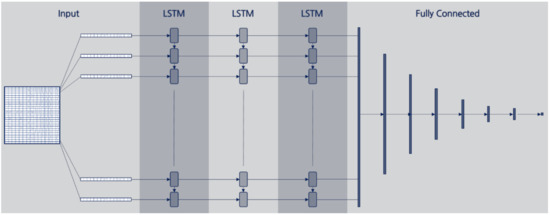
Figure 1.
Model structure of long-short term memory (LSTM) for temperature forecasting.
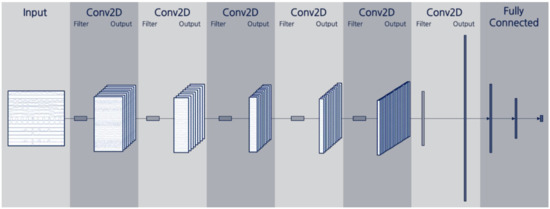
Figure 2.
Model structure of convolution neural network (CNN) for temperature forecasting.
3.1. MLP
MLP is one of the most common neural network model structures for regression and classification, which propagates information layers by layers. MLP consists of layers containing more than one perceptron with activation functions and their connections; it receives input data by the input layer, and these data are transmitted throughout the hidden layers and the output layer through connections. Then, the output layers return the predicted values. One of the typical ways for calculating an output value for each node is as follows:
where is the output value of each node, is the input from connected node in the previous layer, ’s are learnable weight parameters, and is an activation function. Typically, hyperbolic tangent function, logistic function, and rectified linear units are selected for activation functions.
Table 1 and Table 2 represents the architectures of the MLP models in this study using the daily and hourly input data, respectively; we determined these through trial and error. T and m in Table 1 and Table 2 denote time length of input data and the number of input variables. For example, with three days of input data in MLP with daily input data, the number of input nodes is 51: 3 (days) × 17 (variables). Likewise, with three days of input data in MLP with hourly input data, the number of input nodes is 1080: 3 (days) × 24 (h) × 15 (variables).
3.2. LSTM
The LSTM model is an advanced RNN model that reflects temporal dependencies between input data better than RNN by introducing the gates for controlling temporal information to the hidden state. The LSTM model has dealt with a vanishing gradient problem of the RNN model and is one of the most powerful artificial neural network models for sequential data such as text, signal, and time series. The LSTM model consists of connections of cells which contains a hidden layer and an output layer. A hidden layer receives an input and a context , values of the hidden layer of the previous cell, as inputs and then derives a hidden context vector from the inputs and an output layer calculates output vector with the hidden context vector as the following equations:
where the gate vectors and cell state vectors , , , , and weight matrices and bias vectors , , , , , are learnable parameters, and denotes a sigmoid function. After deriving the LSTM cell returns the output vector by combining it with and in the output layer.
We designed the LSTM structures in this study as three stacked LSTMs connected to the fully connected layer. We describe LSTM model architectures in Figure 1, and Table 3 and Table 4 summarize the details of the daily input and hourly input LSTM model structures, respectively. If the number of input variables is 17, the first cell receives a 17-dimensional vector as an input and extends it to a 20-dimensional vector before it passes to the second cell. In the case of hourly input data, however, the LSTM model keeps the number of vector dimensions as the number of input variables m. As we noted earlier, we determined the remaining structure of the LSTM model through trial and error. Note that T and m shown in Table 3 and Table 4 denote the length of time of the input data and the number of input variables, respectively.
3.3. CNNs
CNNs have the key aspects of sparse interaction and parameter sharing using convolution layers with considerably fewer parameters. CNNs consist of three major components: convolution, pooling, and fully connected layers. In convolution layers, the convolution operation is performed to extract the local features. The convolution operation for two-dimensional case, for example, is as follows:
where is a matrix containing the input values, is a convolution filter matrix sliding across the input, and denote row and column indices in the input, and is output value at a location , respectively. The pooling layer reduces the dimension of output neurons with pooling operation, or down-sampling, which reduces several values into one. The most common pooling operations are max-pooling, average-pooling, and min-pooling, which derive maximum, average, and minimum value in a group, respectively. The fully connected layer is the same with MLP, taking inputs from the previous layer, processing them with activation functions, and transmitting them to the next layer.
In this study, to apply a CNN to the multivariate climate input data, we represented the input data on one axis for the time sequence and the other axis for each variable. For example, if three days of hourly input data is used, the length of the axis for time is 72, and the other axis is 15 for each variable, for a 72 × 15 rectangular input channel.
Because one axis of the input channel is composed of variables and the order of these variables is independent, we designed one axis of all convolution filters except for the last convolution layer with a length of 1 in order not to cross process each variable. After it passes all the convolution layers except for the last one, the convolution channel will have a time axis length of 1 and a variable axis length equal to the number of variables. Then, we designed the convolution filters of the last convolutional layer to have the same structure as the output channel of the previous layer and for the convolution filters to give a single value as output, respectively. Subsequently, the output consists of as many values as the number of filters, and they are connected to the fully connected layers to forecast temperatures.
4. Data
In this section, we introduce the numeric weather data we used and describe the data preprocessing. After preprocessing, we generated data in different time units; we collected the data as hourly units, and we generated additional daily data from the hourly data by taking daily averages for each variable. In addition, we generated daily minimum and maximum temperatures, and we used the generated data as both input and target data.
4.1. Data Description
We collected the numeric weather data observed from the Automated Surface Observing System operated by the Korea Meteorological Administration [37]. The Automated Surface Observing System (ASOS) is a manned weather measurement system where the Korea Meteorological Administration maintains and observes weather elements. We selected three ASOS stations in South Korea as shown in Figure 3, representing metropolitan, Seoul; mountainous, Daegwalleong; and coastal, Seongsan. There are 96 ASOS stations in operation in South Korea, and the average, maximum, and minimum distances from one center to its nearest center are 32.6 km, 142.3 km, and 13.7 km, respectively [38,39]. Note that the proposed deep neural network models perform pointwise temperature forecasting at the ASOS station where the target variable is collected. We stated whether the input data from the stations other than that corresponding to the target variable were used or not, for each experiment in this study, in Section 5.1. We collected 10-year data, from 2009 to 2018, in hourly time units, and we used 15 input variables: temperature, amount of water precipitation, humidity, vapor pressure, dew point temperature, atmospheric pressure, sea-level pressure, hours of sunshine, solar radiation quantity, amount of snowfall, total cloud cover, middle- and low-level cloud cover, ground-surface temperature, wind speed, and wind direction. The meteorological measurement methods of each variable are as follows [40]: (1) all temperatures are measured in every minute with an average of the last five minutes. (2) all pressure variables are measured by several pressure sensors and recorded every minute and compared with standard references for accurate measurements. (3) amount of water precipitation is recorded every minute based on observing accumulated amount of amount of water precipitation using cylinder and applying a post-processing algorithm. (4) humidity is calculated using the five-minute averaged temperature and dew point temperature. (5) hours of sunshine are observed by a sunshine sensor and recorded the cumulative time of sunlight in every minute. (6) solar radiation is observed using a pyranometer and recorded in every minute. (7) amount of snowfall is recorded in every minute by using the cylinder with heating system. (8) total, middle-level, and low-level cloud cover rely on human observation and are recorded in deciles in every hour. (9) wind direction and speed are recorded every minute using the past two-minute average of five-second averaged values. After collecting the data, in this study, we converted all observed variables to hourly unit by selecting the records on the hour.
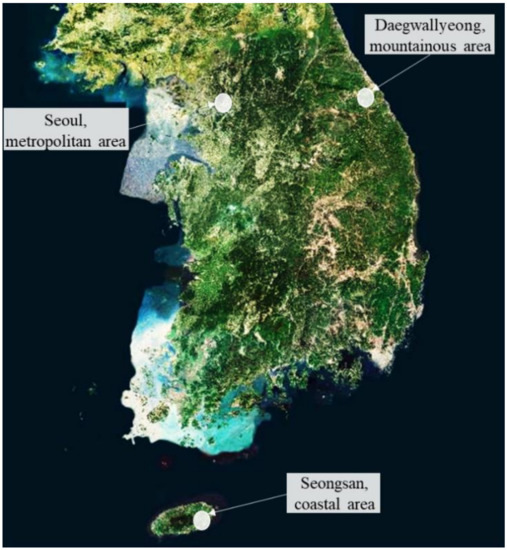
Figure 3.
Selected regions in South Korea. Map is from Korea National Geographic Information Institute [41].
4.2. Data Preprocessing
For the data preprocessing, we first replaced the missing values from the data and then converted the wind direction and speed to x-component and y-component.
4.2.1. Missing Values
Missing values in this study can be classified into two cases: Missing values can occur intentionally during data collection or by accident such as through mistakes or machine defects. The former occurs regularly, so there are many missing values, but the latter errors are rare. Therefore, we treated the two types of missing values differently.
First, intentional missing values were left blank on purpose. For instance, Table 7 shows the number of missing values for solar radiation, and these data points were left blank because the time units occurred during the evening and at dawn when the sun was not up; as such, we could replace these missing values with 0. Amount of water precipitation, amount of sunshine, amount of snowfall, total cloud cover, and middle-and low-level cloud cover were also deliberately missed, and thus we processed these variables in the same way.
Table 7.
Missing values for solar radiation.
Second, there were few missing values for data that are measured 24 h per day, such as temperature and humidity. In these cases, because there were few missing values, we replaced them with the values one time step before. For example, if a missing value occurred at 13:00 on 8 August 2009, we replaced it with the value at 12:00 on 8 August 2009.
4.2.2. Wind Direction and Wind Speed
The wind direction is recorded as 1 degree and 359 degrees, which are in fact very close, but it is recognized that the difference is 358 degrees when they are expressed numerically. Therefore, we converted the wind direction with the wind speed into x-component and y-component as in (9) and (10), as expressed in [42].
where V is wind speed and θ is wind direction.
4.3. Basic Statistics
After data preprocessing, we generated additional daily data using the hourly data. We used the daily data as target data for temperature forecasting tasks using three types of daily temperatures and as another input data for comparison. We introduce the hourly and daily data as follows.
4.3.1. Hourly Data
Table 8, Table 9 and Table 10 show the basic statistics for the hourly unit data for the three selected regions; these basic statistics show clear differences between the three regions. In particular, the temperature, amount of water precipitation, and atmospheric pressure in Seongsan and Daegwallyeong clearly show such regional characteristics. We note here that the solar radiation quantity in Seongsan was not measured; therefore, in this experiment, there is one less variable than other regions.
Table 8.
Basic statistics for hourly data in metropolitan area (Seoul).
Table 9.
Basic statistics for hourly data in mountainous area (Daegwalleong).
Table 10.
Basic statistics for hourly data in coastal area (Seongsan).
4.3.2. Daily Data
We constructed the daily data from the preprocessed hourly data by averaging the daily values for the variables. In addition, we generated daily minimum and maximum temperatures. We used the daily average, minimum, and maximum temperatures as target variables and as input data along with other variables. Table 11, Table 12 and Table 13 show the basic statistics for the daily data.
Table 11.
Basic statistics for daily data in metropolitan area (Seoul).
Table 12.
Basic statistics for daily data in mountainous area (Daegwalleong).
Table 13.
Basic statistics for daily data in coastal area (Seongsan).
5. Experiments
With this research, we focused on predicting the next day’s average, minimum, and maximum temperatures. Many factors may affect temperature forecasting performance. Therefore, we conducted extensive experiments with various factors such as neural network structure, time unit of input data, length of input data, and region for comparison study in Table 14. In this section, we introduce the experimental settings and describe the comparison criteria. Next, we show the experimental results and interpret them in Table 15, Table 16 and Table 17 and Figure 4, Figure 5 and Figure 6. In the tables, the best results are boldfaced.
Table 14.
Criteria of comparison.
Table 15.
Forecasting results, represented using the mean absolute error (MAE), for metropolitan area (Seoul).
Table 16.
Forecasting results, represented using the MAE, for mountainous area (Daegwalleong).
Table 17.
Forecasting results, represented using the MAE, for coastal area (Seongsan).
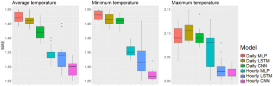
Figure 4.
Box plots of the best performance among the different input lengths in the metropolitan area, Seoul.
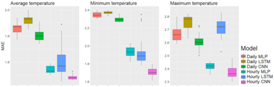
Figure 5.
Box plots of the best performance among the different input lengths in the mountainous area, Daegwalleong.
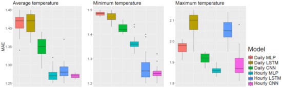
Figure 6.
Box plots of the best performance among the different input lengths in the coastal area, Seongsan.
5.1. Experimental Setup
Several factors may affect the accuracy of temperature forecasting with neural networks, so we employed neural a network with the following four parts:
- Model structure: We selected three neural network models to compare models their suitability for the temperature forecasting. The models we tested were MLP, LSTM, and CNN.
- Time unit of input data: We selected two different units of input data to predict daily temperatures for comparison: daily, which was the same as the target data, and hourly, which was more detailed than the target.
- Length of input data: We selected five separate lengths of input data to determine the lengths of historical data needed to forecast the next-day temperature. The data lengths were 1 day and 3, 5, 10, and 30 days.
- Region: We selected three regions in South Korea to understand the impacts of regional characteristics on temperature forecasting: Seoul as a metropolitan area, Daegwalleong as a mountainous area, and Seongsan as a coastal area.
We summarize the factors and levels for each vector in Table 14. Note that each model performs the pointwise forecasts for the location of the ASOS station in each region, and the input variables collected only from the station that corresponds to the target variable were used for these tasks.
The structures of actual input and target data used in the experiments are as follows. First, both daily and hourly input data are constructed by employing the data described in Section 4.3.1 and Section 4.3.2, respectively. An hourly data contains 15 weather variables for every hour in the length of input data and a daily data contains these variables for every day. For MLP, an input is flattened to a vector with the length of the number of weather variables, 15, multiplied by the time steps, the length of input for daily data and 24 times of the length of input for hourly data. LSTM receives a sequence with the length of the time steps and each element of the sequence is a vector containing the weather variables. Finally, for CNNs, an input data is a two-dimensional matrix whose dimensions correspond to the number of weather variables and the number of time steps. For instance, for the temperature forecasting using three days of hourly data, an input instance contains 1080 numerical weather values with 15 weather variables for 72 time steps. The input for MLP model is a 1080-dimensional vector, that for LSTM is a sequence of 15-dimensional vectors whose length is 72, and that for CNN is a rectangular matrix whose size is 72 by 15. Second, the target variables are the daily average, minimum, and maximum temperature after one day of the inputs.
The details of the experimental setup are as follows. We divided the entire ten years of data into batches of six years of data, two years of data, and another two years or data in sequential order to prevent information leakage [3,36,43]. We then used these three batches as training, validation, and test data, respectively. Since we employ information of several previous days from the target date, target values in the test data set may be used as inputs in training or validation data sets if we randomly split training, validation, and test sets. After splitting data sets, we randomize the order of instances in the training set. To optimize our models, we used an adaptive moment estimation optimizer with a learning rate of 0.00005 and set the mini-batch size to 4. To prevent over-fitting, we performed early stopping using the validation data set. All of the activation functions are in rectified linear units. To measure the accuracy of the models, we used mean absolute error (MAE) because it intuitively shows the differences between the actual and predicted temperatures. The mathematical loss function is shown in (11):
where is the number of instances, is the target value of -th instance, and is its predicted value.
We conducted additional experiments by combining the proposed method with recent approaches including multimodal learning, multitask learning, and input variables from other regions. First, we employed satellite images as additional inputs to the numerical meteorological data of the target region for forecasting temperature to apply multimodal learning to the proposed method. In this experiment, we added convolution layers that processes satellite images, and then concatenated it with the output of the convolution layer that processed the numerical weather data to perform forecasting temperature. The CNN model for multimodal learning has two sets of convolutional layers for two types of inputs, numerical weather data, and satellite images. The convolutional layers for satellite images consist of seven layers with 2 2 convolution filters with stride 2 and those for the numerical weather data are the same with the convolutional layers used for ordinary forecasting. After both types of inputs are processed into intermediate output values by the corresponding convolutional layers, these intermediate outputs are flattened and concatenated. Then, this concatenated vector is transmitted to the fully connected layers, whose structure is the same with the CNN models in Table 4, Table 5 and Table 6, to predict the target temperature. The satellite image data was taken from 12-h period observations over three years from 2015 to 2017 [44]. Therefore, the numerical weather data was also used for the corresponding period. In addition, the number of satellite images used for prediction coincides with the length of the numerical inputs. For example, six consecutive satellite images are employed for forecasting temperatures for the models that use three-day numerical inputs. We divided the entire three years of data into batches of two years of data, six months of data, and another six months of data in sequential order [3,36,43]. We then used these three batches as training, validation, and test data, respectively.
Second, we studied if global variables such as input variables from other regions can improve the temperature forecasting performance. We used the numerical meteorological variables collected from the stations other than the target region for these experiments. For instance, when forecasting the temperatures in Seoul, the input variables of Daegwallyeong and Seongsan are input together with the data of Seoul. For this experiment, we used three convolution layers of the same structure of the CNN model and passed the convolution by receiving input data from Seoul, Daegwallyeong and Seongsan areas, respectively. After that, we concatenate it into a fully connected layer with the same structure as the above experiment and then forecast the temperature in a specific area.
Third, temperatures in each region may be closely related to those in each other. Therefore, we verified the effect of shared information between the temperature forecasting tasks using deep multitask learning that learns related tasks simultaneously. We used input variables from all three regions as in the case for global variables. Using the input variables, four multitask learning models were constructed as follows: (1) a model forecasting average temperatures in three regions, (2) a model forecasting minimum temperatures in three regions, (3) a model forecasting maximum temperatures in three regions, (4) a model forecasting the average, minimum, and maximum temperatures in all three regions.
5.2. Experimental Results
To check the significance of the forecasting performance, we performed the experiments 25 times for each setting with random initialization of model weights. Table 15, Table 16 and Table 17 show the mean MAEs with standard deviations for each setting and each of the three regions for the average, minimum, and maximum temperature forecasts. For instance, when we predicted the minimum temperature in Seoul 25 times using three-day time unit data, the mean and standard deviation for the MAE were 1.246 and 0.041, respectively. To aid in understanding, Figure 4, Figure 5 and Figure 6 show box plots of the best performance among the different input time lengths for each setting with the boldfaced values in Table 15, Table 16 and Table 17.
We explain the experimental results for each factor as follows. First, for model structures, the CNN performed best with both daily and hourly input data; in the metropolitan area using hourly input data, the CNN showed means of MAE 1.295, 1.246, and 2.001 for average, minimum, and maximum temperature, respectively. MLP showed averages MAEs of 1.344, 1.353, and 2.065, and the LSTM averages of MAE were 1.380, 1.299, and 2.055, both respectively. The standard deviations were 0.029, 0.041, and 0.022 for the CNN; 0.027, 0.024, and 0.037 for the MLP, and 0.181, 0.087, and 0.130 for the LSTM; the LSTM showed larger standard deviations than those with the CNN and MLP. As Figure 4 shows, the first quartiles of LSTM using hourly input data are lower than those of the MLP using the same data. However, the gap between the first and third LSTM quartiles was large, and there were a few outliers. In contrast, the CNN showed robust performance in both means and standard deviations.
In terms of time units of the input data, the hourly data showed better performance than did the daily data. In particular, the difference was prominent when forecasting average and minimum temperatures. In Figure 4, Figure 5 and Figure 6, the box plots show that the first quartiles of results using daily input data are higher than the third quartiles of results using hourly data.
For time length of input data, based on the results boldfaced in Table 15, Table 16 and Table 17, the best results were 22 times for 1 day, 11 times for 3 days, 14 times for 5 days, 5 times for 10 days, and 2 times for 30 days. We obtained most of the best results when the length of the input data ranged from 1 to 5 days. However, it was interesting to note that the LSTM model showed the best results when we used longer input data, and the MLP showed the best results with short data lengths. With the CNN, hourly input data, and forecasting the coastal area, longer input data showed the best performance. In contrast, shorter input data were best for forecasting in the mountainous area. Therefore, the time length of the input data can be interpreted to be affected not only by the artificial neural network model but also by the region.
Overall, the models performed best in Seongsan, the coastal area, and the worst in Daegwallyeong, the mountainous area. The forecasting performance best to worst was for the coastal area, the metropolitan area, and then the mountainous area. With the CNN with hourly input data, the best average MAEs for the coastal area were 1.210, 1.234, and 1.900, and the best averages for the mountainous area were 1.481, 1.700, and 2.367. Therefore, the differences in forecasting accuracy across regions are apparent in each region.
For the three temperatures, we forecasted, predicting the maximum temperature was obviously the most difficult task. In Table 15, Table 16 and Table 17, all maximum temperatures under the same setting give worse results than those for the average and minimum temperatures. We found a clear pattern in the experimental results that predicting the maximum temperatures in the mountainous area was difficult, and we interpreted the causes of these results as follows. Table 18 shows the daily differences in temperatures between yesterday and today for 10 years, called differencing. The differences in daily temperature increase the forecasting difficulty because there were high daily temperature differences in the maximum temperatures in the mountainous region.
Table 18.
Average of daily temperature absolute differences.
In this regard, CNN using hourly input data, which showed the best results, reported interesting results as follows. In the coastal region, unlike the other regions, the CNN with hourly input data performed best with longer input data. We interpret this to reflect that a CNN extracts valid information from earlier times for forecasting temperatures in areas with relatively lower daily differences, as shown in Table 18. In contrast, in areas with larger differences, the CNN appeared to employ relevant, more recent input data. Therefore, it is necessary to set appropriate time lengths for the input data according to the daily differences in a region to improve forecasting performance.
In addition, we performed a comparative experiment on the preprocessing methods of missing values by accident. In the case of the existing experiments, as mentioned in 4.2.1, missing values by accident were replaced with data from the previous point, which is one of the widely used preprocessing methods for time series data. Another typical method is linear interpolation, which interpolates missing values using data before and after the point in time. We performed forecasting temperatures using the data preprocessed in each method to compare the two preprocessing methods. The experiment was conducted with CNN using three days of hourly data that showed the best overall performance. After 25 experiments were repeated for each forecasting temperature task, we performed one-tailed t-tests and the results are shown in Table 19. The experimental results are the average MAE and standard deviation of each method and the p-value of the one-tailed t-tests. Since the smallest p-value was 0.176, the two methods did not show statistically significant difference. We interpreted this result as follows. The 10-year hourly data consists of a total of 87,648 rows and each variable have only less than 100 missing values on average. Also, the linear interpolation may not be usable in actual cases because it uses future values to impute missing values.
Table 19.
Forecasting results, represented using the MAE for two imputation methods.
The followings are the experimental results of combining the proposed method with recent approaches. All experiments on multimodal learning, global variables, and multitask learning were conducted with CNN-based models using three-day hourly inputs. First, Table 20 show the average MAEs with standard deviations for multimodal learning. The best results are boldfaced. The multimodal learning using satellite image with numerical weather data did not improve overall performance. Excluding the average temperature in the Seongsan region, the average MAEs were higher than the model using the numerical weather data. In other words, providing additional satellite image was not effective to forecast temperature. We interpreted the causes of the result as follows. First, the time interval between satellite images is so large that it could not improve the temperature forecasting performances. Utilizing higher-frequent satellite images may be helpful in this case. Second, the satellite images may not be suitable for other weather forecasting tasks such as rainfall prediction and solar radiation which are directly affected by the cloud situation, rather than the temperature forecasting.
Table 20.
Forecasting results, represented using the MAE for multimodal learning.
Second, Table 21 includes the results of temperature forecasting with input variables from other regions in the average MAEs with standard deviations. The experimental results with the global variables, the variables from all three regions, showed better results than those with the local variables, the input variables only from the target region, for the average and maximum temperature of Daegwallyeong area and the average, minimum, and maximum temperature of Seongsan area. Especially, the average MAE of the maximum temperature in Daegwallyeong area was improved from 2.461 to 2.370, and the average MAEs of average and maximum temperature in Seongsan area were improved from 1.210, 1.900 to 1.110, 1.781, respectively. It can be considered that the CNN model extracted useful information from input data of other regions when forecasting a specific region. It is noteworthy that the forecasting performance is improved even for the maximum temperatures, which has high forecasting difficulty.
Table 21.
Forecasting results of, represented using the MAE for global variables and multitask learning.
Finally, the average MAEs with standard deviations of multitask learning are also shown in Table 21 where the best results are boldfaced. The multitask model for forecasting the average temperatures in three regions simultaneously improved the forecasting performance of Seongsan. The multitask model for maximum temperatures also improved forecasting performance in Seongsan. Finally, the multitask model, which forecasted nine temperatures simultaneously, performed better at maximum temperature in Daegwalleong and minimum and maximum temperatures in the Seongsan. The multitask learning showed better performance for tasks equal to single task with global conditions compared to single task with local conditions. Therefore, the improvement of average temperature performance in Daegwallyeong was mainly due to the effect of global conditions. However, the maximum temperature in Daegwallyeong and all temperatures in Seongsan can be interpreted as the effect of shared information between related tasks as well as the effects of global condition.
To sum up the results, hourly input data are more effective for daily temperature forecasting than daily input data. Therefore, we conclude that when forecasting daily temperatures, detailed hourly data provide better information than daily data. Here, a CNN with hourly input data outperformed an MLP and LSTM. The length of time of the input data depended on both the model and the region, and the regions showed significant differences in forecasting difficulty. In addition, it was effective to perform forecasting temperature with input data of different regions together and learn related forecasting tasks simultaneously using multitask learning in some cases.
6. Conclusions
We performed daily average, minimum, and maximum temperature forecasting with daily and hourly numerical weather data using neural network models. The hourly input, a more detailed time unit than the target data, had never been studied before. In order to process the detailed and abundant input data, we approached it from the perspective of two-dimensional signal processing using diverse neural network models, MLP, LSTM, and CNN. In particular, a CNN had never been used to forecast temperatures using numeric weather data. In addition, we conducted a comparison study to analyze temperature forecasting tasks affected by various factors. We found that the CNN showed better forecasting performance than did the MLP and LSTM. For time units of the input data, hourly input data worked better than daily input data in most cases. The time length of the input data depended on both the model and the region. To sum up the experimental results, depending on the target region, the CNN model using hourly input data of appropriate time length showed the best performance. In addition, using data from different regions together and multitask learning were effective in improving temperature forecasting performance in some cases.
Future researchers can incorporate loss balancing algorithms for multitask learning to improve the performance of challenging tasks. To improve the performance of difficult tasks including maximum temperature, researchers could consider dynamic task prioritization [45] and weighted loss function [46]. In addition, the proposed procedure in this study, including the usage of high-frequent inputs and variables from other regions, and employment of multitask learning algorithms, can be applied to forecast other weather variables including amount of water precipitation, solar radiation quantity, wind speed, and so forth.
Author Contributions
S.L. responsible the whole part of the paper (Conceptualization, methodology, analysis and writing—original draft preparation) Y.-S.L. responsible methodology, and review and editing and Y.S. responsible methodology, review and editing, and supervision. All authors have read and agreed to the published version of the manuscript.
Funding
The first and second authors (S.L. and Y.-S.L.) of this research were supported by National Research Foundation of Korea, grant number 2017R1E1A1A03070102 and the third author (Y.S.) of this research was supported by the Dongguk University Research Fund of 2017.
Conflicts of Interest
The authors declare no conflict of interest.
References
- Mathur, S.; Kumar, A.; Chandra, M. A feature based neural network model for weather forecasting. Int. J. Comput. Intell. 2008, 4, 209–216. [Google Scholar]
- Notton, G.; Voyant, C.; Fouilloy, A.; Duchaud, J.L.; Nivet, M.L. Some Applications of ANN to Solar Radiation Estimation and Forecasting for Energy Applications. Appl. Sci. 2019, 9, 209. [Google Scholar] [CrossRef]
- Haidar, A.; Verma, B. Monthly Rainfall Forecasting Using One-Dimensional Deep Convolutional Neural Network. IEEE Access 2018, 6, 69053–69063. [Google Scholar] [CrossRef]
- Hippert, H.; Pedreira, C.; Souza, R. Combining Neural Networks and ARIMA Models for Hourly Temperature Forecast. In Proceedings of the IEEE-INNS-ENNS International Joint Conference on Neural Networks, Hong Kong, China, 1–6 June 2008. [Google Scholar]
- Sharma, N.; Sharma, P.; Irwin, D.; Shenoy, P. Predicting solar generation from weather forecasts using machine learning. In Proceedings of the IEEE International Conference of Smart Grid Communications, Brussels, Belgium, 17–20 October 2011. [Google Scholar]
- Kim, T.; Ko, W.; Kim, J. Analysis and Impact Evaluation of Missing Data Imputation in Day-ahead PV Generation Forecasting. Appl. Sci. 2019, 9, 204. [Google Scholar] [CrossRef]
- Qin, Q.; Lai, X.; Zou, J. Direct Multistep Wind Speed Forecasting Using LSTM Neural Network Combining EEMD and Fuzzy Entropy. Appl. Sci. 2019, 9, 126. [Google Scholar] [CrossRef]
- Durai, V.; Bhardwaj, R. Evaluation of statistical bias correction methods for numerical weather prediction model forecasts of maximum and minimum temperatures. Nat. Hazards 2014, 73, 1229–1254. [Google Scholar] [CrossRef]
- Maqsood, I.; Khan, M.; Abraham, A. An ensemble of neural networks for weather forecasting. Neural Comput. Appl. 2004, 13, 112–122. [Google Scholar] [CrossRef]
- Shi, X.; Chen, Z.; Wang, H.; Yeung, D.Y. Convolutional LSTM Network: A Machine Learning Approach for Precipitation Nowcasting. In Proceedings of the 28th International Conference on Neural Information Processing Systems, Montreal, QC, Canada, 7–12 December 2015. [Google Scholar]
- Scher, S. Toward Data-Driven Weather and Climate Forecasting: Approximating a Simple General Circulation Model With Deep Learning. Geophys. Res. Lett. 2018, 45, 12616–12622. [Google Scholar] [CrossRef]
- Candy, B.; Saunders, R.W.; Ghent, D.; Bulgin, C.E. The Impact of Satellite-Derived Land Surface Temperatures on Numerical Weather Prediction Analyses and Forecasts. J. Geophys. Res. Atmos. 2017, 122, 9783–9802. [Google Scholar] [CrossRef]
- Reichstein, M.; Camps-Valls, G.; Stevens, B.; Jung, M.; Denzler, J.; Carvalhais, N. Deep learning and process understanding for data-driven Earth system science. Nature 2019, 566, 195–204. [Google Scholar] [CrossRef]
- Pathak, J.; Wikner, A.; Fussell, R.; Chandra, S.; Hunt, B.R.; Girvan, M.; Ott, E. Hybrid forecasting of chaotic processes: Using machine learning in conjunction with a knowledge-based model. Chaos 2018, 28, 041101. [Google Scholar] [CrossRef] [PubMed]
- Goswami, K.; Patowary, A. Monthly Temperature Prediction Based on Arima Model: A Case Study in Dibrugarh Station of Assam, India. Int. J. Adv. Res. Comput. Sci. 2017, 8, 292–298. [Google Scholar]
- Papacharalampous, G.; Tyralis, H.; Koutsoyiannis, D. Predictability of monthly temperature and precipitation using automatic time series forecasting methods. Acta Geophys. 2018, 66, 807–831. [Google Scholar] [CrossRef]
- Nyatuame, M.; Agodzo, S. Stochastic ARIMA model for annual rainfall and maximum temperature forecasting over Tordzie watershed in Ghana. J. Water Land Dev. 2018, 37, 127–140. [Google Scholar] [CrossRef]
- Khotanzad, A.; Davis, M.; Abaye, A.; Maratukulam, D. An Artificial Neural Network Hourly Temperature Forecaster with Applications in Load Forecasting. IEEE Trans. Power Syst. 1996, 11, 870–876. [Google Scholar] [CrossRef]
- Acharya, U.; Fujita, H.; Oh, S.; Hagiwaram, Y.; Tan, J.; Adam, M. Application of deep convolutional neural network for automated detection of myocardial infarction using ECG signals. Inf. Sci. 2017, 415, 190–198. [Google Scholar] [CrossRef]
- Park, S.; Lee, J.; Son, Y. Predicting Market Impact Costs Using Nonparametric Machine Learning Models. PLoS ONE 2016, 11, e0150243. [Google Scholar] [CrossRef]
- Abdel-Hamid, O.; Mohamed, A.; Jiang, H.; Deng, L.; Penn, G.; Yu, D. Convolutional Neural Networks for speech recognition. IEEE ACM Trans. Audio Speech Lang. Process. 2014, 22, 1533–1545. [Google Scholar] [CrossRef]
- Graves, A.; Mohamed, A.; Hinton, G. Speech recognition with deep recurrent neural networks. In Proceedings of the IEEE International Conference on Acoustics, Speech and Signal Processing, Vancouver, BC, Canada, 26–30 May 2013. [Google Scholar]
- Acharya, U.; Oh, S.; Hagiwara, Y.; Tan, J.; Adeli, H. Deep convolutional neural network for the automated detection and diagnosis of seizure using EEG signals. Comput. Biol. Med. 2018, 100, 270–278. [Google Scholar] [CrossRef]
- Tsiouris, K.; Pezoulas, V.; Zervakis, M.; Konitsiotis, S.; Koutsoris, D.; Fotiadis, D. A Long Short-Term Memory deep learning network for the prediction of epileptic seizures using EEG signals. Comput. Biol. Med. 2018, 99, 24–37. [Google Scholar] [CrossRef]
- Son, Y.; Noh, D.J.; Lee, J. Forecasting trends of high-frequency KOSPI200 index data using learning classifiers. Expert Syst. Appl. 2012, 39, 11607–11615. [Google Scholar] [CrossRef]
- Son, Y.; Byun, H.; Lee, J. Nonparametric machine learning models for predicting the credit default swaps: An empirical study. Expert Syst. Appl. 2016, 58, 210–220. [Google Scholar] [CrossRef]
- Yildirim, O. A novel wavelet sequence based on deep bidirectional LSTM network model for ECG signal classification. Comput. Biol. Med. 2018, 96, 189–202. [Google Scholar] [CrossRef] [PubMed]
- Hochreiter, S.; Schmidhuber, J. Long Short-Term Memory. Neural Comput. 1997, 9, 1735–1780. [Google Scholar] [CrossRef] [PubMed]
- LeCun, Y.; Bottou, L.; Bengio, Y.; Haffner, P. Gradient-based learning applied to document recognition. Proc. IEEE 1998, 86, 2278–2324. [Google Scholar] [CrossRef]
- Lawhern, V.; Solon, A.; Waytowich, N.; Gordon, S.; Hung, C.; Lance, B. EEGNet: A compact convolutional neural network for EEG-based brain-computer interfaces. J. Neural Eng. 2016, 15, 056013. [Google Scholar] [CrossRef]
- Kim, K.; Kim, D.; Noh, J.; Kim, M. Stable Forecasting of Environmental Time Series via Long Short Term Memory Recurrent Neural Network. IEEE Access 2018, 6, 75216–75228. [Google Scholar] [CrossRef]
- Xiao, C.; Chen, N.; Hu, C.; Wang, K.; Xu, Z.; Cai, Y.; Xu, L.; Chen, Z.; Gong, J. A spatiotemporal deep learning model for sea surface temperature field prediction using time-series satellite data. Environ. Model. Softw. 2019, 120, 104502. [Google Scholar] [CrossRef]
- Han, M.; Feng, Y.; Zhao, X.; Sun, C.; Hong, F.; Liu, C. A Convolutional Neural Network Using Surface Data to Predict Subsurface Temperatures in the Pacific Ocean. IEEE Access 2019, 7, 172816–172829. [Google Scholar] [CrossRef]
- Li, Z.; Wang, K.; Li, C.; Zhao, M.; Cao, J. Multimodal Deep Learning for Solar Irradiance Prediction. In Proceedings of the International Conference on Internet of Things and IEEE Green Computing and Communications and IEEE Cyber, Physical and Social Computing and IEEE Smart Data, Atlanta, GA, USA, 14–17 July 2019. [Google Scholar]
- Qiu, M.; Zhao, P.; Zhang, K.; Huang, J.; Shi, X.; Wang, X.; Chu, W. A Short-Term Rainfall Prediction Model Using Multi-task Convolutional Neural Networks. In Proceedings of the IEEE International Conference on Data Mining, New Orleans, LA, USA, 18–21 November 2017. [Google Scholar]
- Dorado-Moreno, M.; Navarin, N.; Gutierrez, P.A.; Prieto, L.; Sperduti, A.; Salcedo-Sanz, S.; Hervas-Martinez, C. Multi-task learning for the prediction of wind power ramp events with deep neural networks. Neural Netw. 2020, 123, 401–411. [Google Scholar] [CrossRef]
- Korea Meteorological Administration. Available online: https://data.kma.go.kr (accessed on 26 November 2018).
- Korea Evaluation of Contribution of Meteorological Observation Data to Weather Forecasts. 2018. Available online: https://kma.go.kr (accessed on 12 February 2020).
- Ahn, J.B.; Lee, J.; Im, E.S. The Reproducibility of Surface Air Temperature over South Korea Using Dynamical Downscaling and Statistical Correction. J. Meteorol. Soc. Jpn. 2012, 90, 493–507. [Google Scholar] [CrossRef]
- National Weather Service. Available online: https://www.weather.gov/asos/ (accessed on 12 February 2020).
- Korea National Geographic Information Institute. Available online: https://www.ngii.go.kr/eng/main.do (accessed on 29 October 2019).
- Lee, M.; Moon, S.; Yoon, Y.; Kim, Y.; Moon, B. Detecting Anomalies in Meteorological Data Using Support Vector Regression. Adv. Meteorol. 2018, 2018. [Google Scholar] [CrossRef]
- Pan, C.; Tan, J. Day-Ahead Hourly Forecasting of Solar Generation Based on Cluster Analysis and Ensemble Model. IEEE Access 2019, 7, 112921–112930. [Google Scholar] [CrossRef]
- Korea National Meteorological Satellite Center. Available online: https://nmsc.kma.go.kr (accessed on 3 February 2020).
- Guo, M.; Haque, A.; Huang, D.; Yeung, S.; Fei-Fei, L. Dynamic Task Prioritization for Multitask Learning. In Proceedings of the European Conference on Computer Vision, Munich, Germany, 8–14 September 2018. [Google Scholar]
- Chen, Z.; Badrinarayanan, V.; Lee, C.; Rabinovich, A. GradNorm: Gradient Normalization for Adaptive Loss Balancing in Deep Multitask Networks. In Proceedings of the International Conference on Machine Learning, Stockholm, Sweden, 10–15 July 2018. [Google Scholar]


© 2020 by the authors. Licensee MDPI, Basel, Switzerland. This article is an open access article distributed under the terms and conditions of the Creative Commons Attribution (CC BY) license (http://creativecommons.org/licenses/by/4.0/).