Abstract
The laminar, natural convective flow of a micropolar nanofluid in the presence of a magnetic field in a square porous enclosure was studied. The micropolar nanofluid is considered to be an electrically conductive fluid. The governing equations of the flow problem are the conservation of mass, energy, and linear momentum, as well as the angular momentum and the induction equations. In the proposed model, the Darcy–Brinkman momentum equations with buoyancy and advective inertia are used. Experimentally obtained forms of the dynamic viscosity, the thermal conductivity, and the electric conductivity are employed. A meshless point collocation method has been applied to numerically solve the flow and transport equations in their vorticity-stream function formulation. The effects of characteristic dimensionless parameters, such as the Rayleigh and Hartmann numbers, for a range of porosity and solid volume fraction of Al2O3 particles in a water-based micropolar nanofluid on the flow and heat transfer in the cavity are investigated. The results indicate that the intensity of the magnetic field significantly affects both the flow and the temperature distributions. Moreover, the addition of nanoparticles deteriorates the heat-transfer efficiency under specific conditions.
1. Introduction
Magnetohydrodynamics (MHD) focuses on electrically conducting fluids, which move under the influence of a magnetic field. The induced electrical current interacts with the magnetic field to produce a body force acting on the fluid. The interaction between the flow field (fluid velocity) and the externally applied magnetic field gives rise to a magnetic (induced) field inside the fluid. The MHD-oriented research field has become an important branch of fluid dynamics. The study of MHD flow applies to many industrial and engineering systems, such as nuclear reactors, heat exchangers [1], home ventilation systems, cooling of electronic equipment, solar energy collectors, nuclear reactors, chemical processing equipment, geothermal reservoirs, magnetic behavior of plasmas in fusion reactors, petroleum industries [2], boundary layer control in aerodynamics, crystal growth, and ship propulsion [3], to name a few [4,5].
Furthermore, MHD has been studied by many researchers, and considerable effort has been directed toward MHD flow combined with heat transfer. In fact, many authors have studied the effects of magnetic field on mixed, natural, and forced convective heat-transfer problems. Chandra and Gosh [6] studied the effect of a magnetic field on an electrically conducted viscoelastic fluid, reporting on the flow decrease through the increase in the magnetic field strength. Jha [7] studied the effects of natural convection and applied magnetic field on the Couette flow of an electrically conducting fluid between two parallel plates. Duwairi and Duwairi [8] reported on the thermal radiation heat transfer effects on the MHD–Rayleigh flow. Di Piazza and Ciofalo [9] studied the magneto-convection in a lead–lithium mixture, showing that a magnetic field, directed perpendicular to the temperature gradient, produced a complex three-dimensional flow pattern. Kenjeress and Hanjalic [10] studied the Rayleigh–Benard convection, subjected to various magnetic fields, over a range of Rayleigh and Hartmann numbers, and reported on the impact of the orientation and distribution of externally applied magnetic fields on the heat transfer and the flow regime (convective structures) in thermal convection of electrically conductive fluids. They studied the flow laminarization over specific range of Hartmann numbers. Through laminarization, it is possible to control thermal convection and associated heat transfer.
Over the last few decades, there has been a growing interest in the heat-transfer properties of nanofluids. Nanofluids are engineered colloids, i.e., a mixture of a base fluid (usually water, oil, or glycerin) and nanosized solid particles [11,12,13,14,15]. Nanofluids exhibit novel properties that make them potentially useful in many applications in heat transfer, including fuel cells, pharmaceutical processes, engine cooling/vehicle heating, and heat exchangers. They possess increased thermal conductivity and heat-transfer coefficients, compared to the base fluid. However, a critical parameter for their suitability in many applications is their rheological behavior.
In numerous computational studies, nanofluids are modeled as single-phase fluids, having altered physical properties compared to the ones of the base fluid [16,17,18]. Mahmoudi and Abu-Nada [19] studied the combined effect of the magnetic field and the nanofluids’ behavior on natural convection within a square cavity. They reported that the presence of the nanoparticles has an adverse effect on the heat transfer at a high-volume fraction of the nanoparticles. Makinde [20] studied the effects of viscous dissipation. Their results show that the increase of the volume fraction of nanoparticles enhances the heat-transfer rate. However, intensification of viscous dissipation has a negative effect in the heat-transfer rate. Jani [21] studied the free convection heat transfer in rectangular enclosure. The obtained results showed that the rate of heat transfer increased only at low Rayleigh numbers. This contradicting behavior has not been studied with adequate consideration and is one of the objectives of the present work.
Additionally, intensive research is conducted in order to comprehend the underlying physics of nanofluids, particularly the phenomena related to their increased thermal conductivity, compared to the thermal conductivity of the base fluid. Seven main mechanisms have been proposed toward a more comprehensive understanding of their physical properties, and, among them, nanoparticle microrotation seems to play a crucial role [22,23,24]. A mathematical model that takes into consideration the microrotation has been used in the study of Bourantas and Loukopoulos [25]. Therein, authors applied the micropolar flow theory to model the nanofluid. They used an experimentally obtained formula for the thermal conductivity and the dynamic viscosity of the nanofluids, and compared the numerical results with experimental data, with the accuracy being excellent.
Considerable effort has been directed toward heat-transfer studies for natural convection in porous media [26,27,28,29,30]. Oztop [31] studied the heat transfer with natural convection of an inclined partially cooled rectangular enclosure filled with a porous medium. Natural convection heat transfer in a cavity saturated with porous media in the presence of magnetic fields is a new branch of thermo-fluid mechanics. Shehadeh and Duwairi [32] studied MHD natural convective heat transfer in a rectangular enclosure filled with a porous medium, considering Joule and viscous heating effects.
In the present study, the micropolar flow theory is utilized to study the natural convection of a micropolar nanofluid in a square cavity filled with a porous medium and subjected to a magnetic field. Given its practical interest in the engineering and medical fields, including blood flow and purification [24], exportation of geothermal energy, purifications of metals, and solar heating systems [33], the topic needs to be further explored. The work on natural convection in a square cavity filled by a micropolar nanofluid [25] is extended here to account for the applied magnetic field in the presence of a porous medium. We developed a robust, efficient, and accurate meshless strong form collocation solver to numerically solve the governing flow equations. The latter are a set of nonlinear, fully coupled partial differential equations (PDEs), which express the conservation of mass, energy, linear momentum, and angular momentum, in addition to the magnetic induction. In the present study, the velocity–vorticity formulation is used, in order to avoid the problem of determining the pressure boundary conditions explicitly. To this end, a sophisticated five-step algorithm is implemented numerically. The criterion for terminating the algorithm is the normalized root-mean-square error of all field variables becoming less that a predefined value. An advanced Discretization Corrected Particle Strength Exchange (DC PSE) interpolation method is reformulated to calculate the spatial derivatives up to the second order in an Eulerian framework.
The physical aim of this study is to investigate the effect of the magnetic field magnitude and the intensity of the flow field, as well as the volume fraction of the nanoparticles and the permeability of the medium, on the convective heat transfer of an Al2O3/water nanofluid. The streamlines, temperature, microrotation, and vorticity contours are presented for characteristic ranges of solid volume fractions (0 ≤ φ ≤ 0.03), Hartmann numbers (0 ≤ Ha ≤ 1000), Rayleigh numbers (106 ≤ Ra ≤ 5 × 10⁸), and porosity of the medium (0.5 ≤ ε ≤ 0.7). In the proposed model, the Darcy–Brinkman momentum equations with buoyancy and advective inertia terms are used. The microrotation vector is affected by the presence of the particles and the pore walls. For this reason, a single-fluid equation in a porous setting is implemented, incorporating the effective microrotational properties of the nanofluid, using volume-averaging in representative elementary volumes (REVs), avoiding the necessity of considering the effect of the detailed pore structure on the form of the equation itself. Similar manipulation has been applied for the presence of the magnetic field. In this way, a magnetic field term is not required in the transport equation for the microrotation vector.
The rest of the paper is as follows. In Section 2, the governing equations of the proposed micropolar nanofluid model are presented, while the validation of the numerical method used for the solution of the flow equations and of the proposed micropolar nanofluid model, as well, are depicted in Section 3. In Section 4, the heat-transfer performance of a micropolar nanofluid enclosed in a rectangular cavity is studied. For all simulations, pure water is considered as the base fluid, with Pr = 6.2. Finally, in Section 5, the conclusions complete the paper.
2. Problem Formulation
In the present study, we consider the viscous, laminar, incompressible, natural convective flow in a square porous enclosure of length (L) filled with a micropolar Al2O3/water nanofluid in the presence of a magnetic field. The geometry and the configuration of the system are schematically shown in Figure 1.
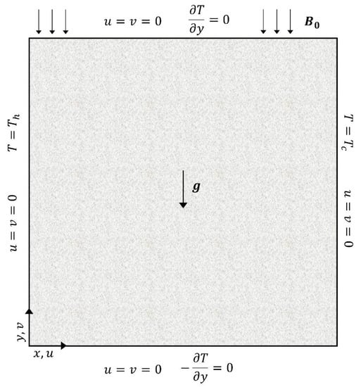
Figure 1.
Geometry and boundary conditions of the problem.
The top and bottom walls are insulated, and the fluid is isothermally heated and cooled at the left and right vertical walls at uniform temperatures, Th and Tc, respectively. In the case of natural convection, the buoyancy, which is a result of local fluid density variations due to temperature differences, is the dominant driving force, and the flow is permeated by an applied uniform external magnetic field, , in the direction of strength, . The fluid is in thermal equilibrium with the porous medium; the physical properties of the fluid are assumed constant, except of the density in the buoyancy force, which is calculated by using the Boussinesq approximation. We consider a granular porous medium of glass spheres. The thermophysical properties for the nanofluid and the glass spheres are listed in Table 1.

Table 1.
Thermophysical properties of water, alumina nanoparticles, and glass spheres, namely, the density (), the heat capacity (), the thermal conductivity (), the thermal expansion coefficient (), and the electric conductivity () [34,35,36].
The fluid is hydrodynamically, thermally, and electrically isotropic. No-slip and impermeable boundary conditions are imposed on all boundaries. Joule heating, viscous dissipation, pressure work, and Hall effects are neglected, as they are assumed negligible.
From Ohm’s law, the current density, J, relates to the electric field, E, as follows:
where is the electrical conductivity, and is the superficial velocity vector, with u and v being the velocity components along x and y axes, respectively. Using Ampere’s law, , we get the following:
omitting the inclusion of electromagnetic waves propagation and neglecting displacement currents, is the magnetic permeability (the nanofluid is assumed to have the same magnetic permeability with that of the base fluid). Using Faraday’s law and after algebraic manipulation, the magnetic induction equation is written as follows [37]:
Micropolar fluid theory was introduced by Eringen [38] as a generalization of the Navier–Stokes equations. Micropolar theory examines the microstructure of the fluid, along with the inertial characteristics of the particles, which can rotate under the influence of local forces. Microrotation, which is a new kinematic variable introduced in Eringen’s model, is related the rotation of the particles. The micropolar vector describes the rotation of the particles contained in a volume element [22,23]. A detailed analysis of the micropolar fluid flow theory is presented in [24].
In the proposed model, the Darcy–Brinkman momentum equations with buoyancy and advective inertia terms are used (see Equation (5)). The quantities that appear in the equations are the classical averaged quantities for flows in porous media. On the other hand, Equation (6), which is the transport equation for the microrotation vector, n, represents quantities which are not averaged directly. It is applied within the pores and, therefore, the correct equation to be used would be an averaged form of these equations. The microrotation vector is affected by the presence of particles and pore walls; however, a single-phase fluid equation in a porous setup was used, incorporating the effective microrotational properties of the particulate phase of the nanofluid, assuming volume-averaged values in porous representative elementary volumes (REVs) and avoiding the incorporation of the details of the pore structure in the expression of the angular momentum equation itself. The same concept applies for the presence of the magnetic field, which should affect the properties of the micropolar nanofluid due to their intrinsic nature; however, the magnetic field is not required to be implemented as a term in the transport equation for n, since its influence on the flow can be regarded solely through the particular term in the linear momentum equation. Thus, the governing equations of the problem, i.e., the conservation of mass, energy, and linear and angular momentum, as well as the induction equation, are written as Equations (4)–(8) [39,40,41].
The boundary conditions for the natural convection problem studied are set to the following:
is the pressure, is the fluid temperature, is the superficial microrotation vector, is the induced magnetic field, and is the acceleration due to gravity. is the density, is the dynamic viscosity, is the vortex viscosity, is the spin-gradient viscosity, and is the micro-inertia density. For the present simulation study, it is further assumed that has the following form, as proposed in [42,43].
The effective density for the nanofluid is given by an Effective Medium Theory (EFM) approach [30]:
with being the volume fraction of the nanoparticles. The effective dynamic viscosity for the nanofluid is given by the following:
which was measured experimentally by Pak and Cho [44]. The heat capacity of the nanofluid, along with the effective heat capacity of the medium, are given as follows [34]:
where ε is the porosity of the medium. The effective thermal diffusivity for the nanofluid is as follows:
while the thermal expansion coefficient of the nanofluid can be determined as follows:
The thermal conductivity of the nanofluid was calculated experimentally [44] and is given by the following:
The electrical conductivity of the alumina nanofluid, for the range of volume fractions used (), was calculated experimentally [35]:
The effective thermal conductivity, and the effective electrical conductivity, , of the porous medium can be calculated by the Maxwell correlation [39]:
The Carman–Kozeny relationship was chosen for the permeability of the medium [36]:
where is the average diameter of the glass spheres, considered here as . The total length of the cavity is .
Since pressure boundary conditions are inherently difficult to be defined with the present meshless method, the velocity–vorticity formulation was used. Taking the curl of the vorticity definition, , and using the continuity equation (Equation (4)), a vector Poisson equation can be used to correlate the vorticity and velocity fields (Equation (22)). The curl operator applies to the linear momentum conservation equation, Equation (5), and with the application of , , following the vorticity and microrotation definitions, and the mass conservation , one gets Equation (23). Additionally, the magnetic potential, , is used, given as , which satisfies the solenoidal nature of the magnetic field , (). Thus, and , where it is assumed that , with being the z-unit vector, as expected in two-dimensional (x, y) fields. Therefore, vector Equation (7) can be replaced by the scalar Equation (24). Finally, in two-dimensional flows, taking into account all previous assumptions, the governing equations in the velocity–vorticity formulation can be written as follows:
The following non-dimensional variables are introduced:
for the case of two-dimensional flows. Moreover, considering all previous assumptions, the final form of the equations is written as follows:
The dimensionless boundary conditions are:
where is the microrotation number, is the Prandtl number, is the magnetic Prandtl number, is the Rayleigh number, is the Hartmann number, and is the Darcy number. The Nusselt number can be expressed as follows:
while the average Nusselt number is defined as follows:
3. Numerical Method
The steady-state flow equations were numerically solved by using a meshless point collocation method [45,46]. The intermediate velocity, , computed from the Poisson equations for the velocity components (Equations (28) and (29)), did not satisfy the continuity equation. Therefore, the velocity field was updated, using the velocity correction method [47,48]. Assuming that the velocity correction () is irrotational, a correction potential, , can be defined as . The correction potential should satisfy a Poisson-type equation to satisfy the continuity equation.
The updated velocity, is calculated as . Following this, we briefly describe the solution procedure applied, placing emphasis on the calculation of the convective terms and on the imposition of Neumann boundary conditions.
3.1. Solution Procedure
The governing equations for the magnetic potential, the temperature, the microrotation and the vorticity (Equations (28)–(33)) can be expressed compactly as follows:
where is a differential operator; accounts for ; and is the right-hand side of the equation. All the field functions considered in Equation (38) are written in bold, since they are column vectors of dimensions , and is the total number of nodes (interior and boundary) used to represent the spatial domain. The notation, , defines the iteration step. For easier convergence, the convective term in the step is expressed as . For the variables under consideration, the operator and the right-hand side vector are given by the following equations:
The solution procedure commences with an initial guess for all the field variables, , , and . The algorithmic steps in the solution procedure may be ordered as follows:
- Step 1: Compute the intermediate velocity components, through Equations (28) and (29), using vorticity values at the previous step (for the first iteration, the prescribed initial conditions are used).
- Step 2: Compute the correction potential and update the velocity field ().
- Step 3: Solve Equations (30) and (31) for the magnetic potential and temperature. Then, calculate the magnetic field components and , along with the temperature gradient .
- Step 4: Solve the coupled equations for the microrotation and vorticity, Equations (32) and (33), using the updated magnetic field and temperature gradient.
- Step 5: Repeat Steps 1–4, until the normalized root-mean-square error NRMSE() of all field variables becomes less that a predefined value (e.g., 10−5).
The Discretization Corrected Particle Strength Exchange (DC PSE) method was implemented for the calculation of the derivatives [49] of the unknown field functions up to the second order. DC PSE was originally introduced as a Lagrangian particle-based solution method. The method has been reformulated [47] to numerically solve partial differential equations in Eulerian frameworks. The DC PSE interpolation method relies on Particle Strength Exchange (PSE) operators, i.e., kernel functions that approximate differential operators which conserve particle strength in particle–particle interactions. The PSE method was first introduced by Degond and Mas-Gallic [50] for diffusion and convection–diffusion problems, while Eldredge et al. [51] extended the method to compute approximations of arbitrary derivatives. Details on the DC PSE method can be found in [47].
3.2. Vorticity Boundary Conditions
Several formulae, based on finite difference methods, for the imposition of vorticity boundary values [52], usually referred to as local, were developed. Vorticity values on the boundaries were computed, using vorticity values of interior nodes, avoiding the involvement of boundary nodes. The most commonly used formula was Thom’s formula. Unfortunately, the application of these formulas in physical applications had limited success.
Global vorticity boundary conditions are more accurate, since both boundary and interior nodes are involved in their computation. In the present study, the DC PSE differential operators were applied for the computation of the vorticity boundary conditions [45,53]. In the DC-PSE-meshless collocation context, computing and imposing vorticity boundary conditions were considered as an interpolation problem. Using the updated velocity components from Step 2, we computed and , the updated vorticity values, (in the entire spatial domain, including the boundaries):
The vorticity values computed are used as boundary condition for Step 4, Equation (33).
3.3. Zero Flux Temperature Boundary Conditions
Frequently, for natural convection flow problems, Neumann boundary conditions (no-flux boundary conditions) are encountered, given as follows:
where is the unit normal vector of the boundary, and is the unknown scalar field function at the boundary (the temperature in the present case). We imposed such Neumann boundary conditions, using interior nodes, only in the support domain of the nodes with Neumann boundary conditions, shown in Figure 2, when computing the derivatives in Equation (44).
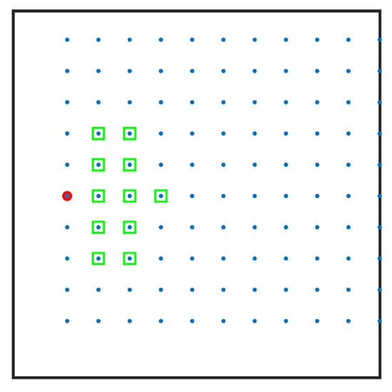
Figure 2.
Outline of the support domain used for imposing no-flux boundary conditions. A boundary node is denoted with a red circle, and the corresponding nodes in its support domain with green squares.
Boundary nodes having only interior nodes in their support domain allow the direct computation of the values on the boundary nodes based on known values of interior nodes and, thus, decoupling the Neumann boundary conditions. For a two-dimensional system with unit normal vector , the derivatives that appear in the Neumann boundary conditions are estimated by using the DC PSE method, with the following expression at each boundary node, :
with and being the weights of the first-order spatial derivatives. The Neumann boundary condition for node becomes the following:
allowing the computation of the value that has to be imposed at the boundary node as follows:
4. Results and Discussion
For the flow case studies considered here, the microrotation number, is set to , since it provides results that are closer to the experimental findings [25]. The Prandtl number is set to , and the magnetic Prandtl to .
4.1. Code Verification
In the present simulations, uniform Cartesian grids with increasing nodal resolution are used, ranging from up to . A grid-independent numerical solution was obtained by a grid of resolution, as seen in Figure 3. The average Nusselt number () on the left vertical wall (hot wall) was computed for validation purposes. The average Nusselt number for the natural convection in the square porous cavity is presented for , and two different values of and . For higher accuracy, a denser grid consisting of nodes was used. The accuracy of the proposed scheme was tested against verified numerical results obtained for MHD natural convection in a square cavity [54] (Table 2).
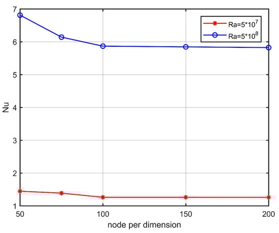
Figure 3.
Convergence analysis for Nuave along the hot wall. Variation with Ra.
Table 2.
Average Nusselt numbers at the hot wall for characteristic Grashof and Hartmann numbers obtained by the present method (underlined) and [54].
Table 2 shows the average Nusselt number on the left vertical wall, as presented in the work of Ece et al. (underline values) [54] and the results of the proposed method. In these cases, the medium consisted only of the fluid (), the Hartmann number ranged from , and the Grashof number varied in the range . The Grashof number is inherently related to the Rayleigh and Prandtl numbers through the relationship . The comparative results are in good agreement.
4.2. Effect of Porosity (ε)
Initially, the flow regime in the case of varying porosity of the medium was examined. The porosity is strongly related to the permeability of the system (Equation (21)). By increasing porosity, the permeability and the Darcy number of the porous medium increases. In the present simulations, the volume fraction of nanoparticles was set to , the Rayleigh number to , and the Hartmann number to .
In all porosity values considered, a central clockwise-rotating flow pattern was formed along the diagonal of the square enclosure, having two anticlockwise circulating regions in both the upper-left and lower-right parts of the diagonal, as shown in Figure 4. Three flow regions were formed, a hot region bounded between the left and top walls, a cold region between the right and bottom walls, and a third one along the diagonal area where temperature varies. By increasing porosity, the flow patterns intensify (higher stream function values), and the anticlockwise rotating cells tend to dominate the flow. Isotherms expand gradually, as stronger circulation favors concentration of isotherms lines. The microrotation isolines form a central vortex diagonally, increasing in length as the porosity increases. Vorticity variations are observed at the upper-right and lower-left edges of the cavity, whereas their thickness decreases and the intensity of the vorticity increases with increasing porosity.
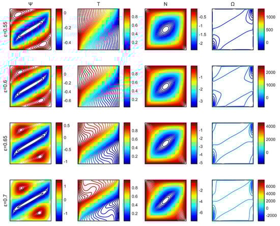
Figure 4.
Stream function (), temperature ( ), microrotation ( ), and vorticity ( ) contours for a range of porosities of the medium.
Figure 5 shows the average Nusselt number () versus porosity () for Hartmann numbers and . In both Ha cases, the average Nusselt number increases with increasing porosity, as the flow intensity increases. For zero Hartmann number (), the increase of the Nusselt number is more pronounced, highlighting the inhibitory effect of the magnetic field on the flow field and the heat distribution. The local Nusselt number along the hot wall is proportional to the temperature gradient (see Equation (35)), and higher values of the average Nusselt number indicate that an increased amount of energy was transferred from the heat source to the nanofluid and, eventually, to the porous medium.
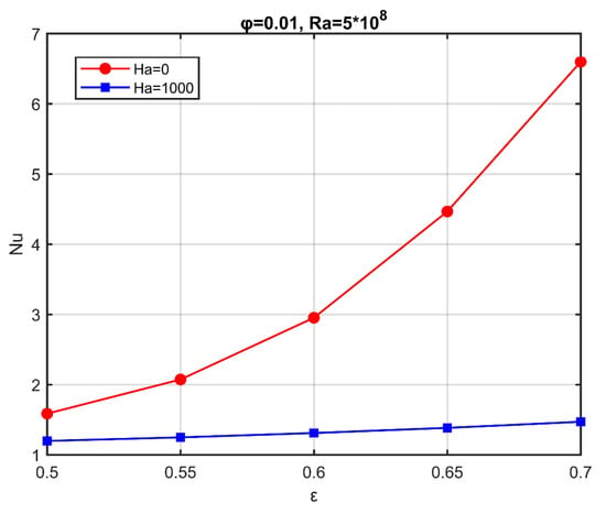
Figure 5.
Average Nusselt number variation with porosity for two characteristic Hartmann numbers. .
4.3. Effect of the Hartmann Number (Ha)
Next, the flow regime in the case of different Hartmann numbers was investigated, related with the intensity of the applied magnetic field. The volume fraction was set to , the Rayleigh number , and the porosity to .
After the onset of the magnetic field, notable variations in the stream function, the microrotation, and the temperature contours were observed. The anticlockwise rotating vortex formations gradually disappeared, and two secondary rotating cells (having low stream function values) appeared initially along the diagonal, shifting horizontally and disappearing as the Hartmann number increased (Figure 6). Boundary layers (Hartmann layers) were established on the vertical walls of the cavity. Microrotation contours formed a vortex that moved toward the center of the cavity as the Hartmann number increased. Initially, the isotherms swirled according to the flow field, and as the Hartmann number increased, they became parallel to the vertical walls. The vorticity formed two vortices at the vertical walls for high values of the Hartmann number.
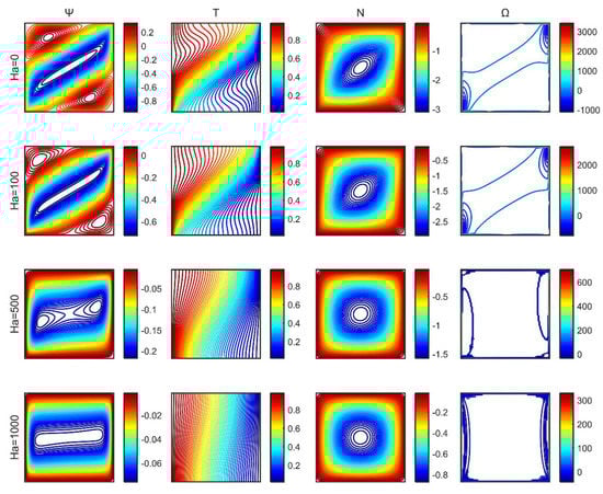
Figure 6.
Stream function (), temperature ( ), microrotation ( ), and vorticity ( ) contours for a range of Hartmann numbers.
A decrease in the heat transfer was observed, along with an increase in the intensity of the magnetic field, through the variation of the Nuave along the hot wall (Figure 7). The average Nusselt number decreased with the increase in the Hartmann number. The decrease of the average Nusselt number was more evident for elevated values of the Rayleigh number.
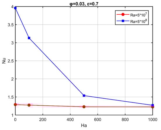
Figure 7.
Average Nusselt number as a function of the Hartmann number, for characteristic Rayleigh numbers; .
4.4. Effect of the Rayleigh Number (Ra)
Cases with varying Rayleigh number were also under investigation. For these simulations, the volume fraction was kept at , while the porosity was kept at . The Hartmann number was set to .
For the low Rayleigh values considered, a large clockwise rotating vortex was formed, as shown in Figure 8. The fluid rose from the left vertical wall, the location of the heat source, and flowed downward along the right vertical wall. By increasing the Rayleigh number, isotherms expanded gradually, as they emerged from the heat source and reached the rest of the walls. Furthermore, the flow regime became stronger, and the streamlines were intensified. For higher values of the Rayleigh number (), the two anticlockwise rotating formations appeared in the stream function contour, and the distribution of the isothermal lines changed from conduction-controlled to convection-dominated. For small values of the Rayleigh number, a minute variation on the vorticity was observed near the walls of the cavity. Microrotation contours had a central vortex at the middle of the cavity that elongated diagonally for elevated values of the Rayleigh number.
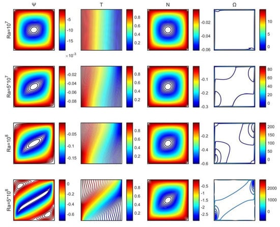
Figure 8.
Stream function (), temperature ( ), microrotation ( ), and vorticity ( ) contours for a range of Rayleigh numbers.
The dependence of the average Nusselt number, on is shown in Figure 9 for two values, and two porosities of the medium, while the volume fraction was set to . The increase of resulted in an increase of . For , a smaller increase of the Nusselt number was observed, as the presence of the magnetic field had a negative effect on the strength of the flow field.
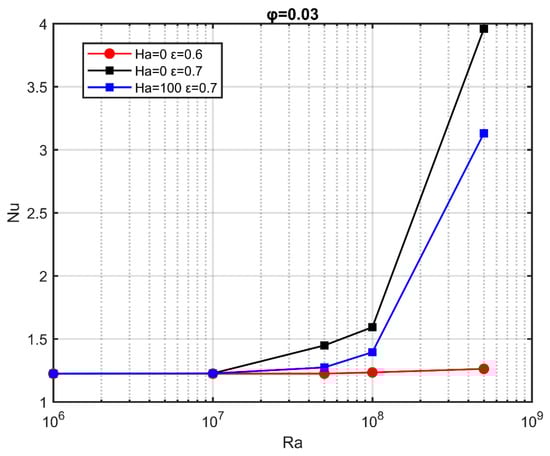
Figure 9.
Average Nusselt number as a function of the Rayleigh number, for characteristic Hartmann numbers;
4.5. Effect of the Volume Fraction (φ)
The influence of the volume fraction of the Al2O3 nanoparticles on the flow regime and the heat-transfer properties of the nanofluid was under examination. The Hartmann number was set equal to , the Rayleigh number to , and the porosity to . In the present simulations, the nanoparticles volume fraction, , ranges from to .
The volume fraction of the nanoparticles added in the base fluid alters the heat-transfer properties of the nanofluid. When nanoparticles were added, the thermal and electrical conductivity of the base fluid (water) increased. Even with low (1%–5% volumetric) concentration of the nanoparticles, the thermal conductivity increased by 10%–20%.
As the nanoparticles volume fraction increased, the intensity of the flow regime became weaker, and that of the flow field decreased, Figure 10. This is attributed to the increase of the electrical conductivity, as the effect of the applied magnetic field on the nanoparticles becomes stronger. The temperature contours follow the alteration of the flow field, and the microrotation isolines form a vortex at the center of the cavity.
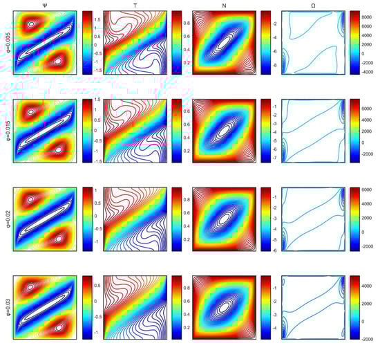
Figure 10.
Stream function (), temperature ( ), microrotation ( ), and vorticity ( ) contour plots for characteristic volume fractions of the nanoparticles.
The dependence of Nuave on the solid volume fraction is shown in Figure 11. At low-flow conditions, , conduction is the dominant mechanism for heat transfer, and the Nusselt number increases as the volume fraction of the particles increases, as expected by the increased thermal conductivity offered by the nanoparticles with respect to the base fluid thermal properties. As the flow conditions intensify, convection is at play, and increases, as well, provided the volumetric concentration of nanoparticles is constant. However, at elevated flow conditions, , even in the absence of a magnetic field, the Nusselt number is reduced as the volume fraction of the nanoparticles increases, and this slope declines as the Rayleigh number increases. As the Hartmann number increases, the Nusselt number recedes further.

Figure 11.
Average Nusselt number as a function of the volume fraction of nanoparticles, for characteristic Hartmann and Rayleigh numbers, and .
The decrease in the heat transfer with the addition of nanoparticles under elevated flow conditions was not an anticipated result, given the intended purpose of nanofluids to increase the efficiency of thermal processes. However, similar behavior has been observed and reported in previous experimental [36] and numerical [21] investigations of the thermal behavior of buoyancy-driven nanofluids in rectangular enclosures. In [36], the Nusselt number of the base fluid in a porous medium was found to be higher than that of the nanofluid for elevated Rayleigh numbers. In [21], the Nusselt number decreased (~10–30%) with the addition of nanoparticles for high Rayleigh numbers. In the present case, the phenomenon was more intense (~50%) due to the additional presence of the porous medium. The nanofluid moved with additional hindrance through the pores, due to the quadratic increase of the effective fluid viscosity (Equation (11)), and an increase of the volume fraction reduced the fluid flow and, thus, the convection. Therefore, even though the thermal conductivity increased, the convective heat transfer was reduced, and the Nusselt number decreased. Moreover, in the case of an applied magnetic field, the decrease was steeper, since the magnetic field had a negative effect on the intensity of the flow field.
5. Conclusions
In the present work, the laminar, natural convective flow of an Al2O3-water micropolar nanofluid in a rectangular porous enclosure under the presence of a magnetic field was numerically investigated. The micropolar flow theory was applied and extended to study nanofluidic natural convection phenomena subjected to magnetic fields in the interior of porous media. The nanofluid was assumed hydrodynamically, thermally, and electrically isotropic. Moreover, it was assumed to be in constant thermal equilibrium with the porous medium. The governing equations were solved in the stream function–vorticity description. A robust, efficient, and accurate meshless strong-form solver was presented, to numerically solve the governing set of coupled partial differential equations. The steady-state equations were solved, using a meshless point collocation method for the discretization, and a five-step algorithm was developed. A reformulated DC PSE method was employed to calculate the derivatives of the unknown field functions up to the second order, in a Eulerian framework, with increased accuracy.
The flow characteristics and, thus, the convective heat transfer inside the enclosure were determined by the intensity of the magnetic field, the volume fraction of the nanoparticles, the porosity, and the strength of the flow field. Circulation and convection phenomena intensified with increasing Rayleigh numbers, though they were suppressed considerably by the presence of a strong magnetic field. Formation of rotating vortexes greatly influenced the temperature distribution. The average Nusselt number increased substantially with the Rayleigh number, since the circulation grew stronger. The magnetic field reduced the local Nusselt number considerably by the suppression of the convection currents. The porosity of the medium also affected the convective heat transfer. The average Nusselt number increased with increasing porosity, as the flow intensity increased. The addition of nanoparticles had either a negative or positive effect on the heat transfer, depending on the intensity of the flow field. For small Rayleigh numbers, the heat transfer increased due to a higher thermal conductivity. For large Rayleigh numbers, the decrease in the heat transfer was caused by the elevated viscosity of the nanofluid, which reduces the fluid flow and the heat convection mechanisms. This decrease in the heat transfer of the nanofluids under elevated flow conditions was not an anticipated result, given the intended purpose of nanofluids to increase the efficiency of thermal processes; however, it was corroborated by previous experimental [36] and numerical [21] observations. Furthermore, the very presence of the porous medium affected the heat transfer noticeably, as an increase in the effective viscosity of the fluid further impeded the nanofluid motion through the pores. The presence of the magnetic field intensified the phenomenon.
Author Contributions
Conceptualization, N.P.K., G.C.B., E.D.S., V.C.L., K.M., and V.N.B.; funding acquisition, N.P.K., K.M., and V.N.B.; methodology, N.P.K., G.C.B., E.D.S., and V.C.L.; project administration, K.M. and V.N.B.; software, N.P.K. and G.C.B.; supervision, K.M. and V.N.B.; validation, N.P.K., G.C.B., E.D.S., and V.C.L.; visualization, N.P.K.; writing—original draft, N.P.K. and G.C.B.; writing—review and editing, E.D.S., V.C.L., K.M., and V.N.B. All authors have read and agreed to the published version of the manuscript.
Funding
This research was funded by the Hellenic Foundation for Research and Innovation (HFRI ELIDEK), PhD scholarships 2017, with grant number 80264. Methods for transport simulations in porous materials were also financed by the project “Advanced Research Activities in Biomedical and Agroalimentary Technologies” (MIS 5002469), which is implemented under the “Action for the Strategic Development on the Research and Technological Sector”, funded by the Operational Programme “Competitiveness, Entrepreneurship and Innovation” (NSRF 2014-2020) and co-financed by Greece and the European Union (European Regional Development Fund). This research was also supported by the Australian Government through the Australian Research Council’s Discovery Projects funding scheme (project DP160100714).
Acknowledgments
Computational infrastructure was provided by the Institute of Chemical Engineering Sciences, Foundation for Research and Technology, Hellas (FORTH/ICE-HT).
Conflicts of Interest
The authors declare no conflict of interest.
References
- Melnikov, I.A.; Sviridov, E.V.; Sviridov, V.G.; Razuvanov, N.G. Experimental investigation of MHD heat transfer in a vertical round tube affected by transverse magnetic field. Fusion Eng. Des. 2016, 112, 505–512. [Google Scholar] [CrossRef]
- Mukhopadhyay, S. MHD boundary layer slip flow along a stretching cylinder. Ain Shams Eng. J. 2013, 4, 317–324. [Google Scholar] [CrossRef]
- Jang, J.; Lee, S.S. Theoretical and experimental study of MHD (magnetohydrodynamic) micropump. Sens. Actuators A Phys. 2000, 80, 84–89. [Google Scholar] [CrossRef]
- Ostrach, S. Natural convection in enclosures. J. Heat Transf. 1988, 110, 1175–1190. [Google Scholar] [CrossRef]
- Jani, S.; Amini, M.; Mahmoodi, M. Numerical study of free convection heat transfer in a square cavity with a fin attached to its cold wall. Heat Transf. Res. 2011, 42. [Google Scholar] [CrossRef]
- Ghosh, B.C.; Ghosh, N. MHD flow of a visco-elastic fluid through porous medium. Int. J. Numer. Methods Heat Fluid Flow 2001, 11, 682–698. [Google Scholar] [CrossRef]
- Jha, B.K. Natural convection in unsteady MHD couette flow. Heat Mass Transf. 2001, 37, 329–331. [Google Scholar] [CrossRef]
- Duwairi, H.M.; Duwairi, R.M. Thermal radiation effects on MHD-Rayleigh flow with constant surface heat flux. Heat Mass Transf. 2004, 41, 51–57. [Google Scholar] [CrossRef]
- Di Piazza, I.; Ciofalo, M. MHD free convection in a liquid-metal filled cubic enclosure. I. Differential heating. Int. J. Heat Mass Transf. 2002, 45, 1477–1492. [Google Scholar] [CrossRef]
- Kenjereš, S.; Hanjalić, K. Numerical simulation of magnetic control of heat transfer in thermal convection. Int. J. Heat Fluid Flow 2004, 25, 559–568. [Google Scholar] [CrossRef]
- Kakaç, S.; Pramuanjaroenkij, A. Review of convective heat transfer enhancement with nanofluids. Int. J. Heat Mass Transf. 2009, 52, 3187–3196. [Google Scholar] [CrossRef]
- Lee, J.-H.; Lee, S.-H.; Choi, C.; Jang, S.; Choi, S. A review of thermal conductivity data, mechanisms and models for nanofluids. Int. J. Micro Nano Scale Transp. 2011, 1, 269–322. [Google Scholar] [CrossRef]
- Eapen, J.; Rusconi, R.; Piazza, R.; Yip, S. The classical nature of thermal conduction in nanofluids. J. Heat Transf. 2010, 132. [Google Scholar] [CrossRef]
- Wong, K.V.; De Leon, O. Applications of nanofluids: Current and future. In Nanotechnology and Energy; Jenny Stanford Publishing: Singapore, 2017; pp. 105–132. [Google Scholar]
- Fan, J.; Wang, L. Review of heat conduction in nanofluids. J. Heat Transf. 2011, 133, 040801. [Google Scholar] [CrossRef]
- Putra, N.; Roetzel, W.; Das, S.K. Natural convection of nano-fluids. Heat Mass Transf. 2003, 39, 775–784. [Google Scholar] [CrossRef]
- Wen, D.; Ding, Y. Natural convective heat transfer of suspensions of titanium dioxide nanoparticles (nanofluids). IEEE Trans. Nanotechnol. 2006, 5, 220–227. [Google Scholar]
- Polidori, G.; Fohanno, S.; Nguyen, C.T. A note on heat transfer modelling of Newtonian nanofluids in laminar free convection. Int. J. Therm. Sci. 2007, 46, 739–744. [Google Scholar] [CrossRef]
- Mahmoudi, A.H.; Abu-Nada, E. Combined effect of magnetic field and nanofluid variable properties on heat transfer enhancement in natural convection. Numer. Heat Transf. Part A Appl. 2013, 63, 452–472. [Google Scholar] [CrossRef]
- Makinde, O.D. Effects of viscous dissipation and Newtonian heating on boundary-layer flow of nanofluids over a flat plate. Int. J. Numer. Methods Heat Fluid Flow 2013, 23, 1291–1303. [Google Scholar] [CrossRef]
- Jani, S.; Mahmoodi, M.; Amini, M.; Akbari, M. Free convection in rectangular enclosures containing nanofluid with nanoparticles of various diameters. 2014, 45, 145–169.
- Eringen, A.C. Theory of micropolar fluids. J. Math. Mech. 1966, 16, 1–18. [Google Scholar] [CrossRef]
- Eringen, A.C. Microcontinuum field Theories: II. Fluent Media; Springer Science & Business Media: Berlin/Heidelberg, Germany, 2001; Volume 2. [Google Scholar]
- Lukaszewicz, G. Micropolar Fluids: Theory and Applications; Springer Science & Business Media: Berlin/Heidelberg, Germany, 1999. [Google Scholar]
- Bourantas, G.C.; Loukopoulos, V.C. Modeling the natural convective flow of micropolar nanofluids. Int. J. Heat Mass Transf. 2014, 68, 35–41. [Google Scholar] [CrossRef]
- Baytas, A.C.; Pop, I. Free convection in oblique enclosures filled with a porous medium. Int. J. Heat Mass Transf. 1999, 42, 1047–1057. [Google Scholar] [CrossRef]
- Kramer, J.; Jecl, R.; Škerget, L. Boundary domain integral method for the study of double diffusive natural convection in porous media. Eng. Anal. Bound. Elem. 2007, 31, 897–905. [Google Scholar] [CrossRef]
- Kumari, M.; Nath, G. Unsteady natural convection from a horizontal annulus filled with a porous medium. Int. J. Heat Mass Transf. 2008, 51, 5001–5007. [Google Scholar] [CrossRef]
- Varol, Y.; Oztop, H.F.; Pop, I. Natural convection in a diagonally divided square cavity filled with a porous medium. Int. J. Therm. Sci. 2009, 48, 1405–1415. [Google Scholar] [CrossRef]
- Bourantas, G.C.; Skouras, E.D.; Loukopoulos, V.C.; Burganos, V.N. Heat transfer and natural convection of nanofluids in porous media. Eur. J. Mech. B Fluids 2014, 43, 45–56. [Google Scholar] [CrossRef]
- Oztop, H.F. Natural convection in partially cooled and inclined porous rectangular enclosures. Int. J. Therm. Sci. 2007, 46, 149–156. [Google Scholar] [CrossRef]
- Shehadeh, F.G.; Duwairi, H.M. MHD natural convection in porous media-filled enclosures. Appl. Math. Mech. 2009, 30, 1113–1120. [Google Scholar] [CrossRef]
- Kim, Y.J. Unsteady MHD convective heat transfer past a semi-infinite vertical porous moving plate with variable suction. Int. J. Eng. Sci. 2000, 38, 833–845. [Google Scholar] [CrossRef]
- Aminossadati, S.M.; Ghasemi, B. Natural convection cooling of a localised heat source at the bottom of a nanofluid-filled enclosure. Eur. J. Mech. B Fluids 2009, 28, 630–640. [Google Scholar] [CrossRef]
- Ganguly, S.; Sikdar, S.; Basu, S. Experimental investigation of the effective electrical conductivity of aluminum oxide nanofluids. Powder Technol. 2009, 196, 326–330. [Google Scholar] [CrossRef]
- Grobler, C.; Sharifpur, M.; Ghodsinezhad, H.; Capitani, R.; Meyer, J. Experimental study on cavity flow natural convection in a porous medium, saturated with an Al2O3 60% EG-40% Water nanofluid. In Proceedings of the 11th International Conference on Heat Transfer, Fluid Mechanics and Thermodynamics, Skukuza, South Africa, 20–23 July 2015; Volume 2015. [Google Scholar]
- Davidson, P.A. An Introduction to Magnetohydrodynamics; Cambridge University Press: Cambridge, UK, 2001. [Google Scholar]
- Eringen, A.C. Simple microfluids. Int. J. Eng. Sci. 1964, 2, 205–217. [Google Scholar] [CrossRef]
- Nield, D.A.; Bejan, A. Convection in Porous Media; Springer: Berlin/Heidelberg, Germany, 2013. [Google Scholar]
- Malashetty, M.S.; Shivakumara, I.S.; Kulkarni, S. The onset of Lapwood—Brinkman convection using a thermal non-equilibrium model. Int. J. Heat Mass Transf. 2005, 48, 1155–1163. [Google Scholar] [CrossRef]
- Zadravec, M.; Hriberšek, M.; Škerget, L. Natural convection of micropolar fluid in an enclosure with boundary element method. Eng. Anal. Bound. Elem. 2009, 33, 485–492. [Google Scholar] [CrossRef]
- Ahmadi, G. Self-similar solution of imcompressible micropolar boundary layer flow over a semi-infinite plate. Int. J. Eng. Sci. 1976, 14, 639–646. [Google Scholar] [CrossRef]
- Rees, D.; Pop, I. Free convection boundary-layer flow of a micropolar fluid from a vertical flat plate. IMA J. Appl. Math. 1998, 61, 179–197. [Google Scholar] [CrossRef]
- Pak, B.C.; Cho, Y.I. Hydrodynamic and heat transfer study of dispersed fluids with submicron metallic oxide particles. Exp. Heat Transf. 1998, 11, 151–170. [Google Scholar] [CrossRef]
- Bourantas, G.; Skouras, E.; Loukopoulos, V.; Nikiforidis, G. Meshfree point collocation schemes for 2d steady state incompressible navier-stokes equations in velocity-vorticity formulation for high values of reynolds number. Comput. Model. Eng. Sci. 2010, 59, 31–63. [Google Scholar]
- Bourantas, G.C.; Skouras, E.D.; Loukopoulos, V.C.; Nikiforidis, G.C. An accurate, stable and efficient domain-type meshless method for the solution of MHD flow problems. J. Comput. Phys. 2009, 228, 8135–8160. [Google Scholar] [CrossRef]
- Bourantas, G.C.; Cheeseman, B.L.; Ramaswamy, R.; Sbalzarini, I.F. Using DC PSE operator discretization in Eulerian meshless collocation methods improves their robustness in complex geometries. Comput. Fluids 2016, 136, 285–300. [Google Scholar] [CrossRef]
- Zahab, Z.E.; Divo, E.; Kassab, A.J. A localized collocation meshless method (LCMM) for incompressible flows CFD modeling with applications to transient hemodynamics. Eng. Anal. Bound. Elem. 2009, 33, 1045–1061. [Google Scholar] [CrossRef]
- Schrader, B.; Reboux, S.; Sbalzarini, I.F. Discretization correction of general integral PSE Operators for particle methods. J. Comput. Phys. 2010, 229, 4159–4182. [Google Scholar] [CrossRef]
- Degond, P.; Mas-Gallic, S. The weighted particle method for convection-diffusion equations. I. The case of an isotropic viscosity. Math. Comput. 1989, 53, 485–507. [Google Scholar]
- Eldredge, J.D.; Leonard, A.; Colonius, T. A General deterministic treatment of derivatives in particle methods. J. Comput. Phys. 2002, 180, 686–709. [Google Scholar] [CrossRef]
- Weinan, E.; Liu, J.-G. Vorticity boundary condition and related issues for finite difference schemes. J. Comput. Phys. 1996, 124, 368–382. [Google Scholar]
- Bourantas, G.C.; Zwick, B.F.; Joldes, G.R.; Loukopoulos, V.C.; Tavner, A.C.; Wittek, A.; Miller, K. An explicit meshless point collocation solver for incompressible Navier-Stokes equations. Fluids 2019, 4, 164. [Google Scholar] [CrossRef]
- Ece, M.C.; Büyük, E. Natural-convection flow under a magnetic field in an inclined rectangular enclosure heated and cooled on adjacent walls. Fluid Dyn. Res. 2006, 38, 564–590. [Google Scholar] [CrossRef]
© 2020 by the authors. Licensee MDPI, Basel, Switzerland. This article is an open access article distributed under the terms and conditions of the Creative Commons Attribution (CC BY) license (http://creativecommons.org/licenses/by/4.0/).