Featured Application
The novel space–time radial polynomial basis function collocation method is first proposed for solving the backward heat conduction problems in this study. The proposed method can be applied to inverse problems with remarkably high accuracy; even severely ill–posed inverse problems under large noises are considered.
Abstract
In this article, a novel meshless method using space–time radial polynomial basis function (SRPBF) for solving backward heat conduction problems is proposed. The SRPBF is constructed by incorporating time-dependent exponential function into the radial polynomial basis function. Different from the conventional radial basis function (RBF) collocation method that applies the RBF at each center point coinciding with the inner point, an innovative source collocation scheme using the sources instead of the centers is first developed for the proposed method. The randomly unstructured source, boundary, and inner points are collocated in the space–time domain, where both boundary as well as initial data may be regarded as space–time boundary conditions. The backward heat conduction problem is converted into an inverse boundary value problem such that the conventional time–marching scheme is not required. Because the SRPBF is infinitely differentiable and the corresponding derivative is a nonsingular and smooth function, solutions can be approximated by applying the SRPBF without the shape parameter. Numerical examples including the direct and backward heat conduction problems are conducted. Results show that more accurate numerical solutions than those of the conventional methods are obtained. Additionally, it is found that the error does not propagate with time such that absent temperature on the inaccessible boundaries can be recovered with high accuracy.
1. Introduction
Solving a heat conduction problem is to determine temperature histories within the heat–conducting material [1,2,3]. Because the boundary conditions are often difficult to directly measure in industrial practices, the requirements for recovering the missing temperature render the problems into an inverse heat conduction problem [4]. The heat conduction problems are categorized into initial value problems, which have been extensively solved by meshless methods such as the method of fundamental solutions (MFS) [5], the radial basis function collocation method (RBFCM) [6,7,8], the element–free Galerkin method [9], the radial basis function finite difference method [10,11], and the local radial basis function–based differential quadrature method [12]. For time discretization in most published works, the time–marching methods such as the implicit, explicit, Crank–Nicolson or Runge–Kutta schemes are often adopted by approximating at each time interval [13,14,15].
Even though the success of numerical methods combined with the time–marching scheme is effective and easily implemented for dealing with heat conduction problems, limitations remain while utilizing the time–marching scheme including a small time interval for the convergence [16,17]. As a result, the time–marching methods for solving heat conduction problems may be computationally expensive. Recently, several numerical approaches based on the space–time scheme have been proposed [16,17,18,19,20]. Tezduyar et al. proposed the space–time finite element method (FEM) for the computation of fluid–structure interaction problems [17]. The space–time discontinuous Galerkin FEM has been proposed and applied for dealing with compressible Navier–Stokes equations as well as advection–diffusion problems [21,22]. Meanwhile, a collocation approach regarding space–time exponential basis functions for wave propagation problems, static and time harmonic elastic problems have been developed [23,24,25]. A new boundary–type meshfree technique incorporated with the space–time collocation scheme for modeling of heat conduction problems, as well as tide–induced groundwater response, have been also developed [20,26].
The space–time collocation approach using the radial basis function (RBF) can be traced back to Li and Mao [27]. Moreover, Hamaidi et al. developed the RBFCM using the space–time scheme for solving parabolic and hyperbolic equations [28]. Despite the success of the RBFs with the shape parameter as an effective numerical scheme for solving partial differential equations, the selection of the shape parameter may still dominate the accuracy of the results [29,30,31].
In this study, the pioneering work using the collocation scheme based on the space–time radial polynomial basis function (SRPBF) for modeling the transient heat conduction phenomena is first proposed. The randomly unstructured points are collocated in the space–time domain, where both boundary as well as initial data may be regarded as space–time boundary conditions. The SRPBF is constructed by incorporating time-dependent exponential function into the radial polynomial basis function. Since the SRPBF is nonsingular and infinitely smooth in nature, the shape parameter is not required in the proposed approach. Result comparison between the proposed method and that from the RBFCM with the time–marching scheme is conducted. The article is organized as follows. In Section 2, the SRPBF is introduced. In Section 3, we present the validation, accuracy, and convergence of the proposed approach. The comparison of results with the RBFCM with the time–marching scheme is then illustrated. Three examples of heat conduction are given to demonstrate the stability of our approach in Section 4. Findings are concluded in Section 5.
2. The Space–time Radial Polynomial Basis Function Collocation Method
The heat conduction problem is expressed as:
where is the thermal conductivity, x is the space–time coordinate, t is time, u is the temperature, is the Laplacian operator, and is the space–time domain. The space–time boundary condition is as follows:
where is the space–time boundary data, and is the space–time domain boundary.
The heat conduction problems are categorized into initial value problems, which may be dealed with utilizing the conventional time–marching methods such as the implicit, explicit, Crank–Nicolson or Runge–Kutta schemes in Euclidean space domain. Figure 1 demonstrates the Euclidean space domain for describing the one–dimensional (1D) heat conduction problem.
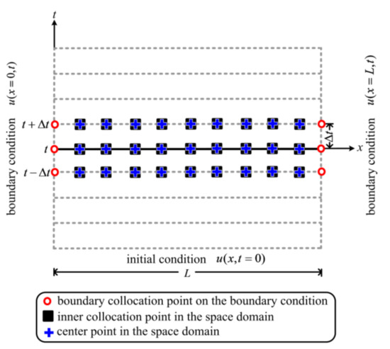
Figure 1.
Configuration of the collocation points for the direct heat conduction problem.
Different from the time–marching methods for dealing with the initial value problems, an innovative space–time collocation scheme is proposed in this study. The randomly unstructured source, boundary and inner points are collocated in the space–time domain, where both boundary as well as initial data may be regarded as space–time boundary conditions. The direct and backward heat conduction problems are converted into inverse boundary value problems such that the conventional time–marching scheme is not required.
For example, Equation (1) is the governing equation of a direct heat conduction problem (DHCP) with assigned space–time boundary conditions, as depicted in Figure 2a, for modeling the transient heat conduction phenomena. Figure 2 denotes the two–dimensional (2D) space–time domain where three sets of points including the boundary, source, and inner points are collocated in the 2D space–time domain. The 1D Euclidean space domain, therefore, transform into the 2D space–time area. The boundary as well as initial data are given on the three space–time boundaries, which transform a 1D transient problem to a 2D inverse boundary value problem. Equation (1) is the governing equation of a backward heat conduction problem (BHCP) as well. Similarly, to solve the BHCP, the boundary conditions and the final time condition on the space–time boundary have to be provided, as depicted in Figure 2b.
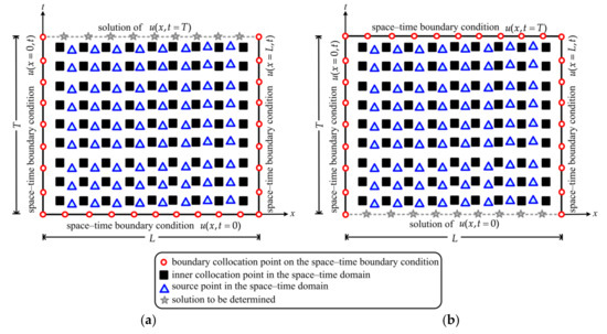
Figure 2.
Illustration of the space–time collocation scheme: (a) The direct heat conduction problem (DHCP); (b) The backward heat conduction problem (BHCP).
In this article, a new meshless method using the space–time radial polynomial is proposed. The temperature of the governing equation can be approximated utilizing the SRPBF as follows:
where , is the collocation points, which may be the boundary or inner points, is the source points, is the order of the SRPBF for approximating the solutions, and is the coefficient to be determined. In the preceding equations, the SRPBF is a smooth and nonsingular function without the shape parameter. The SRPBF is applied on the space–time domain in which time is considered as another independent dimension. The derivative of Equation (3) with respect to x is taken to acquire:
The derivative of Equation (4) with respect to x is taken to yield:
Taking the first derivative of Equation (3) with respect to t, we may yield the following equation:
Substituting Equations (5) and (6) into the governing equation can yield the following equation:
To determine the coefficients in Equation (7), we impose the approximate solution to satisfy the given partial differential equation with the boundary conditions. We then achieve the following equations:
where is a vector of unknown coefficients, is a matrix for the inner and boundary collocation points, is a vector of functions data at the inner and boundary points. The above equation can then be rewritten as follows:
where is a matrix for the inner collocation points, is a matrix for the boundary collocation points, is a vector of functions values at the inner collocation points, is a vector of boundary data with the size of , is the number of inner collocation points, is the number of boundary collocation points, and . To solve the system of equations, the commercial program MATLAB backslash operator is adopted.
To examine the stability of the proposed approach for solving the BHCP, the input data with noises are considered as:
where rand denotes the random number, is the final time input data with noises, is the noise data on accessible boundary, e is the noise level, which is expressed as , and s is the percentage of noise. As expressed in Equations (10) and (11), the noisy data are considered in the simulation of the BHCP.
To estimate the accuracy of the solutions, the root mean square error (RMSE) and maximum absolute error (MAE) are considered:
where and are the exact solution and numerical solution at the inner collocation points, respectively.
For the RBFCM, the center, boundary, and inner points are required to be collocated. The center point usually shares the same position with the inner collocation point in the RBFCM. Besides, the numbers of the inner and center points must be the same for generating the determinate system of simultaneous equations. With the consideration of time–marching scheme, we may have the collocation points for the 1D heat conduction problem as shown in Figure 1.
In this study, we propose a new idea for collocating the source points using two different schemes, namely the inner source collocation scheme and the outer source collocation scheme. The inner source collocation scheme is similar to that in the RBFCM, as depicted in Figure 2a. Different from the collocation scheme in the RBFCM, the center point is regarded as the source point in which the source and the inner points are collocated separately. Besides, the numbers of the source and the inner points are not necessary to be the same. It should be noted that all the collocation points are placed in the space–time domain. The boundary as well as initial conditions can, therefore, be turned into the space–time boundary conditions. Accordingly, the one-dimensional heat conduction initial value problem becomes the two–dimensional boundary value problem such that the conventional time–marching scheme is not applicable in the proposed method.
In this article, the idea of the outer source collocation scheme is motivated by the MFS. The conception of the MFS is to approximate numerical solutions through a fundamental solution by means of collocating the source points outside the boundary, where numerical solutions can be approximated adopting the linear combination of the nonsingular functions. Following the similar path, the sources of the outer source collocation scheme are collocated outside the domain, as depicted in Figure 3. The following equation is adopted for collocating the source points for the outer source collocation scheme:
where denotes the radiuses of the source points, denotes the angle of the source points, is the number of source points, denotes the dilation parameter and . The proposed two novel collocation schemes are investigated and applied to the example applications. Accuracy of the proposed collocation schemes are also discussed in the following section.
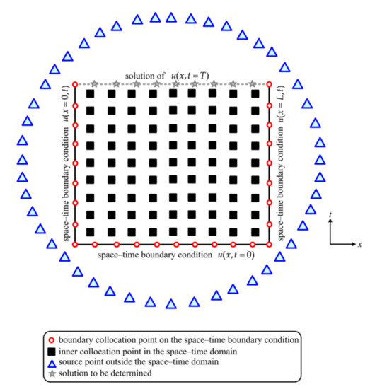
Figure 3.
The outer source collocation scheme.
3. Validation of the Proposed Method
3.1. Accuracy and Convergence Analysis
To investigate the accuracy of the source collocation scheme, a DHCP is carried out. The governing equation of the DHCP is expressed as Equation (1). The initial data are given by:
The boundary conditions on the right and left boundaries are described as the following equations:
We consider the following exact solution:
In this validation example, the space domain is 1 in length, the final elapsed time is 1, and the thermal conductivity is 1. The numbers of the inner collocation and source points are 400 and 100, respectively. The terms of the SRPBF and numbers of the boundary collocation points are listed in Table 1. To investigate the correctness of the source collocation scheme, the source points placed in and outside the 2D space–time domain are considered. For the inner source collocation scheme, the source points are placed in the 2D space–time domain, as depicted in Figure 2a. As for the outer source collocation scheme, we place the source points outside the 2D space–time domain, as depicted in Figure 3.

Table 1.
The maximum absolute error (MAE) of the proposed approach with the consideration of two source collocation schemes.
To illustrate the accuracy of the proposed approach, the MAE of the computed results is evaluated. The relationship between the terms of the SRPBF and the MAE with the consideration of the inner and outer source collocation schemes is demonstrated in Figure 4.
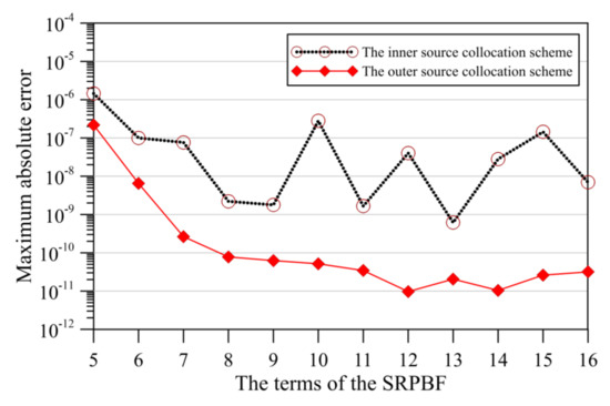
Figure 4.
The maximum absolute error versus the terms of the SRPBF.
For the inner source collocation scheme, it seems that the MAE of the order of 10−7 to 10−9 may be yielded when the terms of the SRPBF is in the range of 9 to 16. For the outer source collocation scheme, it is clear that the MAE of the order of 10−10 to 10−12 may be yielded when the terms of the SRPBF is in the range of 9 to 16. In addition, it seems that the terms of the SRPBF in the outer source collocation scheme are not very sensitive while the number of terms is greater than 8. From Figure 4, it appears that the computed results with high accuracy utilizing our approach with the consideration of the outer source collocation scheme can be acquired, which means that the source points collocated outside the 2D space–time domain may obtain more accurate results.
Since the position of the source point may affect the accuracy of the proposed approach, we further conduct an example to investigate the dilation parameter to the accuracy. In this example, the source points collocated at different locations outside the 2D space–time domain are utilized. The numbers of boundary collocation points, inner collocation points, and source point are considered to be 400, 400, and 100, respectively. The terms of the SRPBF are determined to be 8.
Figure 5 demonstrates the dilation parameter versus the MAE. It is found that highly accurate solutions in the order of 10−8 to 10−11 may be acquired when the dilation parameter ranges from 2 to 7, which indicates the location of the source points may be not sensitive to the accuracy of the outer source collocation scheme. Accordingly, we adopt the outer source collocation scheme for the following numerical examples.
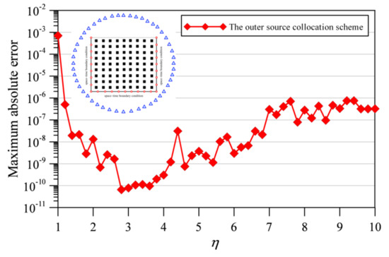
Figure 5.
The maximum absolute error versus the dilation parameter.
3.2. Comparison with the Radial Basis Function Collocation Method (RBFCM)
To compare the computed results with those obtained from the RBFCM based on the multiquadric (MQ) basis function using the time–marching scheme, we consider a 1D benchmark DHCP. The initial as well as boundary data are expressed as Equations (15) to (17). The exact solution as shown in Equation (18) is considered.
In this comparison example, the space domain is m in length, the final elapsed time is 2 h, and the thermal conductivity is 1 . To apply the conventional RBFCM based on the MQ function utilizing the time–marching method, the spatial and temporal discretizations have to be separately considered. For the spatial discretization, the length of the space is divided into segments, which have the equal length of . For the temporal discretization, the implicit difference scheme is adopted where the time interval () is 0.033 h. Figure 3 displays the collocation points of the 1D DHCP. We consider the number of boundary points in space domain and in time domain to be 80 and 120, respectively. Therefore, we have and , which are exactly the same with those in the conventional RBFCM using the time–marching scheme. As displayed in Figure 3, the numbers of the inner, source, and boundary points are 900, 100, and 200, respectively. The terms of the SRPBF and the dilation parameter are determined to be 11 and 4, respectively.
To validate the proposed approach, the computed results using our approach and the RBFCM utilizing the time–marching scheme are compared with the exact solution. Figure 6 presents the results computed using the conventional RBFCM, the proposed approach and the exact solution. It is clear that good agreement obtained by the both proposed approach and conventional RBFCM based on the MQ function using the time–marching scheme may be found.
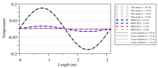
Figure 6.
Comparison of the computed results with the exact solution.
Figure 7 demonstrates the accuracy of our approach and the RBFCM based on the MQ function utilizing the time–marching method. The numerical solutions of the RBFCM based on the MQ function are computed utilizing the optimal shape parameter, where the shape parameter is considered to be 3. As for the proposed method, the terms of the SRPBF are 11. From Figure 7, it is found that the MAE of the proposed method is in the order of 10−7 to 10−11. As for the RBFCM based on the MQ function with the time–marching scheme, the MAE is in the order of 10−4 to 10−6. It is obvious that our approach may acquire better solutions than the RBFCM based on the MQ function with the time–marching scheme.
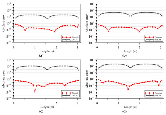
Figure 7.
Comparison of the error of the radial basis function collocation method (RBFCM) with the time–marching scheme and our approach at different time: (a) t = 0.5 h; (b) t = 1.0 h; (c) t = 1.5 h; (d) t = 2.0 h.
Figure 8 shows the relationship between the absolute error and simulation time. It is found that the absolute error may significantly increase with the simulation time in the time–marching method. The absolute error of the proposed approach, however, always remains in the order of 10−9 to 10−10 with the simulation time, which demonstrates that our approach may avoid the error propagation. It may be especially advantageous for DHCP requiring long simulation time.
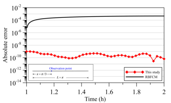
Figure 8.
Absolute error at observation point through time.
To compare the computational efficiency of the SRPBF with that of RBFCM, an efficiency analysis is carried out. From the results of the efficiency analysis, it is found that the central processing unit (CPU) time of the SRPBF and RBFCM is 121 (s) and 140 (s), respectively. Results obtained demonstrate that the proposed method may be more effective than the RBFCM.
4. Numerical Examples
4.1. The Direct Heat Conduction Problem (DHCP)
The first numerical example investigated is the modeling of a 1D DHCP. This example is to evaluate the correctness of our approach and to compare the computed results with those obtained from the space–time localized RBFCM [28]. The governing equation is written as Equation (1). The boundary values are described as follows:
The initial data are given by:
The solution is as:
In this 1D DHCP, the thermal conductivity is 1, the space domain is 1 in length, final time is 1, and . The final time and boundary data are provided on the top and lateral sides of the 2D space–time domain, respectively. The inner points are then provided in the 2D space–time domain. The numbers of the inner, source and boundary points are 900, 100, and 200, respectively. The terms of the SRPBF and the dilation parameter are determined to be 11 and 4, respectively. Figure 9 indicates the results computed with the exact solution. It is found that the temperature from our approach may achieve great agreement with the exact solution.
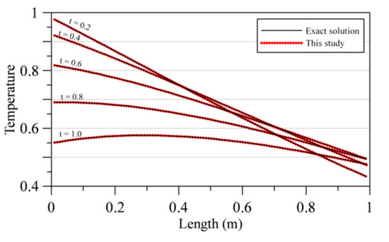
Figure 9.
Comparison of the computed temperature.
Hamaidi et al. (2016) have applied the space–time localized RBFCM to solve this DHCP [28]. The computed results of the proposed approach are then compared with those of the space–time localized RBFCM [28]. Table 2 depicts the MAE and RMSE adopting several boundary points in the time and space domain. From Table 2, the MAE and the RMSE using the proposed approach can reach to the order of 10−6 and 10−8. However, the MAE with different arrangements of the boundary points using the space–time localized RBFCM is of the order of 10−4 to 10−5. In addition, the RMSE with different arrangements of the boundary points associated with the space–time localized RBFCM may only reach to the order of 10−5 to 10−6 [28], as listed in Table 2. It is significant that the temperature with high accuracy can be acquired using the proposed approach.
Table 2.
The maximum absolute error (MAE) and root mean square error (RMSE) of the proposed approach and the space–time localized radial basis function collocation method (RBFCM).
4.2. The Backward Heat Conduction Problem (BHCP)
A 1D benchmark BHCP is considered in the second example. The governing equation, as written as Equation (1), is considered. The boundary values on the right and left boundaries are described as Equations (19) and (20). The boundary data at final time is:
The exact solution, as depicted in Equation (22), is adopted in the validation of BHCP. In this example, the thermal conductivity is 1, length of the space domain is 1, and . Since the assigned boundary data on the lateral boundaries are zero and the final time boundary data are small, this BHCP under investigation is a severely ill–posed case.
To examine the stability of our approach, we consider the 1D BHCP with different final elapsed time. The collocation scheme for the BHCP is shown in Figure 10. From Figure 10, the final time boundary data are assigned on the top side of the 2D space–time domain. The right and left boundary data are then assigned on the lateral sides of the 2D space–time domain. The numbers of the boundary, source and inner points are 750, 150, and 900, respectively. Parameters including the terms of the SRPBF and the dilation parameter in this BHCP are considered to be 11 and 4.
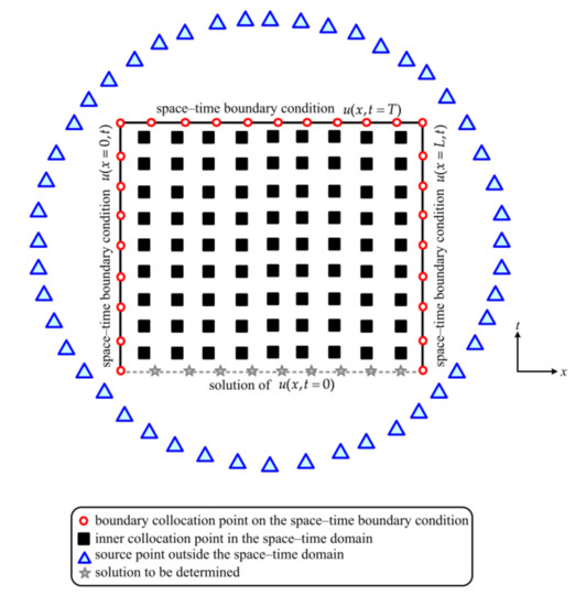
Figure 10.
The collocation scheme for the BHCP.
To illustrate the accuracy of our approach, the MAE and the RMSE of the computed results is evaluated by Equations (12) and (13). Table 3 shows the MAE and RMSE of our approach for solving the 1D BHCP with the consideration of different final elapsed time. The MAE of the numerical solutions with the consideration of final elapsed time is of the order of 10−6 to 10−8. The RMSE of the numerical solutions with the consideration of final elapsed time is of the order of 10−8 to 10−11. Figure 11 demonstrates the absolute error of our method with the consideration of different final elapsed time. From Figure 11, it seems that the recovered temperature with high accuracy may be yielded.
Table 3.
MAE and RMSE of the proposed approach for solving the BHCP.
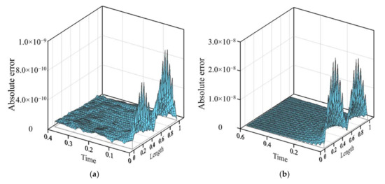
Figure 11.
The absolute error of the proposed method with the consideration of different final elapsed time: (a) T= 0.4; (b) T= 0.6; (c) T= 0.8; (d) T= 1.0.
4.3. The Benchmark BHCP
In the last numerical example, we consider a 1D benchmark BHCP [27]. The governing equation is expressed as Equation (1). The boundary conditions on the right and left boundaries are written as Equations (19) and (20). We consider the exact solution to be:
We consider the final elapsed time to be 0.25, length of the space domain to be 1, and thermal conductivity to be 1. Since the conventional RBFCM may provide only spatial approximation of the numerical solutions, it limits its application in inverse problems. Li and Mao was firstly proposed the RBFCM based on the global space–time MQ function [27]. The accuracy of our approach is then compared with that of the space–time MQ method developed by Li and Mao [27].
We collocate with the inner and boundary collocation points by using Equations (3) and (7). The boundary points are uniformly provided on the lateral and top sides of the 2D space–time domain. The numbers of boundary collocation points, inner collocation points, and source point are considered to be 121, 690, and 80, respectively. The terms of the SRPBF are determined to be 8.
The space–time MQ method has also been applied to solve this BHCP [27]. We then compare the accuracy of our approach with those of the space–time MQ method. Based on their results, the RMSE using the space–time MQ method can reach to the order of 10−7 [27]. However, the RMSE using our approach may reach to the order of 10−10. It appears that highly accurate initial temperature may be recovered utilizing our approach.
The input boundary conditions polluted by random noise are further considered. We consider the noise level to be 0, 0.01, 0.1, and 0.4, which are the same of those adopted by Li and Mao [27]. Figure 12 displays the estimated initial temperature with different noise level. The MAE for noise level 0, 0.01, 0.1, and 0.4 is 1.58 × 10⁻⁷, 4.41 × 10⁻⁵, 7.88 × 10⁻⁴, and 1.42 × 10⁻³, as depicted in Figure 13. It seems that high accurate initial temperature may be recovered utilizing our approach even when the measured data polluted by random noise are considered. Figure 14 demonstrates the RMSE versus different noise level. From Figure 14, the RMSE associated with the space–time MQ method is of the order of 10−2 to 10−3. However, the RMSE associated with our approach is of the order of 10−3 to 10−7. It appears that the RMSE associated with our method may provide better solutions than the space–time MQ method.
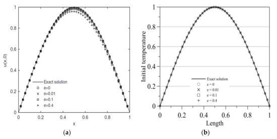
Figure 12.
The estimated initial temperature with noise level: (a) the space–time multiquadric (MQ) method; (b) this study.
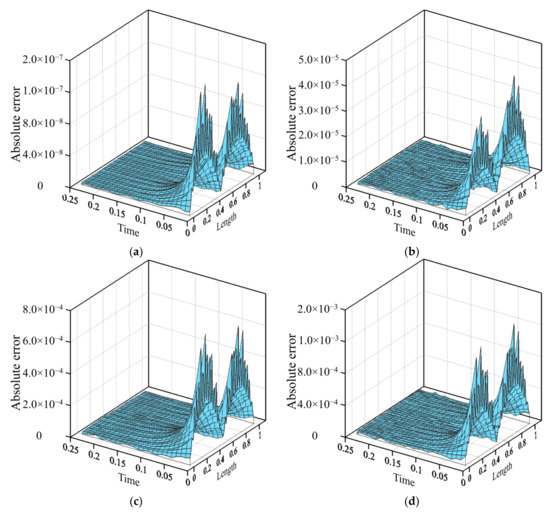
Figure 13.
Absolute error of the computed temperature: (a) e = 0, (b) e = 0.01, (c) e = 0.1, (d) e = 0.4.
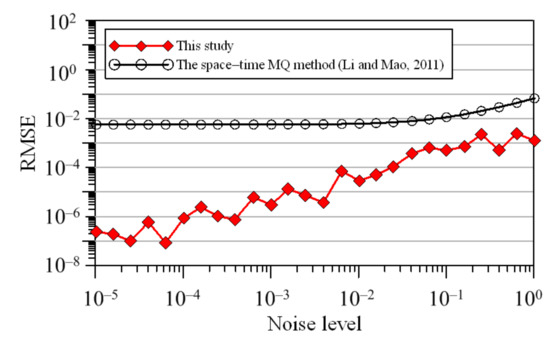
Figure 14.
The RMSE versus different noise levels.
5. Conclusions
In this article, we present the collocation method with a new space–time radial basis function for dealing with backward heat conduction problems. The innovative concepts of our method are addressed in detail. We conclude the findings as follows:
- In this article, the novel space–time radial polynomial basis function (SRPBF) is first proposed for the collocation method. Since the SRPBF is infinitely differentiable and the corresponding derivative is a smooth and nonsingular series function, the shape parameter is not required in the proposed method, which may mitigate the main issue in the conventional radial basis function collocation method for determining an optimal shape parameter.
- We propose a new idea for collocating the source points using the inner and outer source collocation schemes. Results demonstrate that the outer source collocation scheme may obtain more accurate results than the regular inner source collocation scheme. Furthermore, results indicate that the location of the source points outside the space–time domain may be not sensitive to the accuracy while the dilation parameter ranges from 2 to 7.
- Results of numerical examples demonstrate that our approach may obtain better solutions than those of the conventional radial basis function collocation method. Since all the collocation points are placed in the space–time domain, the one–dimensional heat conduction initial value problem is turned into the two–dimensional boundary value problem such that the heat conduction problem can be solved without utilizing the conventional time–marching techniques. It is found that the absolute error of our approach does not propagate with the simulation time. Additionally, our approach may yield better solutions than those of the radial basis function collocation method with the time–marching scheme.
- Numerical results demonstrate that the terms of the SRPBF may not be sensitive to the computed results. Furthermore, the absent heat data on the inaccessible boundary can be recovered with high accuracy even when severely ill–posed inverse backward heat conduction problems under large noises are considered.
Author Contributions
C.-Y.K. developed the conceptualization, and wrote the manuscript; C.-Y.L. worked on the mathematical development, performed the numerical analysis, and wrote the manuscript; J.-E.X. analyzed the data; M.-R.C. worked on the data curation. All authors have read and agreed to the published version of the manuscript.
Funding
This study carried out in 2019 to 2020 (MOST 108-2621-M-019-008) was supported by the Ministry of Science and Technology (MOST), Taiwan, the Republic of China.
Acknowledgments
The authors appreciate the MOST for providing financial support.
Conflicts of Interest
The authors declare no conflicts of interest.
References
- Li, M.; Monjiza, A.; Xu, Y.G.; Wen, P.H. Finite block Petrov–Galerkin method in transient heat conduction. Eng. Anal. Bound. Elem. 2015, 60, 106–114. [Google Scholar] [CrossRef]
- Gu, Y.; He, X.; Chen, W.; Zhang, C. Analysis of three-dimensional anisotropic heat conduction problems on thin domains using an advanced boundary element method. Comput. Math. Appl. 2018, 75, 33–44. [Google Scholar] [CrossRef]
- Grabski, J.K. Numerical solution of non-Newtonian fluid flow and heat transfer problems in ducts with sharp corners by the modified method of fundamental solutions and radial basis function collocation. Eng. Anal. Bound. Elem. 2019, 109, 143–152. [Google Scholar] [CrossRef]
- Li, M.; Jiang, T.; Hon, Y.C. A meshless method based on RBFs method for nonhomogeneous backward heat conduction problem. Eng. Anal. Bound. Elem. 2010, 34, 785–792. [Google Scholar] [CrossRef]
- Shigeta, T.; Young, D.L. Regularized solutions with a singular point for the inverse biharmonic boundary value problem by the method of fundamental solutions. Eng. Anal. Bound. Elem. 2011, 35, 883–894. [Google Scholar] [CrossRef]
- Zheng, H.; Zhang, C.; Wang, Y.; Chen, W.; Sladek, J.; Sladek, V. A local RBF collocation method for band structure computations of 2D solid/fluid and fluid/solid phononic crystals. Int. J. Numer. Methods Eng. 2017, 110, 467–500. [Google Scholar] [CrossRef]
- Jankowska, M.A.; Karageorghis, A.; Chen, C.S. Improved Kansa RBF method for the solution of nonlinear boundary value problems. Eng. Anal. Bound. Elem. 2018, 87, 173–183. [Google Scholar] [CrossRef]
- Hong, Y.; Lin, J.; Chen, W. Simulation of thermal field in mass concrete structures with cooling pipes by the localized radial basis function collocation method. Int. J. Heat Mass Transf. 2019, 129, 449–459. [Google Scholar] [CrossRef]
- Lin, Q.; Wang, J.; Hong, J.; Liu, Z.; Wang, Z. A biomimetic generative optimization design for conductive heat transfer based on element-free Galerkin method. Int. Commun. Heat Mass Transf. 2019, 100, 67–72. [Google Scholar] [CrossRef]
- Qiao, Y.; Zhai, S.; Feng, X. RBF-FD method for the high dimensional time fractional convection-diffusion equation. Int. Commun. Heat Mass Transf. 2017, 89, 230–240. [Google Scholar] [CrossRef]
- Li, N.; Su, H.; Gui, D.; Feng, X. Multiquadric RBF-FD method for the convection-dominated diffusion problems base on Shishkin nodes. Int. J. Heat Mass Transf. 2018, 118, 734–745. [Google Scholar] [CrossRef]
- Soleimani, S.; Jalaal, M.; Bararnia, H.; Ghasemi, E.; Ganji, D.D.; Mohammadi, F. Local RBF-DQ method for two-dimensional transient heat conduction problems. Int. Commun. Heat Mass Transf. 2010, 37, 1411–1418. [Google Scholar] [CrossRef]
- Islam, S.; Ismail, S. Meshless collocation procedures for time-dependent inverse heat problems. Int. J. Heat Mass Transf. 2017, 113, 1152–1167. [Google Scholar] [CrossRef]
- Ferreira, A.J.M.; Martins, P.A.L.S.; Roque, C.M.C. Solving time-dependent engineering problems with multiquadrics. J. Sound Vibr. 2005, 280, 595–610. [Google Scholar] [CrossRef]
- Zhu, F.; Yu, Z.; Zhao, L.; Xue, M.; Zhao, S. Adaptive-mesh method using RBF interpolation: A time-marching analysis of steady snow drifting on stepped flat roofs. J. Wind Eng. Ind. Aerodyn. 2017, 171, 1–11. [Google Scholar] [CrossRef]
- Ku, C.-Y.; Liu, C.-Y.; Yeih, W.; Liu, C.-S.; Fan, C.-M. A novel spacetime meshless method for solving backward heat conduction problem. Int. J. Heat Mass Transf. 2019, 130, 109–122. [Google Scholar] [CrossRef]
- Tezduyar, T.E.; Sathe, S.; Keedy, R.; Stein, K. Space–time finite element techniques for computation of fluid–structure interactions. Comput. Meth. Appl. Mech. Eng. 2006, 195, 2002–2027. [Google Scholar] [CrossRef]
- Yue, X.; Wang, F.; Hua, Q.; Qiu, X.Y. A novel space–time meshless method for nonhomogeneous convection–diffusion equations with variable coefficients. Appl. Math. Lett. 2019, 92, 144–150. [Google Scholar] [CrossRef]
- Ku, C.-Y.; Liu, C.-Y.; Xiao, J.-E.; Huang, W.-P.; Su, Y. A spacetime collocation Trefftz method for solving the inverse heat conduction problem. Adv. Mech. Eng. 2019, 11, 1–11. [Google Scholar] [CrossRef]
- Ku, C.Y.; Liu, C.Y.; Su, Y.; Yang, L.; Huang, W.P. Modeling tide–induced groundwater response in a coastal confined aquifer using the spacetime collocation approach. Appl. Sci. 2020, 10, 439. [Google Scholar] [CrossRef]
- Klaij, C.M.; van der Vegt, J.J.W.; van der Ven, H. Space–time discontinuous Galerkin method for the compressible Navier–Stokes equations. J. Comput. Phys. 2006, 217, 589–611. [Google Scholar] [CrossRef]
- Sudirham, J.J.; van der Vegt, J.J.W.; van Damme, R.M.J. Space–time discontinuous Galerkin method for advection–diffusion problems on time-dependent domains. Appl. Numer. Math. 2006, 56, 1491–1518. [Google Scholar] [CrossRef]
- Shojaei, A.; Mossaiby, F.; Zaccariotto, M.; Galvanetto, U. A local collocation method to construct Dirichlet-type absorbing boundary conditions for transient scalar wave propagation problems. Comput. Meth. Appl. Mech. Eng. 2019, 356, 629–651. [Google Scholar] [CrossRef]
- Mossaiby, F.; Shojaei, A.; Boroomand, B.; Zaccariotto, M.; Galvanetto, U. Local Dirichlet-type absorbing boundary conditions for transient elastic wave propagation problems. Comput. Meth. Appl. Mech. Eng. 2020, 362, 112856. [Google Scholar] [CrossRef]
- Boroomand, B.; Soghrati, S.; Movahedian, B. Exponential basis functions in solution of static and time harmonic elastic problems in a meshless style. Int. J. Numer. Methods Eng. 2010, 81, 971–1018. [Google Scholar] [CrossRef]
- Liu, C.-Y.; Ku, C.-Y.; Xiao, J.-E.; Yeih, W. A novel spacetime collocation meshless method for solving two-dimensional backward heat conduction problems. CMES 2019, 118, 229–252. [Google Scholar] [CrossRef]
- Li, Z.; Mao, X.Z. Global space–time multiquadric method for inverse heat conduction problem. Int. J. Numer. Methods Eng. 2011, 85, 355–379. [Google Scholar] [CrossRef]
- Hamaidi, M.; Naji, A.; Charafi, A. Space–time localized radial basis function collocation method for solving parabolic and hyperbolic equations. Eng. Anal. Bound. Elem. 2016, 67, 152–163. [Google Scholar] [CrossRef]
- Fasshauer, G.E.; Zhang, J.G. On choosing “optimal” shape parameters for RBF approximation. Numer. Algorithms 2007, 45, 345–368. [Google Scholar] [CrossRef]
- Scheuerer, M. An alternative procedure for selecting a good value for the parameter c in RBF-interpolation. Adv. Comput. Math. 2011, 34, 105–126. [Google Scholar] [CrossRef]
- Zhao, R.; Li, C.; Guo, X.; Fan, S.; Wang, Y.; Yang, C. A block iteration with parallelization method for the greedy selection in radial basis functions based mesh deformation. Appl. Sci. 2019, 9, 1141. [Google Scholar] [CrossRef]


© 2020 by the authors. Licensee MDPI, Basel, Switzerland. This article is an open access article distributed under the terms and conditions of the Creative Commons Attribution (CC BY) license (http://creativecommons.org/licenses/by/4.0/).