Abstract
Colonoscopy, which refers to the endoscopic examination of colon using a camera, is considered as the most effective method for diagnosis of colorectal cancer. Colonoscopy is performed by a medical doctor who visually inspects one’s colon to find protruding or cancerous polyps. In some situations, these polyps are difficult to find by the human eye, which may lead to a misdiagnosis. In recent years, deep learning has revolutionized the field of computer vision due to its exemplary performance. This study proposes a Convolutional Neural Network (CNN) architecture for classifying colonoscopy images as normal, adenomatous polyps, and adenocarcinoma. The main objective of this study is to aid medical practitioners in the correct diagnosis of colorectal cancer. Our proposed CNN architecture consists of 43 convolutional layers and one fully-connected layer. We trained and evaluated our proposed network architecture on the colonoscopy image dataset with 410 test subjects provided by Gachon University Hospital. Our experimental results showed an accuracy of 94.39% over 410 test subjects.
1. Introduction
The Gastrointestinal (GI) tract, or the digestive tract, is a system of organs responsible for digestion in humans. Like all other parts of the human body, the GI tract may have various diseases such as inflammatory diseases, autoimmune diseases, tumorous diseases, etc. To diagnose these diseases, clinical medical examination is required, which may include procedures like fecal occult blood test, endoscopy, etc. In general, colonoscopy is considered as the most accurate method for identifying lesions in one’s colon. In addition, colonoscopy is also used for therapeutic purposes. Colorectal cancer is the second leading cause of cancer deaths and is one of the five most important cancers to be screened. According to the National Statistical Office (NSO) survey in 2016, colorectal cancer was the third most common cause of lung cancer and liver cancer. In the past, the colorectal cancer incidence rate was high in Western countries. However, the incidence rate is rapidly increasing in South Korea as well. According to the adenoma-cancer continuum hypothesis, 95% of colorectal cancers occurring in the general population are advanced through the adenoma stage. Therefore, early detection and elimination of polyps during the adenoma stage are crucial in the prevention of colorectal cancer [1]. Colorectal cancer is diagnosed by a physician, and the authenticity of this diagnosis depends on the physician’s experience. Although certain objective criteria are used to ensure an accurate diagnosis, however, most physicians tend to follow a subjective criterion. Therefore, the results of an endoscopic colposcopy have a very subjective disadvantage [2]. The introduction of a system based on artificial intelligence can assist in obtaining a more accurate diagnosis and reduce human errors.
Attempts to analyze medical images using computerized methods date back many decades. The concept of Computer Aided Diagnosis (CAD) appeared in the 1970s when scanned medical images were analyzed on a computer. In the 1970s and 1990s, rule-based systems and expert systems were widely used. Rule-based systems use low-level image processing to extract edges and lines using filters. Mathematical structures are used to match circles and ellipses to obtain and analyze components. On the other hand, an expert system is evaluated as Good Old-Fashioned Artificial Intelligence (GOFAI) by analyzing the results of images using several conditional statements (if-else statements) [3].
Training data to improve the performance of a system were popularized in the late 1990s. This process required two main steps, namely feature extraction and classification. Features such as color, shape, texture, etc., are extracted during the feature extraction step. The most crucial step is to extract important features to represent the image. The extracted features are analyzed using various machine learning algorithms. The work done by [3,4,5,6,7] followed the same approach, which included feature extraction steps having several linear classifiers for classification. However, such methods rely on texture analysis, which requires expert knowledge about the features during the extraction process. Hence, they lack generalization and cannot be useful for transfer capabilities.
Currently, deep learning is widely used in medical image analysis. The 1998 paper by Yann LeCun [8] laid the foundation of today’s deep learning. Artificial intelligence using deep learning has shown excellent results in various fields such as speech recognition, language discrimination, behavior recognition, and image retrieval. Mostly medical image analysis deals with diagnosing diseases and detecting the affected area. Disease diagnosis using artificial intelligence is an active research area due to the development and state-of-the-art performance of deep learning. Recently, CNN has been reported to be highly useful in the field of endoscopy, especially Esophagogastroduodenoscopy (EGD), capsule endoscopy, and colonoscopy. The works done by [9,10,11,12] utilized a CNN-based diagnostic system to localize and classify EGD images effectively. Further, it was also applied to colonoscopy images to detect and classify colorectal polyps [13,14,15,16], and it was shown that the CNN-based method outperformed the traditional hand-crafted features method. Other typical usages of deep learning for disease diagnosis include skin cancer screening and diabetic retinopathy diagnosis [17,18]. Esteva [17] used Google’s Inception v3 [19] model to recognize 757 types of skin cancer. In addition, CNN was used to measure the severity of knee osteoarthritis in X-ray images and to detect lymph nodes in [20] and [21], respectively. CNN has also achieved good results in detecting brain tumors [22,23] and in lung nodule classification [24]. A better model and data are required to obtain good performance. Although the availability of a large amount of data has significantly increased performance, good quality training data are also needed to increase the diagnostic ability of the network. However, since medical images are obtained in a relatively controlled situation, they are stereotypical and can provide a good generalization performance even with a relatively small dataset. Furthermore, the number of layers in the network also plays a vital role to extract deep features from the images.
In this paper, we analyze the performance of the networks with the addition of different numbers of layers and propose a convolutional neural network that can classify normal colon, adenomatous polyp, and adenocarcinoma in colonoscopy images.
2. Image Classification Using Deep Learning
In the late 1990s, the LeNet [8] architecture was used for image classification using deep learning. LeNet’s architecture consists of a convolution layer, a pooling layer, and a fully-connected layer. The architecture of most deep image classification methods is inspired by LeNet. The operation performed in the convolution layer is given by Equation (1).
where refers to the ith pixel, corresponds to the weight value used for convolution, * denotes the convolution operation, and is the bias. The kernel W slides across the image and performs the convolution operation between and . The convolution output for all pixels of an image results in a feature map . Multiple kernels are used to generate multiple feature maps.
To reduce the image size, the pooling layer selects the maximum value in k-sized kernels at row r and column h in feature map F as shown in Equation (2). This procedure is known as max-pooling. If the average value is extracted instead of the maximum value, it is known as average pooling.
AlexNet [25], published in 2012, consists of five convolution and three fully-connected layers as shown in Figure 1. To solve the problem of the vanishing gradient, AlexNet replaces the existing sigmoid function or hyperbolic tangent activation function with the Rectified Linear Units (ReLU) [26] activation function as shown in Equation (3). To reduce overfitting, the dropout [27] method was applied for neural network learning. The AlexNet structure showed excellent results with a 15.4% test error rate in the image recognition part of ImageNet.
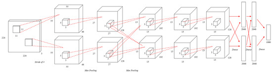
Figure 1.
An illustration of the architecture of AlexNet.
Two years after AlexNet was published, VGGNet [28] was developed by the University of Oxford. VGGNet consists of up to sixteen convolution layers. Unlike AlexNet, which uses a variety of kernel sizes, VGGNet reduces the number of parameters by using a fixed kernel size of 3 × 3. The nonlinearity in a network increases with the increase in the number of convolution layers. This aids in extracting more unique features.
A limitation with deep learning is that it may be trained poorly due to the slope loss as the architecture gets deeper. To solve this problem, ResNet [29] introduced the method of a block structure as shown in Figure 2 in which the input layer and the output layer are connected to each other. This structure is called the residual structure, and it is a structure that learns to minimize the difference between the input and output. Through this structure, the problem of slope disappearance is solved, and the training result is compared and evaluated by increasing the layers of the neural network.
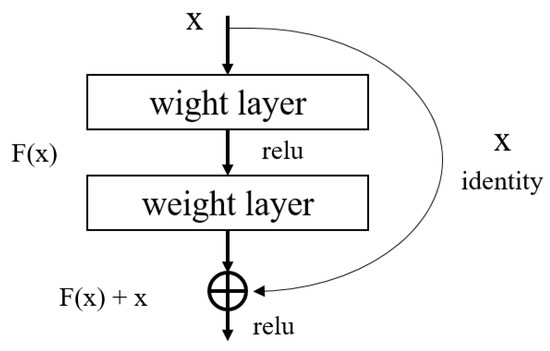
Figure 2.
Residual learning: a building block in ResNet.
Further, DenseNet [30] was introduced in 2017, where each layer takes all preceding feature maps as the input. Unlike ResNet, DenseNet has a structure in which an input layer and an output layer having the same feature map size are directly connected to each other and transmitted as the input values of the next layer as shown in Figure 3. It has small parameters and fewer computations with better performance than the state-of-the-art.
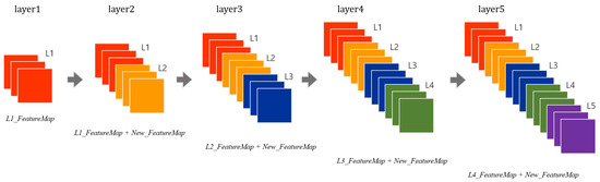
Figure 3.
A five-layer dense block in DenseNet.
3. Proposed Network Architecture
In this section, we propose and describe our convolutional neural network architecture for classification of colonoscopy images.
3.1. Structure
The proposed network architecture consists of a total of 43 convolution layers, five pooling layers, and a fully-connected layer as shown in Figure 4. The size of the input image is resized to 224 × 224 pixels. According to VGGNet [28], we used a three by three kernel for each of the convolution layers. The three by three kernel has the same effect as the use of 7 × 7 and 5 × 5 kernels. The dotted line in Figure 4 shows the functions performed between the preceding and the next convolution layer. After every convolution layer, batch normalization is applied, which is followed by the ReLU activation function. This structure was inspired by the ResNet [29] structure and is applied in the same way in this study. The feature map size reduction is performed five times in total. Max-pooling is performed by a 2 × 2 kernel in all pooling layers except the last pooling layer. In the last pooling layer, global average pooling is performed using a 7 × 7 kernel. Lastly, the fully connected layer consists of 1024 neurons, which are connected to the output layer composed of three classes.
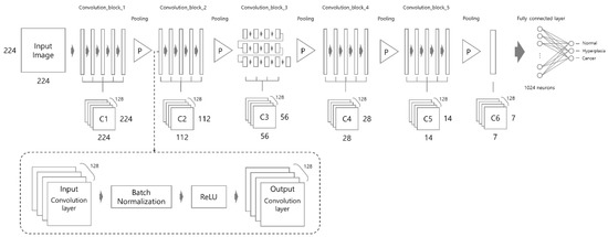
Figure 4.
Proposed network architecture. Note that each long rectangle means “convolution layer”.
3.2. Number of Convolution Layers
In this section, we discuss the influence of the number of convolution layers and discuss the proposed number of convolution layers. As shown in Figure 5, if we calculate a convolution product with a kernel size of three centered at , the result of the first convolution product is obtained by the influence of input values , , and . In the result of second convolution product, is the result from the convolution product of , , and of Hidden Layer 1. , , and are derived from , , , , and of the input layer. Therefore, is also affected by , , , , and of the input layer. In other words, the result is calculated by a kernel with the identical kernel size of the first convolution layer. However, the result of the convolution product shows the effect of it, which is a size twice as large asthe size of the kernel used in the first layer as shown by the blue area in Figure 5. In this way, when calculating the convolution product in Hidden Layer 2, is calculated by , , and with a kernel of size three, but indirectly, it is affected by the kernel of size seven in the first input layer. Therefore, the increase of the convolution layers can be expected to increase the size of the kernel. When applied to 2D images, if the number of convolution layers is increased, it can be expected to increase the size of the kernel.
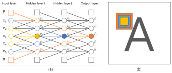
Figure 5.
Influence of the number of convolution layers. (a) Influence on neural networks; (b) influence on 2D images.
The successive convolution layers have different influences depending on the size of the image. As shown in Figure 6, convolutions with the first down sampling and second down sampling use the same size kernel, but the influence of the convolution product applied to each image size is different.
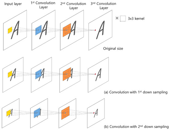
Figure 6.
Influence area of the convolution product according to the size of the 2D image.
4. Experiments
Our dataset consisted of three types of images, which were used for training and testing our network. Sample images from our dataset can be seen in Figure 7, where Figure 7a shows colonoscopy images of a normal person, Figure 7b shows colonoscopy images containing an adenomatous polyp, and Figure 7c shows colonoscopy images containing a cancerous adenomatous polyp. As shown in Figure 7, the colon of a normal person is without any polyps in the mucosa. When a polyp develops in the colon of a normal person (see Figure 7b), it can develop into a relatively large adenomatous polyp (see Figure 7c). Adenocarcinoma of the adenomatous polyps develops into malignant tumors and become cancer. The shape and size of the polyps developed by the cancer appear in various forms without any specific rules (see Figure 7c).
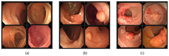
Figure 7.
Endoscopy image type in this experiment. (a) Normal images; (b) adenoma images; (c) adenocarcinoma images.
4.1. Experimental Data
Our original image dataset consisted of 449 cancer images, 626 adenomatous polyp images, and 773 normal images as shown in Table 1. However, this meager amount of data was insufficient for a deep neural network. To tackle this issue, we used data augmentation to increase the dataset size. Specifically, each image was rotated at various angles between 10° and 360°. After data augmentation, we obtained 16,609 adenocarcinoma images, 16,616 adenomatous polyposis images, and 16,233 normal images as shown in Table 1. Our final dataset consisted of a total of 49,458 endoscopic images. Our test dataset consisted of 140 cancer images, 142 adenomatous polyp images, and 128 normal images as shown in Table 2.

Table 1.
Configuration of our training dataset.
Table 2.
Configuration of our test dataset.
4.2. Experiments of Convolution Layer
As described above, the effect of the convolution differed according to the number of convolutions and the pooling phase. In this paper, In order to find an optimal model for colon endoscopy recognition, we performed experiments in which the convolution layer structure changed as shown in Table 3. We proposed the number of layers that had the highest result by changing the number of the convolutional layers after each pooling step. In the first experiment of the convolution layers, we experimented to increase the number of convolution layers by 4, 6, and 8 configurations, which were the same numbers of convolution layers after each pooling step. The second experiment of the convolution layers was an experiment in which the number of convolution layers was increased around a specific pooling step.
Table 3.
Configuration of the experiment of the convolution layers.
As a result of the first experiment, the accuracy was gradually increased with the increasing number of convolution layers as shown in Table 4. This showed that the result was better as the number of convolution layers increased, but when the number of convolution layers was further increased, the performance deteriorated due to over-fitting. In a second experiment in which the convolution layers were increased around a particular scale, high accuracy was demonstrated when the largest number of convolution layers was constructed after the second pooling step.
Table 4.
The result of the experiment of the convolution layers.
4.3. Experimental Evaluation
This section shows various metrics used for evaluation during the experiments on the testing sets. If a model correctly predicted the positive class, then it is known as a True Positive (TP). Similarly, if a model predicts the negative class correctly, then it is known as a True Negative (TN). On the other hand, if a model incorrectly predicts a positive class, then it is referred to as a False Positive (FP). A False Negative (FN) is when the model incorrectly predicts the negative class. The accuracy, precision, and sensitivity are calculated using Equation (4).
4.4. Network Training
The implementation was based on Keras with a TensorFlow backend. We used stochastic gradient descent with a batch size of 8 for all methods. The learning rate started from 0.001 and decreased by a factor of 0.1 when the tolerance level exceeded 4. We used a weight decay of 0.0001 and a momentum of 0.9 without an accelerated gradient. Overall training was done for different network architectures on a single NVIDIA GTX 1080 Ti GPU. We fine-tuned DenseNet-121, ResNet-152, and VGG16 using RMSProp [31] with a decay of 0.9. Each network was trained for 100 epochs. Figure 8 shows the inference time during training each architecture with same number of batches. As can be seen in the figure, the proposed method processed fewer images, but it had fewer parameters in comparison to other architectures. Due to the increasing number of channels added in the existing CNNs, its complexity overfit the model. However, we used the same number of channels in all layers and increased the convolutional layer, which made the method less complex. Table 5 shows the overview of each network’s computation capability with its parameters.
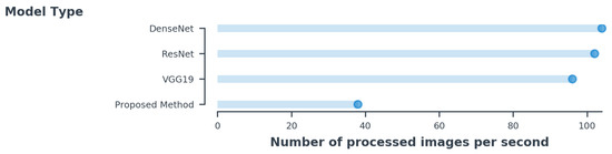
Figure 8.
The inference time per image is estimated for the same batch size of 8 for all methods.
Table 5.
Network complexities with the parameters.
4.5. Performance Evaluation
In this section, we compare the performance of the proposed method with the existing CNN method due to the limited work on colorectal diseases using deep learning. We first evaluated different layers of the CNN as shown in Table 4. Next, we evaluated the proposed method with the baseline architectures with the same number of parameters. The results of our experimentation and evaluation are summarized in Table 6, Table 7, Table 8 and Table 9. Table 9 shows the confusion matrix results for the test data, whereas Table 6 shows the sensitivity, precision, and accuracy of the test results.
Table 6.
Confusion matrix of the experimental results.
Table 7.
Error images.
Table 8.
Experimental results.
Table 9.
Accuracy with other CNN networks.
In the experimental results with 128 normal images, there were 8 TN cases, which showed food and excrement in colonic mucosa and colorectal crescentic wrinkles similar to polyps. Further, it was also observable that the problem that had the biggest impact on the overall error rate was images with small-sized polyps that were difficult to detect in the normal area. It showed a 4.6% error rate in the experimental results. This was the most error of the total error rate of 5.61%. In all the test data, adenoma images showed the lowest precision by 91.21%, but adenocarcinoma images showed the highest accuracy of 97.05%. The accuracy of the whole image was 94.39%.
The comparison with the well-known network in the ImageNet Challenge is shown in Table 9. The test result showed 87% on VGG19 [28], 90% on ResNet [29], and 89% on DenseNet [30] when trained with the same dataset.
5. Discussion
In this work, we presented an automated system to classify colorectal diseases with high accuracy. The experimental evaluation showed that the proposed method could accurately differentiate high-risk polyps and adenocarcinoma effectively in the endoscopic domain. This method leveraged the VGG architecture and enabled the development of effective models with high accuracy for colorectal images in comparison to existing approaches. Although this best-performing model processed fewer images per second during inference, it was more important to classify the diseases more accurately. The availability of fewer data in the medical domain made it difficult for the CNN model to converge. However, our proposed method had much fewer parameters and converged fast when the dataset had fewer images. This technology will improve the quality of colorectal cancer screening and performance if combined with endoscopic experts.
One drawback of our method for endoscopic characterization was the black box approach to the results. Therefore, the visualization method in the network after or during training needs to be developed for improvement. It will surely help doctors or medical experts to gain insight into the influential regions and features in the image. Beside this, we plan to compare our performance with medical experts and validate the efficacy of the method in clinical practice.
6. Conclusions
In this paper, we used our proposed deep neural network architecture to recognize normal, adenomatous polyps, and adenocarcinoma in colonoscopy images. We studied the effect of the addition of convolutional layers in the network, and based on this, we proposed a convolutional neural network architecture that consisted of a total of 43 convolutions and one fully-connected layer. To evaluate our network, we calculated the sensitivity, precision, and accuracy. With extensive experiments and evaluation, it was proven that our method was more accurate and able to extract features from the colorectal images. In the future, the endoscopy diagnosis system will be developed and improved.
7. Data Availability
The endoscopy image data used to support the findings of this study were supplied by Yoon-Jae Kim under license and so cannot be made freely available. Requests for access to these data should be made to yoonmed@gilhospital.com.
Author Contributions
Conceptualization, S.-W.L. and Y.-J.K.; methodology, H.-C.P. and S.-W.L.; software, H.-C.P.; validation, H.-C.P.; formal analysis, H.-C.P. and S.-W.L.; investigation, H.-C.P.; data curation, H.-C.P.; writing–original draft preparation, H.-C.P.; writing–review and editing, H.-C.P.; visualization, H.-C.P.; supervision, S.-W.L.; project administration, Y.-J.K. All authors have read and agreed to the published version of the manuscript.
Funding
This work was supported by the research fund of Gil Medical University (2017-06) and the GRRCprogram of Gyeonggi province (GRRC-Gachon2017(B01), Analysis of behavior based on senior life log).
Conflicts of Interest
The authors declare that there are no conflicts of interest regarding the publication of this paper.
References
- Watson, J.D.; Crick, F. A structure for deoxyribose nucleic acid. Nature 1953, 171, 737–738. [Google Scholar] [CrossRef]
- Hixson, L.; Fennerty, M.B.; Sampliner, R.; McGee, D.; Garewal, H. Prospective study of the frequency and size distribution of polyps missed by colonoscopy. J. Natl. Cancer Inst. 1990, 82, 1769–1772. [Google Scholar] [CrossRef]
- Litjens, G.; Kooi, T.; Bejnordi, B.E.; Setio, A.A.A.; Ciompi, F.; Ghafoorian, M.; Van Der Laak, J.A.; Van Ginneken, B.; Sánchez, C.I. A survey on deep learning in medical image analysis. Med. Image Anal. 2017, 42, 60–88. [Google Scholar] [CrossRef] [PubMed]
- Häfner, M.; Tamaki, T.; Tanaka, S.; Uhl, A.; Wimmer, G.; Yoshida, S. Local fractal dimension based approaches for colonic polyp classification. Med. Image Anal. 2015, 26, 92–107. [Google Scholar] [CrossRef] [PubMed]
- Wimmer, G.; Tamaki, T.; Tischendorf, J.J.; Häfner, M.; Yoshida, S.; Tanaka, S.; Uhl, A. Directional wavelet based features for colonic polyp classification. Med. Image Anal. 2016, 31, 16–36. [Google Scholar] [CrossRef]
- Tamaki, T.; Yoshimuta, J.; Kawakami, M.; Raytchev, B.; Kaneda, K.; Yoshida, S.; Takemura, Y.; Onji, K.; Miyaki, R.; Tanaka, S. Computer-aided colorectal tumor classification in NBI endoscopy using local features. Med. Image Anal. 2013, 17, 78–100. [Google Scholar] [CrossRef] [PubMed]
- Stehle, T.; Auer, R.; Gross, S.; Behrens, A.; Wulff, J.; Aach, T.; Winograd, R.; Trautwein, C.; Tischendorf, J. Classification of colon polyps in NBI endoscopy using vascularization features. In Medical Imaging 2009: Computer-Aided Diagnosis; International Society for Optics and Photonics: Bellingham, WA, USA, 2009; Volume 7260, p. 72602S. [Google Scholar]
- LeCun, Y.; Bottou, L.; Bengio, Y.; Haffner, P. Gradient-based learning applied to document recognition. Proc. IEEE 1998, 86, 2278–2324. [Google Scholar] [CrossRef]
- Takiyama, H.; Ozawa, T.; Ishihara, S.; Fujishiro, M.; Shichijo, S.; Nomura, S.; Miura, M.; Tada, T. Automatic anatomical classification of esophagogastroduodenoscopy images using deep convolutional neural networks. Sci. Rep. 2018, 8, 7497. [Google Scholar] [CrossRef] [PubMed]
- Itoh, T.; Kawahira, H.; Nakashima, H.; Yata, N. Deep learning analyzes Helicobacter pylori infection by upper gastrointestinal endoscopy images. Endosc. Int. Open 2018, 6, E139–E144. [Google Scholar] [CrossRef]
- Shichijo, S.; Nomura, S.; Aoyama, K.; Nishikawa, Y.; Miura, M.; Shinagawa, T.; Takiyama, H.; Tanimoto, T.; Ishihara, S.; Matsuo, K.; et al. Application of convolutional neural networks in the diagnosis of Helicobacter pylori infection based on endoscopic images. EBioMedicine 2017, 25, 106–111. [Google Scholar] [CrossRef]
- Hirasawa, T.; Aoyama, K.; Tanimoto, T.; Ishihara, S.; Shichijo, S.; Ozawa, T.; Ohnishi, T.; Fujishiro, M.; Matsuo, K.; Fujisaki, J.; et al. Application of artificial intelligence using a convolutional neural network for detecting gastric cancer in endoscopic images. Gastric Cancer 2018, 21, 653–660. [Google Scholar] [CrossRef] [PubMed]
- Komeda, Y.; Handa, H.; Watanabe, T.; Nomura, T.; Kitahashi, M.; Sakurai, T.; Okamoto, A.; Minami, T.; Kono, M.; Arizumi, T.; et al. Computer-aided diagnosis based on convolutional neural network system for colorectal polyp classification: Preliminary experience. Oncology 2017, 93, 30–34. [Google Scholar] [CrossRef] [PubMed]
- Byrne, M.F.; Chapados, N.; Soudan, F.; Oertel, C.; Pérez, M.L.; Kelly, R.; Iqbal, N.; Chandelier, F.; Rex, D.K. Real-time differentiation of adenomatous and hyperplastic diminutive colorectal polyps during analysis of unaltered videos of standard colonoscopy using a deep learning model. Gut 2019, 68, 94–100. [Google Scholar] [CrossRef] [PubMed]
- Zhang, R.; Zheng, Y.; Mak, T.W.C.; Yu, R.; Wong, S.H.; Lau, J.Y.; Poon, C.C. Automatic detection and classification of colorectal polyps by transferring low-level CNN features from nonmedical domain. IEEE J. Biomed. Health Inform. 2016, 21, 41–47. [Google Scholar] [CrossRef]
- Yu, L.; Chen, H.; Dou, Q.; Qin, J.; Heng, P.A. Integrating online and offline three-dimensional deep learning for automated polyp detection in colonoscopy videos. IEEE J. Biomed. Health Inform. 2016, 21, 65–75. [Google Scholar] [CrossRef]
- Esteva, A.; Kuprel, B.; Novoa, R.A.; Ko, J.; Swetter, S.M.; Blau, H.M.; Thrun, S. Dermatologist-level classification of skin cancer with deep neural networks. Nature 2017, 542, 115. [Google Scholar] [CrossRef]
- Gulshan, V.; Peng, L.; Coram, M.; Stumpe, M.C.; Wu, D.; Narayanaswamy, A.; Venugopalan, S.; Widner, K.; Madams, T.; Cuadros, J.; et al. Development and validation of a deep learning algorithm for detection of diabetic retinopathy in retinal fundus photographs. JAMA 2016, 316, 2402–2410. [Google Scholar] [CrossRef]
- Szegedy, C.; Vanhoucke, V.; Ioffe, S.; Shlens, J.; Wojna, Z. Rethinking the inception architecture for computer vision. In Proceedings of the IEEE Conference on Computer Vision and Pattern Recognition, Las Vegas, NV, USA, 27–30 June 2016; pp. 2818–2826. [Google Scholar]
- Antony, J.; McGuinness, K.; O’Connor, N.E.; Moran, K. Quantifying radiographic knee osteoarthritis severity using deep convolutional neural networks. In Proceedings of the 2016 23rd International Conference on Pattern Recognition (ICPR), Cancún, Mexico, 4–8 December 2016; pp. 1195–1200. [Google Scholar]
- Roth, H.R.; Lu, L.; Seff, A.; Cherry, K.M.; Hoffman, J.; Wang, S.; Liu, J.; Turkbey, E.; Summers, R.M. A new 2.5 D representation for lymph node detection using random sets of deep convolutional neural network observations. In Proceedings of the International Conference on Medical Image Computing and Computer-Assisted Intervention, Boston, MA, USA, 14–18 September 2014; Springer: Cham, Switzerland, 2014; pp. 520–527. [Google Scholar]
- Havaei, M.; Davy, A.; Warde-Farley, D.; Biard, A.; Courville, A.; Bengio, Y.; Pal, C.; Jodoin, P.M.; Larochelle, H. Brain tumor segmentation with deep neural networks. Med. Image Anal. 2017, 35, 18–31. [Google Scholar] [CrossRef]
- Pereira, S.; Pinto, A.; Alves, V.; Silva, C.A. Brain tumor segmentation using convolutional neural networks in MRI images. IEEE Trans. Med Imaging 2016, 35, 1240–1251. [Google Scholar] [CrossRef]
- Shen, W.; Zhou, M.; Yang, F.; Yang, C.; Tian, J. Multi-scale convolutional neural networks for lung nodule classification. In Proceedings of the International Conference on Information Processing in Medical Imaging, Isle of Skye, UK, 28 June–3 July 2015; Springer: Cham, Switzerland, 2015; pp. 588–599. [Google Scholar]
- Krizhevsky, A.; Sutskever, I.; Hinton, G.E. Imagenet classification with deep convolutional neural networks. In Proceedings of the Advances in Neural Information Processing Systems, Lake Tahoe, NV, USA, 3–6 December 2012; pp. 1097–1105. [Google Scholar]
- Nair, V.; Hinton, G.E. Rectified linear units improve restricted boltzmann machines. In Proceedings of the 27th International Conference on Machine Learning (ICML-10), Haifa, Israel, 21–24 June 2010; pp. 807–814. [Google Scholar]
- Srivastava, N.; Hinton, G.; Krizhevsky, A.; Sutskever, I.; Salakhutdinov, R. Dropout: A simple way to prevent neural networks from overfitting. J. Mach. Learn. Res. 2014, 15, 1929–1958. [Google Scholar]
- Simonyan, K.; Zisserman, A. Very deep convolutional networks for large-scale image recognition. arXiv 2014, arXiv:1409.1556. [Google Scholar]
- He, K.; Zhang, X.; Ren, S.; Sun, J. Deep residual learning for image recognition. In Proceedings of the IEEE Conference on Computer Vision and Pattern Recognition, Las Vegas, NV, USA, 27–30 June 2016; pp. 770–778. [Google Scholar]
- Huang, G.; Liu, Z.; Van Der Maaten, L.; Weinberger, K.Q. Densely connected convolutional networks. In Proceedings of the IEEE Conference on Computer Vision and Pattern Recognition, Honolulu, HI, USA, 21–26 July 2017; pp. 4700–4708. [Google Scholar]
- Tieleman, T.; Hinton, G. Lecture 6.5-rmsprop: Divide the gradient by a running average of its recent magnitude. COURSERA Neural Netw. Mach. Learn. 2012, 4, 26–31. [Google Scholar]


© 2020 by the authors. Licensee MDPI, Basel, Switzerland. This article is an open access article distributed under the terms and conditions of the Creative Commons Attribution (CC BY) license (http://creativecommons.org/licenses/by/4.0/).