Unsteady Aerodynamic Characteristics Simulations of Rotor Airfoil under Oscillating Freestream Velocity

Abstract

The dynamic stall characteristics of rotor airfoil are researched by employing unsteady Reynolds-Averaged Navier-Stokes (RANS) method under oscillating freestream velocity conditions. In order to simulate the oscillating freestream velocity of airfoil under dynamic stall conditions, the moving-embedded grid method is employed to simulate the oscillating velocity. By comparing the simulated dynamic stall characteristics of two-dimensional airfoil and three-dimensional rotor, it is indicated that the dynamic stall characteristics of airfoil under oscillating freestream velocity reflect the actual dynamic stall characteristics of rotor airfoil in forward flight more accurately. By comparing the simulated results of OA209 airfoil under coupled freestream velocity/pitching oscillation conditions, it is indicated that the dynamic stall characteristics of airfoil associate with the critical value of Cp peaks (i.e., the dynamic stall characteristics of OA209 airfoil would be enhanced when the maximum negative pressure is larger than −1.08, and suppressed when this value is smaller than −1.08). By comparing the characteristics of vortices under different oscillating velocities, it indicates that the dissipation rate of leading edge vortex presents as exponent characteristics, and it is not sensitive to different oscillating velocities.

1. Introduction

In forward flight conditions, the freestream velocity of a helicopter rotor blade in the advancing side is larger than that of the retreating side due to the effect of forward flight. As a result, the inflow velocity of rotor airfoil varies with the rotor azimuth. Therefore, investigations on unsteady aerodynamic characteristics of rotor airfoil under oscillating freestream velocity are important, especially for the dynamic stall phenomenon [1,2]. To discover the physical essence of a rotor airfoil dynamic stall, a lot of research under steady freestream velocity (SFV) conditions has been accomplished by using the experimental method [3,4,5,6], theoretical method [7,8,9,10,11,12], and numerical method [13,14,15]. Hence, the dynamic stall of airfoil under SFV conditions is well-studied at present. However, the dynamic stall of rotor airfoil under oscillating freestream velocity (OFV) conditions was seldom taken into account in early researches.

In order to discover the physical phenomenon of dynamic stall under OFV condition, Favier [16] preliminarily researched dynamic stall characteristics of the NACA0012 under the condition of oscillating velocity by using the experimental method. After that, the aerodynamic loads of the NACA0012 airfoil were measured by Gursul [17,18] at a fixed angle of attack (AoA) under unsteady freestream conditions in a vertical unsteady water tunnel with a cross-sectional area of 45.7 × 45.7 cm. Based on this experiment, it was found that the lift coefficient (C_l) can be one order of magnitude higher under OFV conditions than that under SFV conditions. Gharali [19] investigated the dynamic stall of NACA0012 airfoil under variational velocity by employing the ANSYS Fluent software, and the results were indicated that the leading edge vortex (LEV) formation could be obviously affected by the phase angle between the oscillating pitch and the oscillating freestream velocity. However, the maximum AoA and maximum velocity of airfoil were superimposed in this research, which is much different from the actual working environment of a helicopter rotor in forward flight. As a result, the conclusions of the dynamic stall characteristics of two-dimensional (2D) airfoil may not coincide with that of a helicopter rotor airfoil. At the same time, a new experiment [20,21] was performed by the researchers of Ohio State University (OSU) to test the dynamic stall characteristics of SSC-A09 airfoil under oscillating velocity conditions. By comparing the measured C_l and C_m (pitching moment coefficient) under OFV conditions and SFV conditions, it was found that the lift curve slope and stall angle increased under the OFV conditions. However, due to the restriction of the experimental equipment, the maximum oscillating velocity (0.08 Ma) was much smaller than the normal forward flight velocity of the helicopter (Mach number of 0.1–0.3). Moreover, the aspect ratio of the blade model used in these experiments was only 1.0, which would generate obvious three-dimensional (3D) effects, and the characteristics of dynamic stall vortices would be influenced seriously. What is more, the added-mass effect due to the velocity variation would also influence the measured results in this research as mentioned in another study [22].

At the same time, Jones et al. [23,24,25] researched the dynamic stall characteristics of an airfoil under OFV conditions in horizontal free-surface water tunnel of the U.S. Air Force Research Laboratory. However, these studies were focused on aerodynamic characteristics of airfoil at fixed AoAs, which was much different from the working environment of a helicopter rotor. Meanwhile, the freestream velocities were also smaller than the rotational velocity of the helicopter rotor due to the restriction of water tunnel. Therefore, the dynamic stall characteristics of the rotor airfoil under the real environment of helicopter are still not included in these studies, and this issue is valuable to research more deeply.

As mentioned above, the dynamic stall characteristics of rotor airfoil under an actual working environment of a helicopter are not well studied. Previous research seldom focused on the characteristics of a dynamic stall vortex under coupled freestream velocity/pitching oscillation conditions directly. Therefore, the purpose of this study is to explore the effects of OFV on dynamic stall characteristics of rotor airfoil. In this research, the moving-embedded grid method [26,27] is adopted to simulate the oscillating velocity and pitching of an airfoil. The unsteady RANS equations coupling with third-order Roe-MUSCL spatial discretization scheme are chosen as the governing equations to predict the unsteady flowfield of an airfoil, and the highly-efficient implicit scheme of lower-upper symmetric Gauss–Seidel (LU-SGS) is adopted for temporal discretization. To capture the separated airflow and vortex more accurately, the SST $\mathrm{k}-\omega$ turbulence model is employed in the Computational Fluid Dynamics (CFD) code. Based on these methods, the dynamic stall characteristics of airfoil are researched under coupled conditions. It is indicated from the simulated results that the dynamic stall characteristics of airfoil associate with a critical value of Cp peak. By studying the vortices characteristics, it is illustrated that the dissipation rate of the LEV presents as exponent characteristics. However, this dissipation rate is not sensitive to oscillating velocity.

2. Aerodynamic Environment of Helicopter Rotor

The Figure 1a illustrates the velocity distribution of a helicopter rotor with blade tip, Mach number of 0.6, and advance ratio of 0.3. It is indicated that the rotor blade velocity varies with the rotor azimuth in forward flight. As a result, the relative freestream velocity of airfoil at different spanwise sections of rotor blade could be expressed as

$$Ma=M_B+M_F\sin \left(\omega t\right)$$

(1)

where, $M_B$ represents the rotational velocity of the blade, $M_F$ denotes the forward flight velocity of the helicopter, $\omega$ and $t$ represent the angular velocity and time, respectively.

Aiming at illustrating the relationship between the basic freestream velocity and the oscillating velocity, a normalized oscillating velocity $\lambda$ is defined as

$$\lambda =\frac{M_F}{M_B}$$

(2)

The AoA variation induced by cyclic pitching of the rotor blade can be written as

$$\alpha ={\alpha }_m+\mathsf{\Delta }\alpha \sin \left(\omega t+\pi \right)$$

(3)

where, ${\alpha }_m$ and $\mathsf{\Delta }\alpha$ represent the mean AoA and amplitude of pitch oscillation, respectively. In this environment, the variations of AoA (${\alpha }_m={8.0}^{°}$ and $\mathsf{\Delta }\alpha ={6.0}^{°}$) and freestream Mach number (M_B = 0.4 and M_F = 0.18) are shown in Figure 1b.

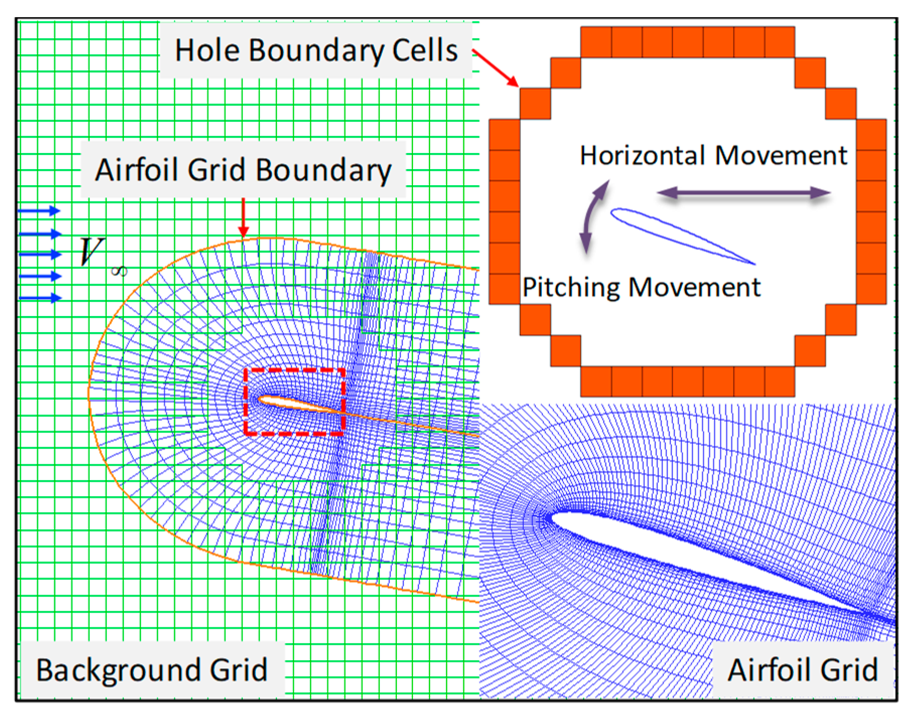
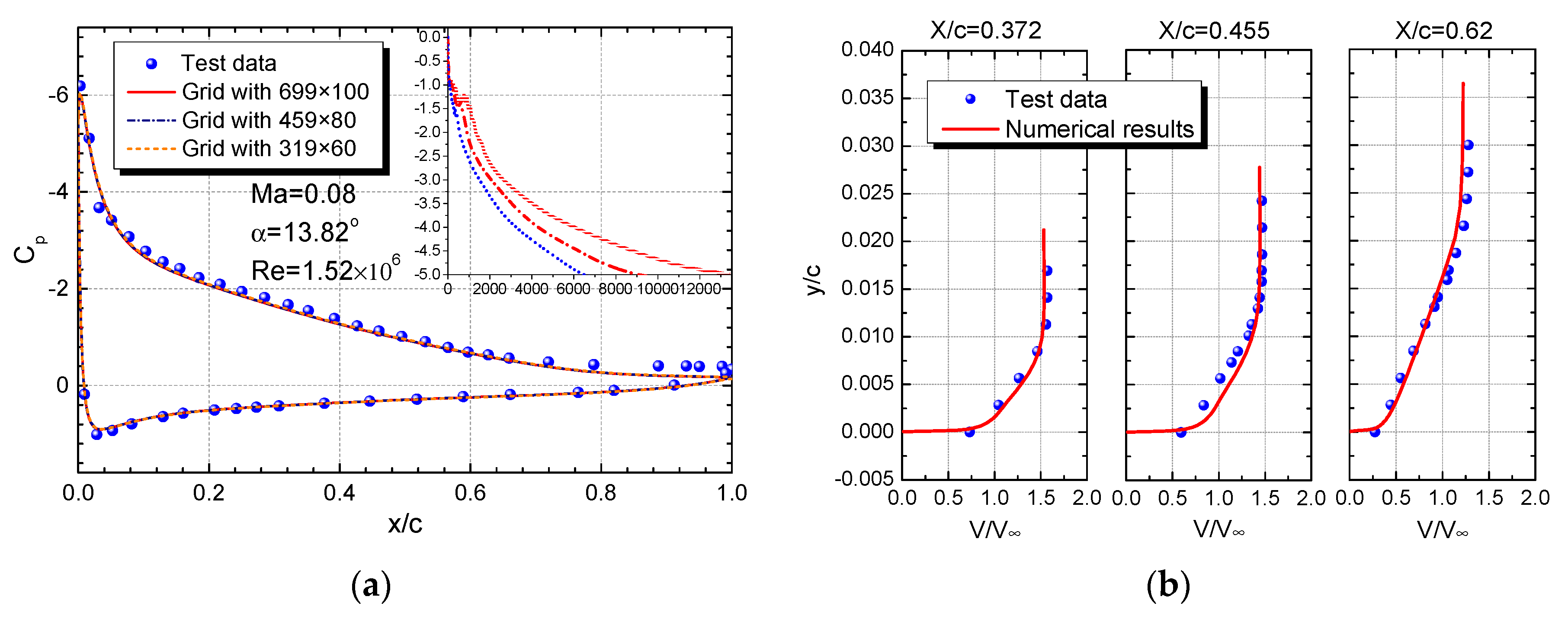
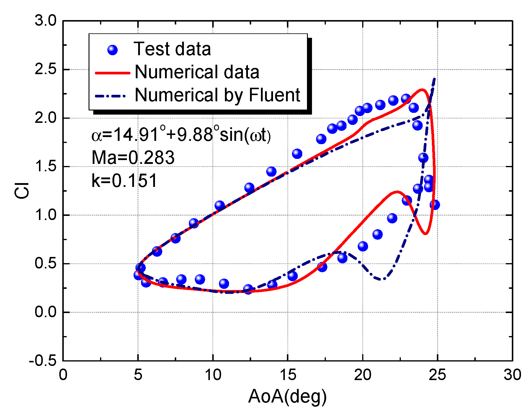
3. Numerical Simulation Method

In order to generate the computational grids around the OA209 airfoil, the Poisson equations [28] are chosen as the governing equations under 2D conditions. By solving these equations, the C-topology grids with 459 × 80 points are generated. To satisfy the requirement of OFV simulation, the far-field boundary of airfoil grids is fixed at 25 times the airfoil chord, and the y⁺ of the grids near the wall surface is smaller than 1.2. In this research, the background grid is composed of 300 × 300 points with a far-field boundary of 50 c (airfoil chord), and the inverse map method [29] is employed in this code to search donor element. As shown in Figure 2, the oscillating velocity is simulated by moving the airfoil back and forth periodically [30,31].

In order to simulate the unsteady compressible flowfield around an airfoil, the integral form of the Navier–Stokes equations is employed in this work, i.e.,

$$\frac{\partial }{\partial t}{\displaystyle \underset{\mathsf{\Omega }}{\iiint }Wd\mathsf{\Omega }}+{\displaystyle \underset{\partial \mathsf{\Omega }}{\iint }(F_c}-F_v)dS=0$$

(4)

where $W$ represents the conserved variables, $F_c$ and $F_v$ denote convective fluxes and viscous fluxes, respectively, i.e.,

$$W=\left[\begin{array}{l}\rho \\ \rho u\\ \rho v\\ \rho E\end{array}\right],F_c=\left[\begin{array}{l}\rho V_r\\ \rho u{V}_r+n_{x}p\\ \rho v{V}_r+n_{y}p\\ \rho H{V}_r+V_{t}p\end{array}\right],F_v=\left[\begin{array}{c}0\\ n_x{\tau }_{xx}+n_y{\tau }_{xy}\\ n_x{\tau }_{yx}+n_y{\tau }_{yy}\\ n_x{\mathsf{\Theta }}_x+n_y{\mathsf{\Theta }}_y\end{array}\right]$$

(5)

where $V_r=V-V_t$, $V$ is absolute velocity, $V_t$ is contravariant velocity. ${\tau }_{ij}$ denotes the viscous stresses, and ${\mathsf{\Theta }}_i$ is the term describing the heat condition in the fluid.

Meanwhile, the unsteady condition simulation is accomplished by employing the dual time-stepping approach. Then Equation (4) would be changed as

$$\frac{d({\mathsf{\Omega }}^{n+1}{W}^{\ast })}{d\tau }+R^{\ast }(W^{\ast })=0$$

(6)

where $W^{\ast }$ is the approximation for $W^{n+1}$, $\tau$ represents a pseudo time variable, and the unsteady residual is defined as

$$R^{\ast }(W^{\ast })=\frac{3W^{\ast }-4W^n+W^{n-1}}{2\mathsf{\Delta }t}+R(W^{\ast })$$

(7)

To improve the computational efficiency, the implicit LU-SGS [32,33] scheme is employed in this work. The two equation SST $\mathrm{k}-\omega$ turbulence model is employed to simulate the viscous stresses of the flowfield.

In order to verify the accuracy of the present grid system and flowfield solver, a case of the NACA4412 airfoil is presented in this section. In this case, the pressure coefficient (Cp) simulated by the present CFD method compared with the test data [34] is shown in Figure 3a. In this case, three different grids (699 × 100, 459 × 80, 319 × 60) are used to analyze the grid sensitivity. By comparing with the test data, it illustrated that the Cp simulated by the CFD method correlates well with test data for a different grid. However, the convergence of a larger grid is lower than coarse grid, but it still converges at least five orders of magnitude. It is indicated that the grid used in this research could satisfy the calculation requirement. Meanwhile, it is illustrated in Figure 3b that the velocity profiles are also close to the test data. As a result, it is indicated that the grid used in this research is suitable.

In order to verify the accuracy of the present CFD method used in the dynamic stall characteristic simulations of rotor airfoil, a typical case of dynamic stall about the NACA0012 airfoil is presented under the SFV condition in this section. The freestream Mach number is 0.283, the variation of AoA is $\alpha ={14.91}^{°}+{9.88}^{°}\sin (\omega t)$, and the reduced frequency (k) is 0.151. As shown in Figure 4, it is indicated that the simulated C_l by the present CFD method is correlated well with the test data of National Aeronautics and Space Administration (NASA) [35]. Meanwhile, the calculated results of the present CFD method are better than that calculated by Fluent software with SST $\mathrm{k}-\omega$ turbulence model.

Since we lack appropriate test data of rotor airfoil under dynamic stall conditions coupled with variational velocity, the theory of Isaacs [36] is employed to verify the accuracy of the present CFD method under OFV condition, as shown in Figure 5. It is illustrated that the numerical results correlate well with the theoretical data at $\lambda =0.4$, and the numerical results with $\lambda =0.8$ are basically close to the theoretical value. The deviation of the C_l/C_l0 at $\lambda =0.8$ could be attributed to the fact that the airflow compressibility and viscidity are neglected in the Isaacs theory, where C_l0 represents the lift force at steady freestream velocity. Consequently, it is indicated that the present CFD method is suitable for simulating unsteady characteristics of a rotor airfoil under dynamic stall conditions coupled with oscillating freestream velocity.

4. Analyses and Discussions

4.1. The Dynamic Stall Characteristics of Airfoil Under 3D Conditions

Aiming at researching the dynamic stall characteristics of rotor airfoil with OFV under actual rotor working conditions, a two-blade untwisted rotor model with a rectangular planform is designed based on the OA209 airfoil, and the aspect ratio of the rotor blade is 15.0. The blade grids with 356 × 70 × 90 points are generated based on the 2D airfoil grids, and the background grids are 176 × 99 × 156. The numerical simulation is performed at an advance ratio of 0.3 with blade tip, Mach number of 0.6, and the pitch angle is $\alpha ={10.0}^{°}-{6.0}^{°}\sin (\omega t)$. In this case, two different spanwise sections of blade, 0.6 R and 0.7 R (R is the radius of rotor), are selected to compare the numerical results under the 2D conditions, where the steady Mach numbers are 0.36 and 0.42, the unsteady Mach numbers are verified based on the steady Mach number with $\lambda$ of 0.5 and 0.43, respectively. The corresponding airflow information of different spanwise sections is shown in

Table 1. Airflow information at different blade sections.

Blade Section	${\mathit{M}}_{\mathit{B}}$	$\mathit{\lambda }$	k
0.6 R	0.36	0.5	0.0556
0.7 R	0.42	0.43	0.0476

.

In order to verify the accuracy of the present CFD method used in the 3D rotor condition, a case of SA349/2 rotor with an advance ratio of 0.26 is present in this section, just as shown in Figure 6 and Figure 7. The comparisons of normal force (Cn) and Cp distributions (0.75 r/R) are correlated well with the test data [37]. It is illustrated that the present CFD method can effectively simulate the unsteady aerodynamic characteristics of a rotor.

The comparisons of dynamic stall characteristics of the OA209 airfoil between the 2D and 3D conditions are shown in Figure 8. It is illustrated that the simulated C_l under the OFV condition is much closer to that simulated under the 3D rotor condition compared with the simulated results under SFV conditions at sections of 0.6 R and 0.7 R. Meanwhile, it can be noticed that the simulated results under the 2D OFV conditions are smaller than that of the 3D simulation between the azimuth of 240.0° to 360.0°, because the airflow separation is restricted by the spanwise flow under the 3D condition [38]. Therefore, the lift stall would be postponed. From this case, it is illustrated that the dynamic stall characteristics of an airfoil under the OFV condition could reflect the actual unsteady aerodynamic characteristics of rotor airfoil in forward flight more accurately. Therefore, the dynamic stall characteristics of rotor airfoil need to be researched under the OFV conditions more deeply.

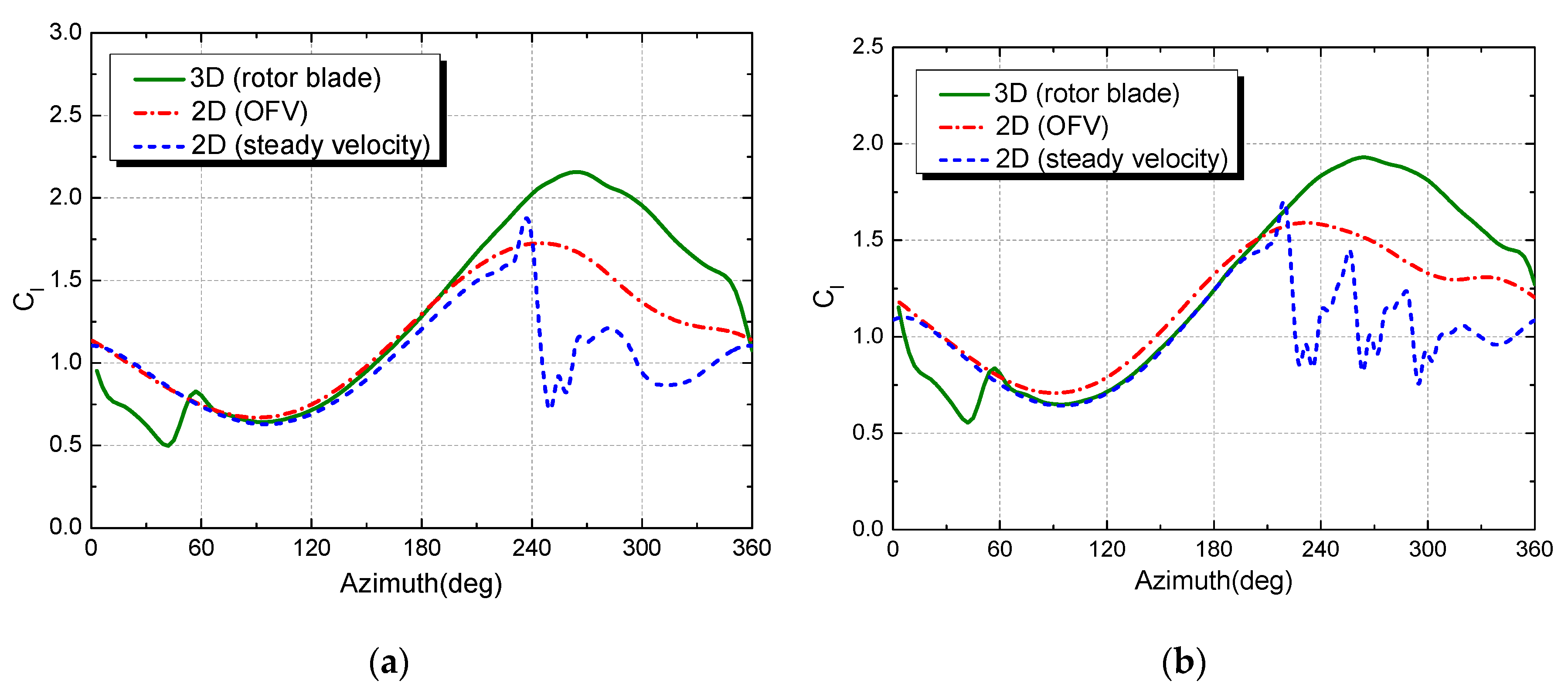
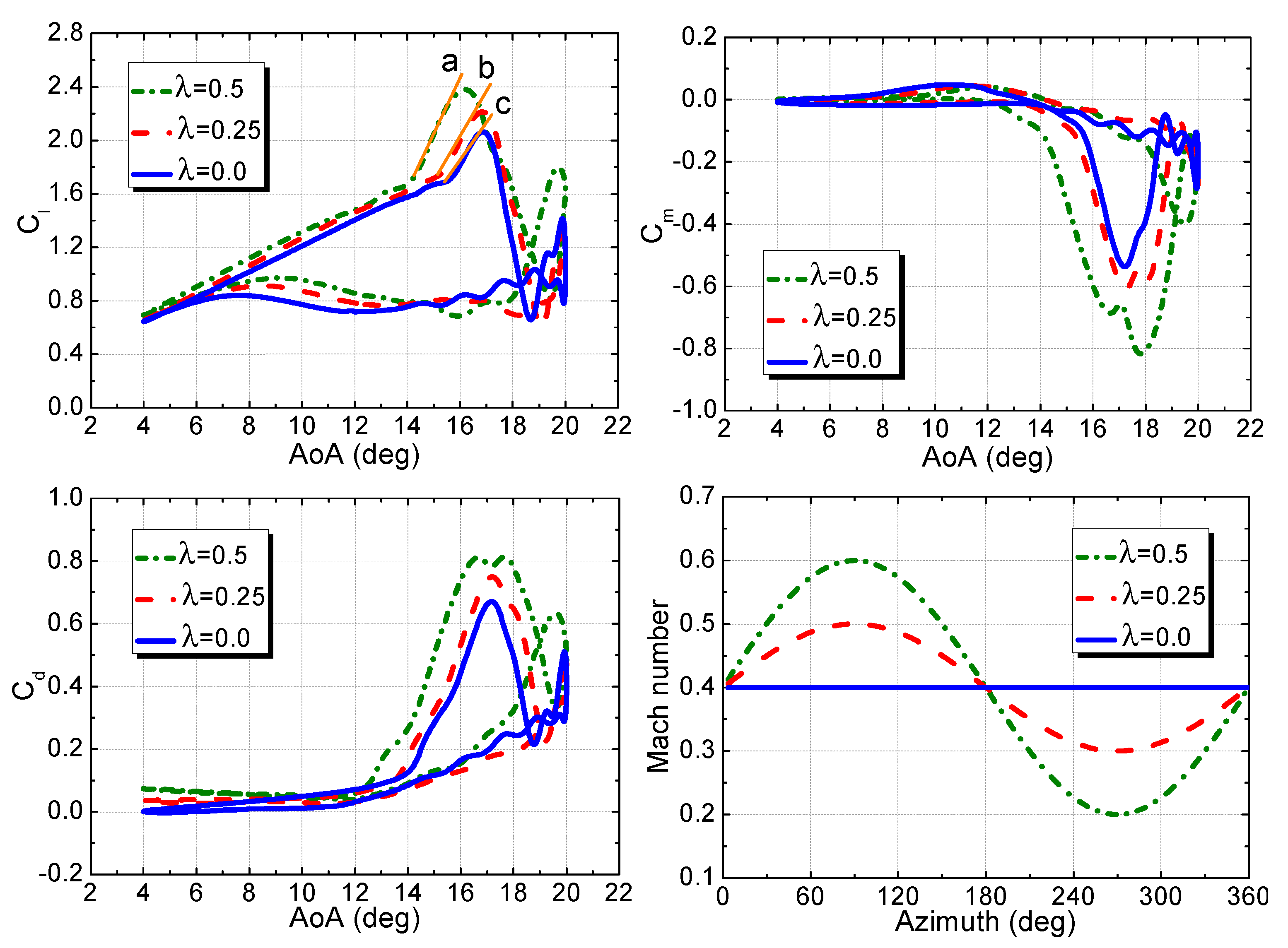
4.2. Aerodynamic Loads of Airfoil under Coupled Condition

Generally, the adverse pressure gradient near the leading edge of airfoil would be enlarged by increasing the AoA at fixed freestream velocity. On the contrary, it would be reduced by decreasing the freestream velocity at fixed AoA. Therefore, the dynamic stall characteristics of airfoil would be affected by both AoA and freestream velocity. In order to explore these characters more deeply, two cases of dynamic stall coupled with OFV are presented in this research.

4.2.1. Case 1

In this case, the dynamic stall characteristics of the OA209 airfoil are simulated at $\alpha ={12.0}^{°}+{8.0}^{°}\sin (\omega t+\pi )$ with reduced frequency of 0.075, the basic Mach number is M_B = 0.4, and $\lambda$ = 0.0, 0.25, and 0.5, respectively. The variation of Mach number with AoA is shown in Figure 9, where $\lambda$ = 0.0 represents the case of steady velocity.

The streamlines and pressure contour around the OA209 airfoil under the coupled conditions are shown in Figure 10. It can be seen that the LEV at the AoA of 12.84° during the upstroke process is not obvious under the SFV condition. However, the LEV is observed near the leading edge of airfoil for the state of $\lambda =0.5$. It is indicated that the LEV would form earlier under the condition of OFV. Due to the induction of LEV and the influence of trailing edge of airfoil, the trailing edge vortex (TEV) forms near the trailing edge of airfoil. The AoAs of LEV and TEV formation are shown in

Table 2. AoAs of leading edge vortex (LEV) and trailing edge vortex (TEV) formation.

	$\mathit{\lambda }=0.0$	$\mathit{\lambda }=0.25$	$\mathit{\lambda }=0.5$
LEV	14.47°	14.07°	12.84°
TEV	15.25°	14.87°	13.66°

. It is illustrated that the AoAs of LEV and TEV formation are both decreased with the increase of normalized oscillating velocity.

Figure 11 shows the pressure coefficient (Cp₂, normalized by ${\rho }_{\infty }{a}_{\infty }^2/2$) of the OA209 airfoil on the upper surface through a pitching cycle. It is illustrated that the Cp₂ near the leading edge of airfoil under the OFV condition is smaller than that under the SFV condition at the same AoA between the azimuth of 60° to 180°, because the increase of freestream velocity under the OFV condition would enlarge the pressure. What is more, another feature can be noticed in that the negative pressure peak is restricted at Cp₂ = −1.08 due to the effect of the LEV.

The aerodynamic loads of the OA209 airfoil are shown in Figure 12. It can be noticed that the C_l is increased by enlarging the normalized oscillating velocity during the upstroke process, and the lift curve slopes at a large AoA, for the different oscillating velocities are 0.371 (line a for $\lambda =0.5$), 0.273 (line b for $\lambda =0.25$) and 0.228 (line c for $\lambda =0.0$), respectively. As a result, the peaks of C_l are also enlarged under the OFV condition. This characteristic indicates that lift induced by LEV would be enlarged as the oscillating velocity increases. From

Table 3. Peaks of the aerodynamic loads.

Loads	$\mathit{\lambda }=0.0$		$\mathit{\lambda }=0.25$		$\mathit{\lambda }=0.5$
	Peak	Increment	Peak	Increment	Peak	Increment
Cl	2.06	0.0	2.21	7.3%	2.38	15.5%
Cd	0.67	0.0	0.75	11.9%	0.81	20.9%
Cm	−0.54	0.0	−0.61	13.0%	−0.82	51.9%

, it is illustrated that the peak of C_l with $\lambda =0.5$ is 14.5% higher than that of $\lambda =0.0$. Meanwhile, the divergence angles of the C_m and C_d are decreased when the oscillating velocity increases. Additionally, the peaks of C_m and C_d loops under the OFV condition are also larger than that of the SFV condition, and the peak values are shown in Table 3. Therefore, it is illustrated that the unsteady aerodynamic characteristics of airfoil under the OFV condition can be aggravated due to the effects of dynamic stall vortex.

4.2.2. Case 2

The dynamic stall under the coupled condition with k = 0.05 and $\alpha ={10.0}^{°}+{6.0}^{°}\sin (\omega t+\pi )$ is presented in this case. The comparisons of aerodynamic loads are shown in Figure 13. It is illustrated that the dynamic stall characteristics of the OA209 airfoil is obviously alleviated under the OFV condition (i.e., the hysteresis loop area of the dynamic stall is decreased). Meanwhile, this tendency is enhanced by increasing the oscillating velocity (i.e., the stall AoA of C_l is postponed from 14.4° ($\lambda =0.0$) to 15.6° ($\lambda =0.5$)). Moreover, the peaks of C_m and C_d under the condition of $\lambda =0.5$ are −0.002 and 0.089, which are much smaller than the peaks of C_m and C_d at $\lambda =0.0$(−0.302 and 0.356, respectively). This variation is obviously different from case 1 (i.e., the deep dynamic stall condition), since the adverse pressure gradient caused by AoA increment would be inhibited due to the effect of freestream Mach number decrement at a larger angle of attack. As a result, the LEV generation would be restricted under the light dynamic stall condition. Even more, the LEV would be eliminated under the large oscillating velocity condition. As shown in Figure 14, it can be seen that there are three LEVs shed under the SFV condition. However, there are no LEVs shed from the leading edge of the airfoil under the condition of $\lambda =0.5$. It also can be noticed that the pressure coefficient variation (normalized by ${\rho }_{\infty }{a}_{\infty }{}^2/2$) near the leading edge of airfoil under the OFV condition is milder compared with those under the SFV condition. For the case of $\lambda =0.5$, the maximum negative pressure is −0.98, which is smaller than the maximum negative pressure (−1.08) at $\lambda =0.0$.

By comparing the simulated results in these two cases, it is indicated that the dynamic stall characteristics of airfoil are associated with the pressure near the leading edge of airfoil, which would induce airflow separation and form a LEV. If the maximum pressure exceeds the critical value of leading edge separation under dynamic stall conditions, the unsteady characteristics would be enhanced with increased oscillating velocity. Otherwise, the dynamic stall characteristics would be inhibited, because the increment of adverse pressure gradient due to the increase of AoA would be restricted by decreasing freestream velocity.

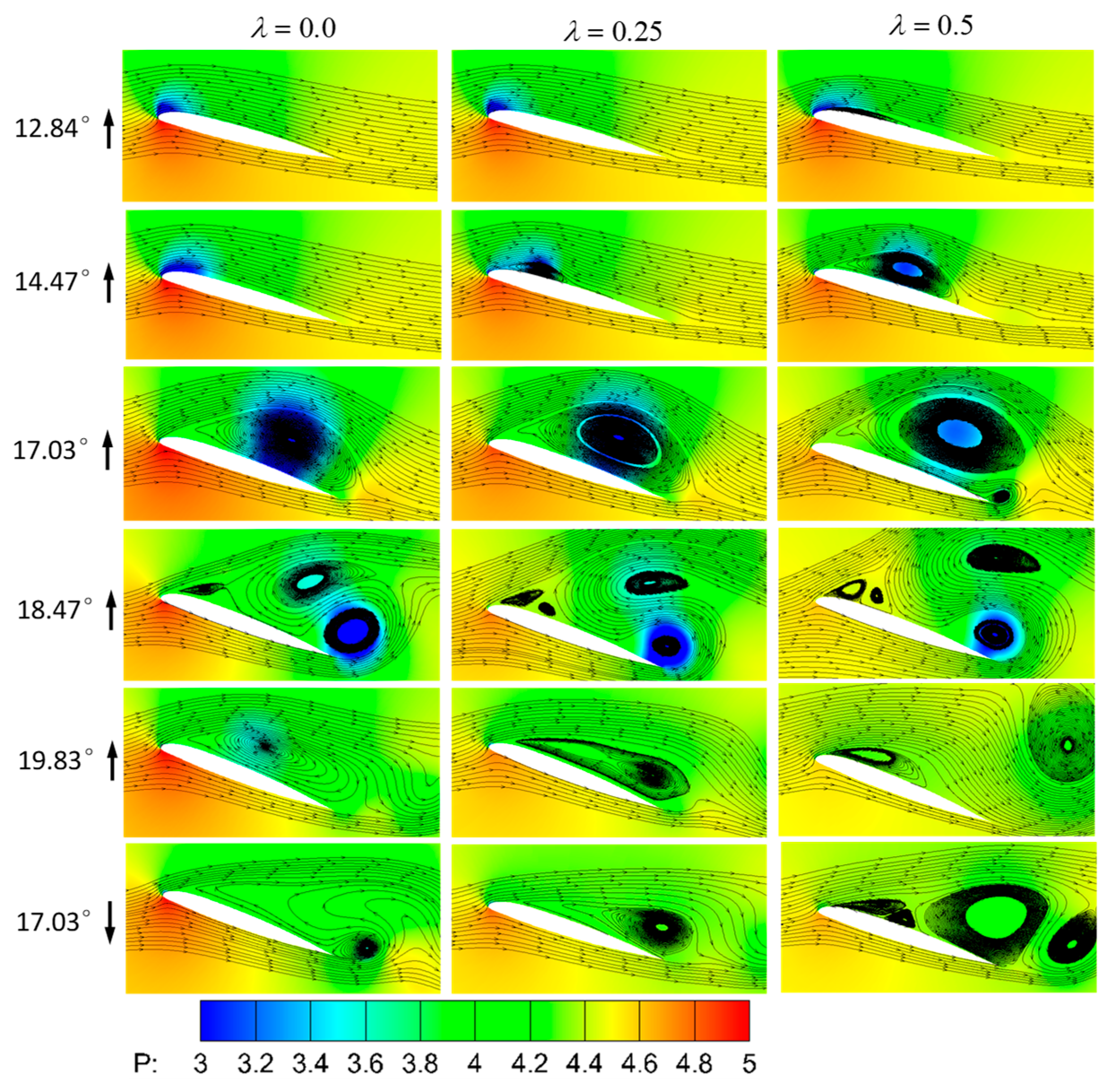
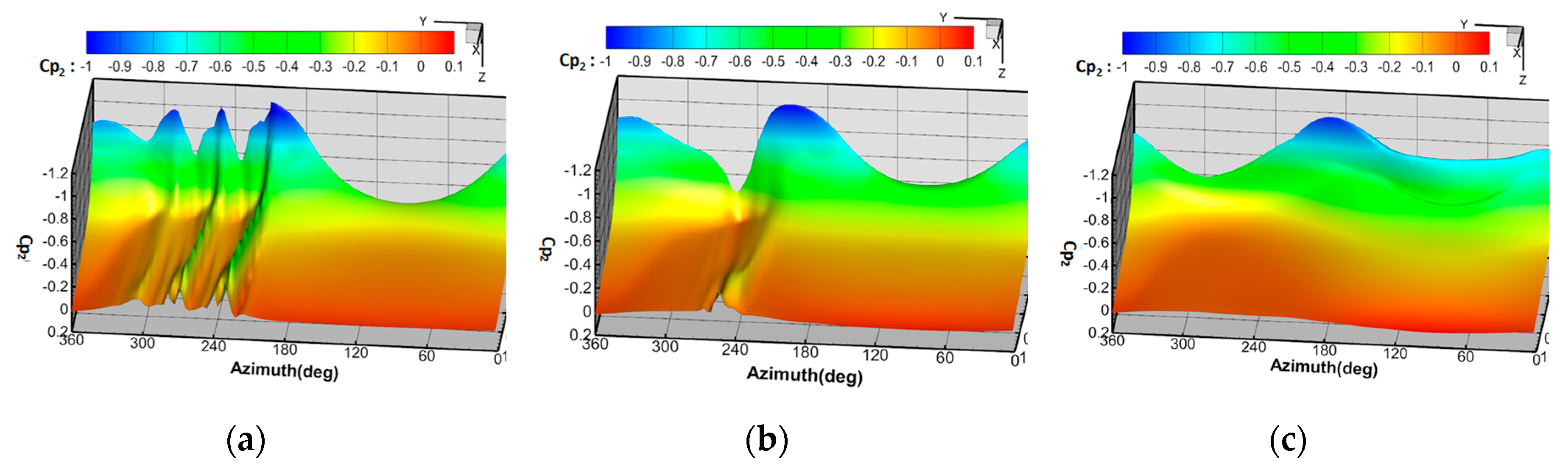
4.3. Vortex Characters of Dynamic Stall under the OFV Condition

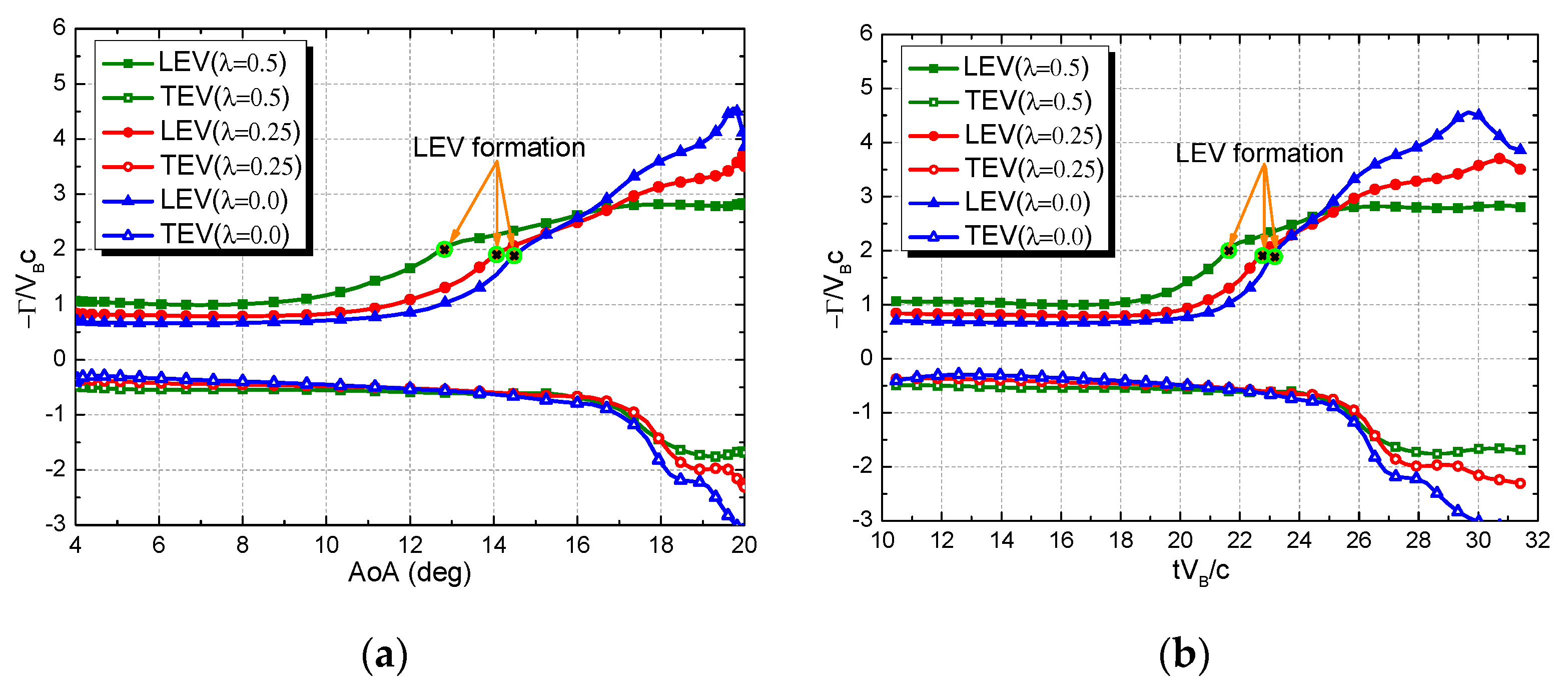
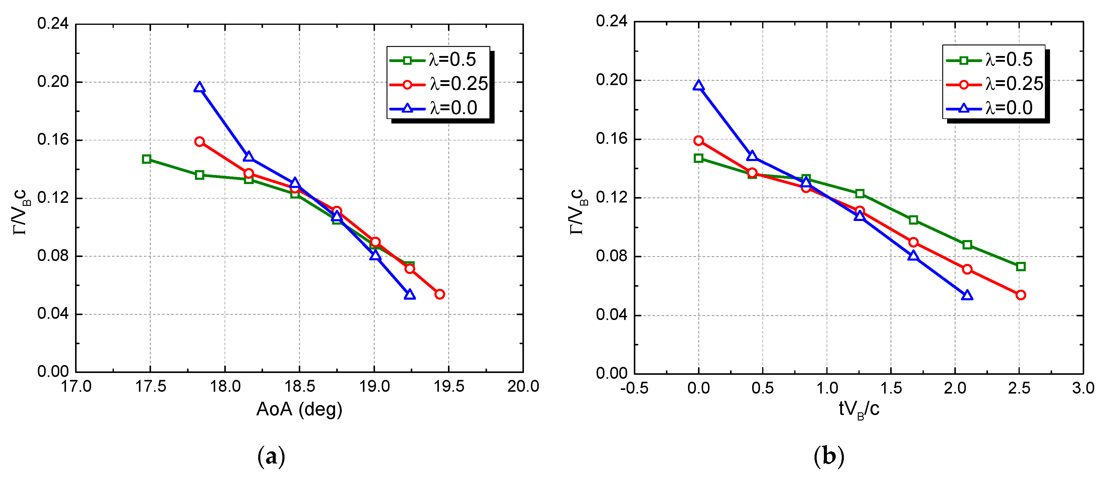
4.3.1. Circulation of Flowfield

Aimed at investigating the characteristics of a separated vortex, the circulation of flowfield is estimated from the local vorticity field via numerical integration based on Stokes’ theorem [39]:

$$\mathsf{\Gamma }={\displaystyle {\iint }_A{\omega }_z}dA$$

(8)

where A represents the integral window encompassing the vortex, ${\omega }_z$ represents the vorticity. In order to research the vorticity variation of LEV and TEV, the circulations are integrated in the simulated flowfield (${\omega }_z<0.0$ for the LEV, and ${\omega }_z>0.0$ for the TEV). Meanwhile, the vorticity in the boundary layer is neglected in the integration. Since the second vortex induced by the LEV usually has the same rotation as the TEV, the TEV integral window is started behind 0.6c position of airfoil to eliminate the interference of the second vortex, just as shown in Figure 15.

The variations of circulation at different oscillating velocities on upstroke process are shown in Figure 16, and the simulated state is the same as case 1 (i.e., k = 0.075, $\alpha ={12.0}^{°}+{8.0}^{°}\sin (\omega t+\pi )$). It can be seen from Figure 16a that the circulation of LEV at $\lambda =0.0$ is less than that under the OFV condition when the AoA is smaller than 15.5°, because the flowfield under the SFV condition is more stable. Meanwhile, it is indicated that the AoAs of LEV formation are decreased by increasing the oscillating velocity, since the variation of freestream velocity could increase the instability of the boundary layer of airfoil, which induces the airflow separation easily. Meanwhile, it can be seen from Figure 16b that the LEV generates earlier under OFV conditions compared with SFV conditions. However, the accumulating rate of LEV circulation at $\lambda =0.25$ and $\lambda =0.5$ is smaller than the circulation at $\lambda =0.0$, because the freestream velocity is decreased when the AoA increases under the OFV condition, which could reduce the energy supplement from the airflow into the LEV. As a result, the circulation would be decreased with the increase of oscillating freestream velocity. In addition, it also can be seen that the circulation of TEV has the same variational characters due to the circulation conservation of flowfield. Therefore, it is indicated that the circulation variations under the OFV condition are milder compared with the SFV condition.

In order to analyze the dynamic stall vortex characteristics deeply, Figure 17 shows the circulation variations of case 2 (i.e., k = 0.05, $\alpha ={10.0}^{°}+{6.0}^{°}\sin (\omega t+\pi )$), at different oscillating velocities. It is illustrated in this figure that the circulation of LEV at $\lambda =0.0$ obviously increases when the AoA is larger than 12.0°. However, the circulation of LEV at $\lambda =0.5$ almost keeps stable at different AoAs (Figure 17a) or times (Figure 17b). It is indicated that the LEV is basically eliminated in the state of $\lambda =0.5$. In addition, it also can be seen that the circulation of TEV is also stable for this case due to the circulation conservation of the flowfield. As a result, the dynamic stall characteristics of airfoil would be alleviated under the OFV condition with light dynamic stall, and this variational characteristic is similar to the aerodynamic loads.

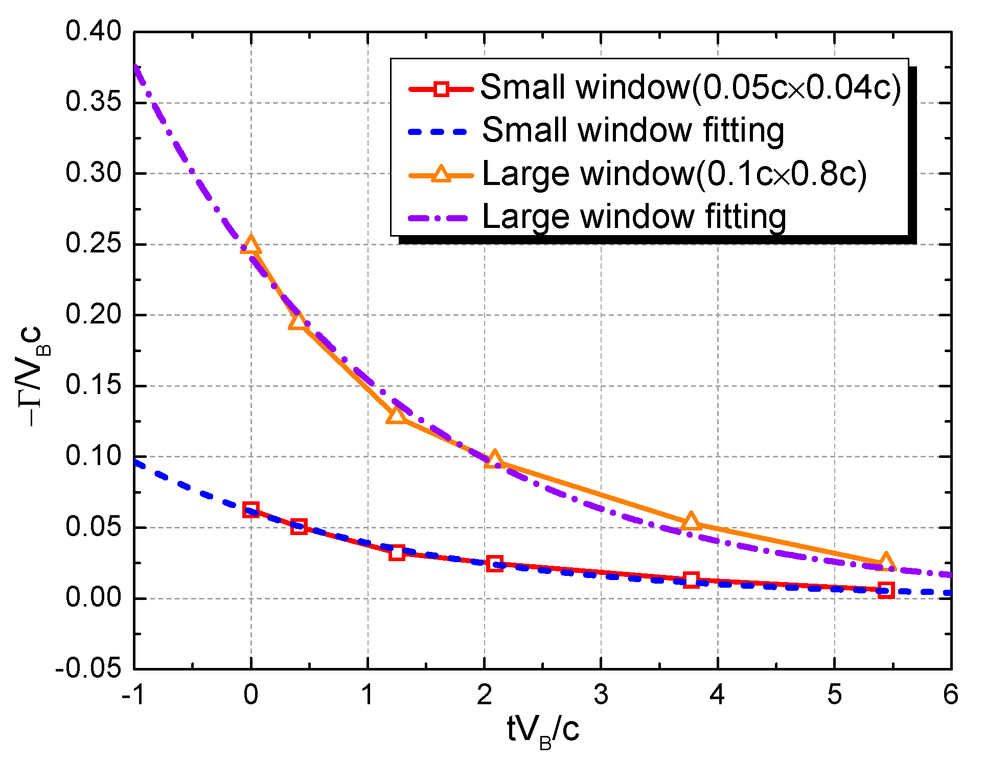
4.3.2. Dissipation Process of Separated Vortex

Since the separated vortex has significant influence on airfoil unsteady aerodynamic force characteristics, the vortex circulation near the upper surface should be researched deeply. As a result, in order to explore the dissipation process of the separated vortex, the integration with fixed windows is accomplished in this research, and the region of integral windows is 0.1 c × 0.08 c for LEV, and 0.08 c × 0.08 c for TEV at different AoAs, just as shown in Figure 18. The dissipation of vortex circulation can be expressed as

$$\mathsf{\Gamma }={\mathsf{\Gamma }}_0{e}^{-\kappa t}$$

(9)

where ${\mathsf{\Gamma }}_0$ denotes original vortex circulation, $\kappa$ denotes dissipation coefficient of LEV.

In order to analyze the influence of the integral windows on the dissipation process of the vortex, the circulation of LEV is estimated in different integral windows (i.e., 0.1 c × 0.08 c (large window) and 0.05 c × 0.04 c (small window)), then the variations of the LEV circulations of case 1 with $\lambda =0.5$ are shown in Figure 19. By fitting the samples of LEV circulation, the dissipation coefficients ($\kappa$) of LEV for different integral windows are 0.447 for 0.1 c × 0.08 c and 0.451 for 0.05 c × 0.04 c, respectively. It is indicated that the dissipation rate of LEV with different integral windows is similar.

The dissipation process of LEV circulation in Figure 20a illustrates that the circulation of LEV under the OFV condition is smaller than that under the SFV condition at the same AoA. Therefore, it is indicated that the LEV forms and sheds at smaller AoAs under the OFV condition, and this tendency accelerates with the increase in oscillating velocity. In order to explore the dissipation rate of LEV, the variations of LEV circulation with time are shown in Figure 20b. It is illustrated that the dissipation rates of different LEVs are almost the same. As a result, a new dissipation coefficient for different freestream velocities is calculated by fitting the three group vortexes (i.e., $\kappa =0.426$(${\mathsf{\Gamma }}_0=0.228$)). It is indicated that the oscillating velocity has no obvious influence on the dissipation rate of LEV. The variations of TEV circulation are shown in Figure 21. It is illustrated that the dissipation rate of TEV under the condition of OFV is slower than that under the SFV condition. This tendency could be attributed to the reason that the freestream velocity under the OFV condition is smaller than that under the SFV condition when the TEV is forming. Therefore, more energy would be supplied to the TEV from the lower surface of the airfoil since the TEV has a longer attachment time. Consequently, the dissipation rate of TEV decreased under the OFV condition.

5. Conclusions

An unsteady numerical method incorporated with the moving-embedded grid method is developed to simulate dynamic stall characteristics of a rotor airfoil under OFV conditions, and two conclusions can be summarized as:

(1).

By comparing the simulated result, it is indicated that the dynamic stall characteristics of the OA209 airfoil would be enhanced with increased oscillating velocity when the maximum negative pressure exceeds the critical value (−1.08). On the contrary, it would be inhibited when the maximum negative pressure is less than this critical value.

(2).

By comparing the dissipation processes of vortex circulation at a fixed integral window, it indicates that the dissipation of LEV presents as exponent characteristics under different oscillating velocities. Meanwhile, the dissipation rate of LEV is not sensitive to different oscillating velocities. However, the dissipation rate of TEV would be reduced by increasing the oscillating velocity.

References

1. Conlisk, A.T. Modern Helicopter Aerodynamics. Annu. Rev. Fluid Mech. 1997, 29, 515–567. [Google Scholar] [CrossRef]
2. Leishman, J.G. Principles of Helicopter Aerodynamics; Cambridge University Press: New York, NY, USA, 2006. [Google Scholar]
3. McCroskey, W.J.; Carr, L.W.; McAlister, K.W. Dynamic Stall Experiments on Oscillating Airfoil. AIAA J. 1976, 14, 57–63. [Google Scholar] [CrossRef]
4. Geissler, W.; Haselmeyer, H. Investigation of Dynamic stall Onset. Aerosp. Sci. Technol. 2006, 10, 590–600. [Google Scholar] [CrossRef]
5. Baik, Y.S.; Rausch, J.M.; Bernal, L.P. Experimental Investigation of Pitching and Plunging Airfoils at Reynolds Number Between 1×10⁴ and 6×10⁴. In Proceedings of the 39th AIAA Fluid Dynamics Conference, San Antonio, TX, USA, 22–25 June 2009. [Google Scholar]
6. Naughton, J.; Strike, J.; Hind, M.; Magstadt, A.; Babbitt, A. Measurements of Dynamic Stall on the DU Wind Turbine Airfoil Series. In Proceedings of the 69th American Helicopter Society Annual Forum, Phoenix, AZ, USA, 21–23 May 2013. [Google Scholar]
7. Beddoes, T.S. Representation of Airfoil Behaviour. Vertica 1983, 7, 183–197. [Google Scholar]
8. Leishman, J.G. Validation of Approximate Indicial Aerodynamic Functions for Two-Dimensional Subsonic Flow. J. Aircr. 1988, 25, 914–922. [Google Scholar] [CrossRef]
9. Ramesh, K.; Gopalarathnam, A.; Granlund, K.; Ol, M.V.; Edwards, J.R. Discrete-vortex Method with Novel Shedding Criterion for Unsteady Aerofoil Flows with Intermittent Leading-edge Vortex Shedding. J. Fluid Mech. 2014, 751, 500–538. [Google Scholar] [CrossRef]
10. Ramesh, K.; Murua, J.; Gopalarathnam, A. Limit-cycle Oscillations in Unsteady Flows Dominated by Intermittent Leading-edge Vortex Shedding. J. Fluids Struct. 2015, 55, 84–105. [Google Scholar] [CrossRef] [Green Version]
11. Narsipur, S.; Gopalarathnam, A.; Edwards, J.A. A Time-Lag Approach for Prediction of Trailing Edge Separation in Unsteady Flow. In Proceedings of the 32nd AIAA Applied Aerodynamics Conference, Atlanta, GA, USA, 16–20 June 2014. [Google Scholar]
12. Narsipur, S.; Gopalarathnam, A.; Edwards, J.A. Low-Order Modeling of Airfoils with Massively Separated Flow and LeadingEdge Vortex Shedding. In Proceedings of the 2018 AIAA Aerospace Sciences Meeting, Kissimmee, FL, USA, 8–12 January 2018. [Google Scholar]
13. Costes, M.; Richez, F.; Le Pape, A.; Gavériaux, R. Numerical Investigation of Three-dimensional Effects During Dynamic stall. Aerosp. Sci. Technol. 2015, 47, 216–237. [Google Scholar] [CrossRef]
14. AlMutairi, J.; ElJack, E.; AlQadi, I. Dynamics of Laminar Separation Bubble over NACA-0012 Airfoil Near Stall Conditions. Aerosp. Sci. Technol. 2017, 68, 193–203. [Google Scholar] [CrossRef]
15. Amiri, H.A.; Shafaghat, R.; Alamian, R.; Taheri, S.M. Study of horizontal axis tidal turbine performance and investigation on the optimum fixed pitch angle using CFD: A case study of Iran. Int. J. Numer. Methods Heat Fluid Flow 2020, 30, 206–227. [Google Scholar] [CrossRef]
16. Favier, D.; Maresca, C.; Rebont, J. Dynamic Stall Due to Fluctuations of Velocity and Incidence. AIAA J. 1982, 20, 865–871. [Google Scholar] [CrossRef]
17. Gursul, I.; Ho, C.M. High Aerodynamic Loads on An Airfoil Submerged in An Unsteady Stream. AIAA J. 1992, 30, 1117–1119. [Google Scholar] [CrossRef]
18. Gursul, I.; Lin, H.; Ho, C.M. Effects of Time Scales on Lift of Airfoils in An Unsteady Stream. AIAA J. 1994, 32, 797–801. [Google Scholar] [CrossRef]
19. Gharali, K.; Johnson, D.A. Dynamic Stall Simulation of a Pitching Airfoil Under Unsteady Freestream Velocity. J. Fluids Struct. 2013, 42, 228–244. [Google Scholar] [CrossRef]
20. Gompertz, K.A.; Jensen, C.D.; Gregory, J.W.; Bons, J.P. Compressible Dynamic Stall Mechanisms Due to Airfoil Pitching and Freestream Mach Oscillations. In Proceedings of the 68th American Helicopter Society Annual Forum, Fort Worth, TX, USA, 1–3 May 2012. [Google Scholar]
21. Hird, K.; Frankhouser, M.W.; Gregory, J.W.; Bons, J.P. Compressible Dynamic Stall of an SSC-A09 Airfoil Subjected to Coupled Pitch and Freestream Mach Oscillations. In Proceedings of the 70th American Helicopter Society Annual Forum, Montreal, QC, Canada, 20–22 May 2014. [Google Scholar]
22. Wong, J.G.; Mohebbian, A.; Kriegseis, J.; Rival, D.E. Rapid Flow Separation for Transient Inflow Conditions Versus Accelerating Bodies: An Investigation into Their Equivalency. J. Fluids Struct. 2013, 40, 257–268. [Google Scholar] [CrossRef]
23. Jones, A.; Hodara, J.; Smith, M.; Granlund, K.; Mulleners, K.; Ol, M. Blade Sections in Streamwise Oscillations into Reverse Flow. In Proceedings of the 71st American Helicopter Society Annual Forum, Virginia Beach, VA, USA, 5–7 May 2015. [Google Scholar]
24. Mulleners, K.; Ol, M.; Jones, A. Experimental Analysis of the Flow Development on An Airfoil Harmonically Surging into Reverse Flow. In Proceedings of the AIAA SciTech, San Diego, CA, USA, 4–8 January 2016. [Google Scholar]
25. Granlund, K.; Ol, M.; Monnier, B.; Williams, D. Airfoil Longitudinal Gust Response in Separated vs. Attached Flows. In Proceedings of the 42nd AIAA Fluid Dynamics Conference and Exhibit, New Orleans, LA, USA, 25–28 June 2012. [Google Scholar]
26. Ahmad, J.; Duque, E.P.N. Helicopter Rotor Blade Computation in Unsteady Flows Using Moving Overset Grids. J. Aircr. 1996, 33, 54–60. [Google Scholar] [CrossRef]
27. Pomin, H.; Wagner, S. Navier-Stokes Analysis of Helicopter Rotor Aerodynamics in Hover and Forward Flight. J. Aircr. 2001, 39, 813–821. [Google Scholar] [CrossRef]
28. Thompson, J.F. Grid Generation Techniques in Computational Fluid Dynamics. AIAA J. 1984, 22, 1505–1523. [Google Scholar] [CrossRef]
29. Zhao, Q.J.; Xu, G.H.; Zhao, J.G. New Hybrid Method for Predicting the Flowfields of Helicopter Rotors. J. Aircr. 2006, 43, 372–380. [Google Scholar] [CrossRef]
30. Wang, Q.; Zhao, Q.J. Unsteady Aerodynamic Characteristics Investigation of Rotor Airfoil Under Variational Freestream Velocity. Aerosp. Sci. Technol. 2016, 58, 82–91. [Google Scholar] [CrossRef]
31. Zhao, Q.J.; Zhao, G.Q.; Wang, B.; Wang, Q.; Shi, Y.J.; Xu, G.H. Robust Navier-Stokes method for predicting unsteady flowfield and aerodynamic characteristics of helicopter rotor. Chin. J. Aeronaut. 2018, 31, 214–224. [Google Scholar] [CrossRef]
32. Yoon, S.; Jameson, A. Lower-Upper Symmetric-Gauss-Seidel Method for The Euler and Navier-Stokes Equations. AIAA J. 1988, 26, 1025–1026. [Google Scholar] [CrossRef] [Green Version]
33. Stoll, P.; Gerlinger, P.; Bruggemann, D. Domain Decomposition for An Implicit LU-SGS Scheme Using Overlapping Grids. In Proceedings of the 13th Computational Fluid Dynamics Conference, Snowmass Village, CO, USA, 29 June–2 July 1997; pp. 97–1896. [Google Scholar]
34. Wadcock, A.J. Flying-Hot-Wire Study of Two-Dimensional Turbulent Separation on an NACA4412 Airfoil at Maximum Lift. Ph.D. Thesis, California Institute of Technology, Pasadena, CA, USA, 1978. [Google Scholar]
35. McAlister, K.W.; Pucci, S.L.; McCroskey, W.J.; Carr, L.W. An. Experimental Study of Dynamic Stall on Advanced Airfoil Sections Volume 2: Pressure and Force Data; NASA TM-84245; NASA: Moffett Field, CA, USA, 1982.
36. Van der Wall, B.G.; Leishman, J.G. On the Influence of Time-Varying Flow Velocity on Unsteady Aerodynamics. J. Am. Helicopter Soc. 1994, 39, 25–36. [Google Scholar] [CrossRef]
37. Heffernan, R.M.; Gaubert, M. Structural and Aerodynamic Loads and Performance Measurements of an SA349/2 Helicopter with an Advanced Geometry Rotor; NASA TM-88370; NASA: Moffett Field, CA, USA, 1 November 1986.
38. Gardner, A.D.; Richter, K. Influence of Rotation on Dynamic Stall. In Proceedings of the 68th American Helicopter Society International Annual Forums, Fort Worth, TX, USA, 1–3 May 2012. [Google Scholar]
39. Prangemeire, T.; Rival, D.; Tropea, C. The Manipulation of Trailing-Edge Vortices for an Airfoil in Plunging Motion. J. Fluids Struct. 2010, 26, 193–204. [Google Scholar] [CrossRef]
Figure 1. Mach number distribution of rotor disk and angle of attack (AoA) variation with rotor azimuth. (a) Mach number distribution. (b) AoA and freestream velocity variations.
Applsci 10 01822 g001
Figure 2. Schematic of moving-embedded grids.
Applsci 10 01822 g002
Figure 3. Comparisons of pressure coefficient (Cp) and velocity profiles of NACA4412 airfoil with test data. (a) Cp distribution. (b) Velocity profiles.
Applsci 10 01822 g003
Figure 4. Comparison of simulated Cl with test data.
Applsci 10 01822 g004
Figure 5. Comparison of simulated results with Isaacs’s theory under the oscillating freestream velocity (OFV) condition.
Applsci 10 01822 g005
Figure 6. Comparison of normal force between the test data and numerical data. (a) r/R = 0.75. (b) r/R = 0.97.
Applsci 10 01822 g006
Figure 7. Comparison of Cp between the test data and numerical data. (a) ψ = 90°. (b) ψ = 180°. (c) ψ = 270°. (d) ψ = 360°.
Applsci 10 01822 g007
Figure 8. Comparisons of dynamic stall characteristics of airfoil between the 2D and 3D conditions. (a) Section of 0.6 R. (b) Section of 0.7 R.
Applsci 10 01822 g008
Figure 9. Comparison of Mach number variation with AoA.
Applsci 10 01822 g009
Figure 10. Comparisons of pressure contour and streamlines at different oscillating velocities (k = 0.075, α = 12.0 ° + 8.0 ° sin ( ω t + π ) ).
Applsci 10 01822 g010
Figure 11. Comparisons of pressure coefficient at different oscillating velocities (k = 0.075, α = 12.0 ° + 8.0 ° sin ( ω t + π ) ). (a) λ = 0.0 . (b) λ = 0.25 . (c) λ = 0.5 .
Applsci 10 01822 g011
Figure 12. Comparisons of aerodynamic loads at different oscillating velocities (k = 0.075, α = 12.0 ° + 8.0 ° sin ( ω t + π ) ).
Applsci 10 01822 g012
Figure 13. Comparisons of aerodynamic loads at different oscillating velocities (k = 0.05, α = 10.0 ° + 6.0 ° sin ( ω t + π ) ).
Applsci 10 01822 g013
Figure 14. Comparisons of pressure coefficient with different oscillating velocities (k = 0.05, α = 10.0 ° + 6.0 ° sin ( ω t + π ) ). (a) λ = 0.0 . (b) λ = 0.25 . (c) λ = 0.5 .
Applsci 10 01822 g014
Figure 15. Integral windows of vortex circulation.
Applsci 10 01822 g015
Figure 16. Comparisons of vortex circulation between different oscillating velocities (case 1). (a) Variation with AoA. (b) Variation with time.
Applsci 10 01822 g016
Figure 17. Comparisons of vortex circulation between different oscillating velocities (case 2). (a) Variation with AoA. (b) Variation with time.
Applsci 10 01822 g017
Figure 18. Integral windows of vortex circulation with fixed windows.
Applsci 10 01822 g018
Figure 19. Comparisons of LEV dissipation between different integral windows ( λ = 0.5 ).
Applsci 10 01822 g019
Figure 20. Comparisons of LEV dissipation between different oscillating velocities. (a) Variation with AoA. (b) Variation with time.
Applsci 10 01822 g020
Figure 21. Comparisons of TEV dissipation between different oscillating velocities. (a) Variation with AoA. (b) Variation with time.
Applsci 10 01822 g021