Article

Compressed-Sensing Magnetic Resonance Image Reconstruction Using an Iterative Convolutional Neural Network Approach

1
Central Research Laboratory, Hamamatsu Photonics K.K., Hamamatsu, Shizuoka 434-8601, Japan
2
Faculty of Radiological Technology, School of Medical Sciences, Fujita Health University, Toyoake, Aichi 470-1192, Japan
3
Department of Biofunctional Imaging, Preeminent Medical Photonics Education & Research Center, Hamamatsu University School of Medicine, Hamamatsu 431-3192, Japan
*
Author to whom correspondence should be addressed.
Appl. Sci. 2020, 10(6), 1902; https://doi.org/10.3390/app10061902
Submission received: 29 January 2020 / Revised: 5 March 2020 / Accepted: 9 March 2020 / Published: 11 March 2020
(This article belongs to the Special Issue Medical Signal and Image Processing)

Abstract

:
Convolutional neural networks (CNNs) demonstrate excellent performance when employed to reconstruct the images obtained by compressed-sensing magnetic resonance imaging (CS-MRI). Our study aimed to enhance image quality by developing a novel iterative reconstruction approach that utilizes image-based CNNs and k-space correction to preserve original k-space data. In the proposed method, CNNs represent a priori information concerning image spaces. First, the CNNs are trained to map zero-filling images onto corresponding full-sampled images. Then, they recover the zero-filled part of the k-space data. Subsequently, k-space corrections, which involve the replacement of unfilled regions by original k-space data, are implemented to preserve the original k-space data. The above-mentioned processes are used iteratively. The performance of the proposed method was validated using a T2-weighted brain-image dataset, and experiments were conducted with several sampling masks. Finally, the proposed method was compared with other noniterative approaches to demonstrate its effectiveness. The aliasing artifacts in the reconstructed images obtained using the proposed approach were reduced compared to those using other state-of-the-art techniques. In addition, the quantitative results obtained in the form of the peak signal-to-noise ratio and structural similarity index demonstrated the effectiveness of the proposed method. The proposed CS-MRI method enhanced MR image quality with high-throughput examinations.

1. Introduction

Magnetic resonance imaging (MRI) is a noninvasive imaging modality for acquiring biological information at high spatial resolution. Compared to X-ray computed tomography, MRI scan times are longer owing to the use of a data-acquisition scheme that is sequentially sampled over the Fourier domain—also referred to as the k-space. This shortcoming has resulted in the proposal of several hardware-based and software-based techniques, such as asymmetric Fourier imaging [1], parallel imaging [2,3,4], and echo-planar imaging [5,6], to reduce the time required to obtain an MRI scan. However, in clinical diagnosis procedures, scanning speed must be improved without image degradation to reduce the motion artifacts caused by patients and the burden placed upon them. A possible strategy for reducing MRI scan time is to reduce the number of data acquisitions in the k-space instead of using full sampling. However, undersampled data are subject to aliasing artifacts in reconstructed images. Compressed sensing [7] can be employed for MRI reconstruction [8,9,10,11,12] using techniques that utilize sparsity in specific transform domains, such as the wavelet [8,10] and curvelet [11] transforms and dictionary learning [12], all of which have been incorporated in recently developed MRI scanners.
Even though the development of improved image-processing methods is competitive, the use of convolutional neural networks (CNNs) to enhance the quality of medical images has increasingly attracted researchers’ attention [13,14,15,16,17]. With respect to compressed-sensing MRI (CS-MRI) reconstruction, several extant studies have reported the possibility of obtaining high-quality images from undersampled data using CNNs [18,19,20,21,22,23,24] by training them to map undersampled images onto corresponding full-sampled images [18,19]. Alternatively, in a few studies, a hybrid approach that operates on both the k-space and image space has been introduced to enhance image quality [22,23]. For example, Shanshan et al. reported on the first trial of a CNN-based CS-MRI approach that can restore the brain structures from zero-filling MR images [18]. Quan et al. proposed a generative adversarial network (GAN)-based CS-MRI algorithm; however, it is difficult to train GANs stably [21]. In addition, Eo et al. proposed KIKI-net, in which CNNs operate on both the k-space and image space [22]. This approach separately minimizes the loss functions in both spaces and improves image quality by restoring tissue structures and eliminating aliasing artifacts. Hyun et al. proposed a hybrid approach that employs CNNs and k-space correction, wherein the unfilled parts of k-space data are replaced by original k-space data [23]. This approach outperforms image-based CNNs; however, aliasing artifacts still remain due to the hybrid approach. Therefore, a more effective suppression of the aliasing artifacts is greatly needed.
Our work, which was inspired by the above-mentioned research studies, involves the development of a novel iterative CNN-based method for CS-MRI reconstruction, which is presented in this paper. The method combines the operation of image-based CNNs with k-space corrections, and it demonstrates superior performance compared to standalone image-based CNN and noniterative k-space correction methods because the aliasing artifacts can be suppressed by the iterative processing of the proposed CS-MRI reconstruction. In this study, experiments were performed to analyze the quality of T2-weighted brain images that was realized using the proposed method, and image quality is expressed in terms of the peak signal-to-noise ratio (PSNR) and structural similarity index (SSIM).

2. Materials and Methods

2.1. Proposed Method

Figure 1 presents a sequential schematic of the proposed method, which iteratively processes image-based CNNs and k-space corrections, with the CNNs representing a priori image space information. The method aims to preserve information pertaining to tissue structures and to suppress aliasing artifacts to a larger degree compared to standalone image-based CNN and noniterative k-space correction methods. As indicated in Figure 1, first, undersampled k-space data, y0, are extracted from the corresponding fully sampled data using a binary sampling mask, R, and zero-filling images, x0, are obtained using the inverse Fourier transformation, 1 . Subsequently, the CNNs are trained to map these zero-filling images onto the corresponding fully sampled images, and k-space corrections are performed to replace the unsampled data by the original k-space data [23]. Finally, 1 is used to obtain the corrected images from the corrected k-space data. The above-mentioned processes are performed iteratively. Note that in all iterations except the first, CNNs are trained to map the ith output onto the corresponding fully sampled image. The calculations performed by the proposed method can be expressed by the following:
{ z i = f θ i ( | 1 ( y 0 ) | ) i = 0 z i = f θ i ( x i ) o t h e r w i s e
x i + 1 = | 1 ( y 0 + ( z i ) R ¯ ) |
Here, xi denotes the ith output of a reconstructed image, R ¯ denotes the logical negation of binary sampling mask R, denotes element-wise multiplication, and f θ represents the CNN with network weights θ . denotes the Fourier operator.

2.2. Network Architecture

Several state-of-the-art CNN architectures were previously introduced to realize efficient image-to-image transformation. The proposed approach employs a network architecture based on the 2D U-net, a detailed description of which was previously reported [25,26]. This architecture was selected owing to its known superior performance in the medical imaging field.
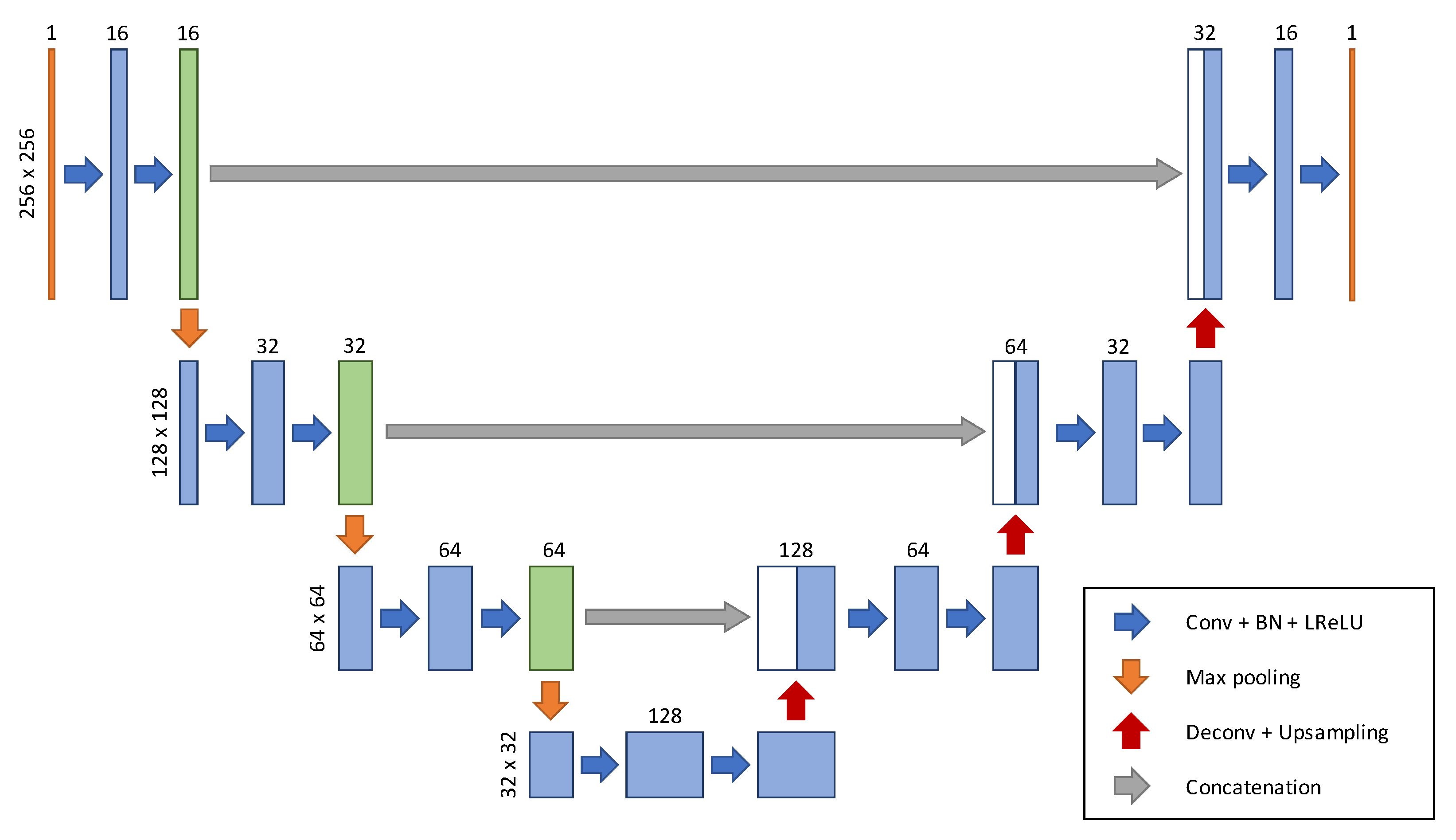
Figure 2 depicts a schematic of the 2D U-net architecture comprising independent encoding (left) and decoding (right) workflows. The encoding workflow corresponds to that of typical CNN architectures, which are constructed by repeatedly using two 3 × 3 2D convolutional layers. The processing within each such layer is followed by batch normalization (BN), the use of a leaky rectified linear unit (LReLU), and 2 × 2 max pooling for downsampling. Additionally, the number of feature channels is doubled during each downsampling step. In contrast, the decoding path comprises a 3 × 3 2D deconvolutional layer. The processing within this layer is followed by BN, an LReLU, upsampling, and skip connection with the corresponding linked-feature maps in the encoding path, and two 3 × 3 2D convolutional layers. The processing within each of these two layers is—once again—followed by BN and an LReLU. A linear function was employed to activate the output layer.
During each iteration, the above-described U-net architecture was trained using the loss function of the mean squared error, expressed by the following:
θ i = { argmin θ i x t r u e f θ i ( | 1 ( y 0 ) | ) i = 0 argmin θ i x t r u e f θ i ( x i ) o t h e r w i s e .
Here, xtrue denotes the fully sampled image corresponding to each zero-filling image. The loss function was minimized using the Adam optimizer [27] at a learning rate of 0.0001, and the number of epochs was 100. A small batch of 32 images was used for training. These hyperparameters were empirically selected. All U-net processing was performed on a computer running the Ubuntu 16.04 operating system, an NVIDIA Quadro P6000 (Sant Clara, CA, USA) graphics processing unit with 24 GB memory, TensorFlow 1.9 [28], and Keras 2.2.4 [29].

2.3. Experimental Setup

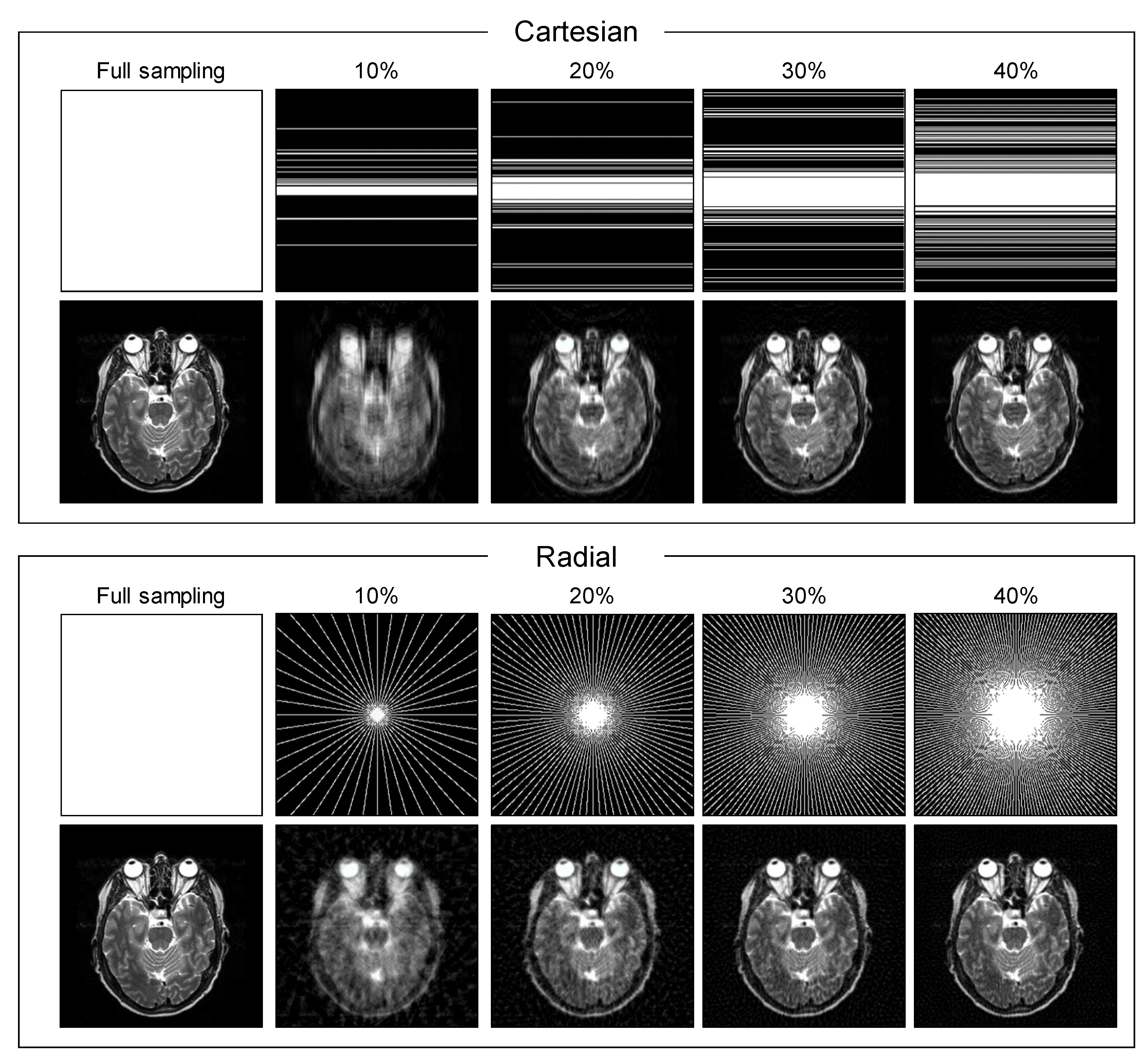
The performance of the proposed CS-MRI reconstruction approach was evaluated using a dataset comprising T2-weighted brain MR images extracted from the IXI database [30]. In this study, 7427 and 7460 images (256 × 256 resolution) of 57 subjects each were randomly selected for CNN training and testing, respectively. Experiments were performed for Cartesian and radial undersampling masks of 10%, 20%, 30%, and 40%, as indicated in Figure 3 [21].
To evaluate the performance of the proposed iterative method, the (1) standalone image-based U-net and (2) noniterative k-space correction [23] methods were adopted for comparison.
  • The standalone image-based U-net was trained by the same architecture as that of this study, expressed by the following:
    θ = argmin θ x t r u e f θ ( | 1 ( y 0 ) | ) .
  • The noniterative k-space correction method was implemented based on Hyun’s method [23], expressed by the following:
    z = f θ ( | 1 ( y 0 ) | ) ,
    x = | 1 ( y 0 + ( z ) R ¯ ) |
Here, x denotes the output of the noniterative k-space correction method that corresponds to the first output of the proposed iterative method.
To ensure a fair comparison, the architecture and hyperparameters of the CNNs of other methods were set to be identical to those considered in the proposed approach. The PSNR and SSIM values were calculated to evaluate the performance of the methods at Cartesian and radial sampling masks of different sampling rates (10%, 20%, 30%, and 40%) [31]. The statistical significance was tested by conducting a paired t-test.

3. Results

We compared the proposed method with the image-based U-net and noniterative k-space correction methods. Figure 4 presents the reconstructed results that were obtained after ten iterations of the proposed approach using Cartesian and radial sampling masks of 10%. The first to fifth columns show the ground truth, the zero-filling, image-based U-net, noniterative, and proposed methods, respectively. The proposed method can reduce aliasing artifacts compared with the other methods. The bottom row contains the error maps obtained by different methods in comparison with the fully sampled image. Even though the image-based U-net and noniterative methods can substantially reduce artifacts, the artifacts at image edges, such as those at the boundary of structures, cannot be reduced. The proposed iterative method can reduce these artifacts as well. Table 1 shows the mean and standard deviation (SD) of the PSNR and SSIM values obtained using different methods with Cartesian and radial sampling masks of 10%. Ten iterations of the proposed method resulted in statistically significant improvements (p < 0.001) in both the PSNR and SSIM compared with the other methods and the smaller iterations in the proposed method.
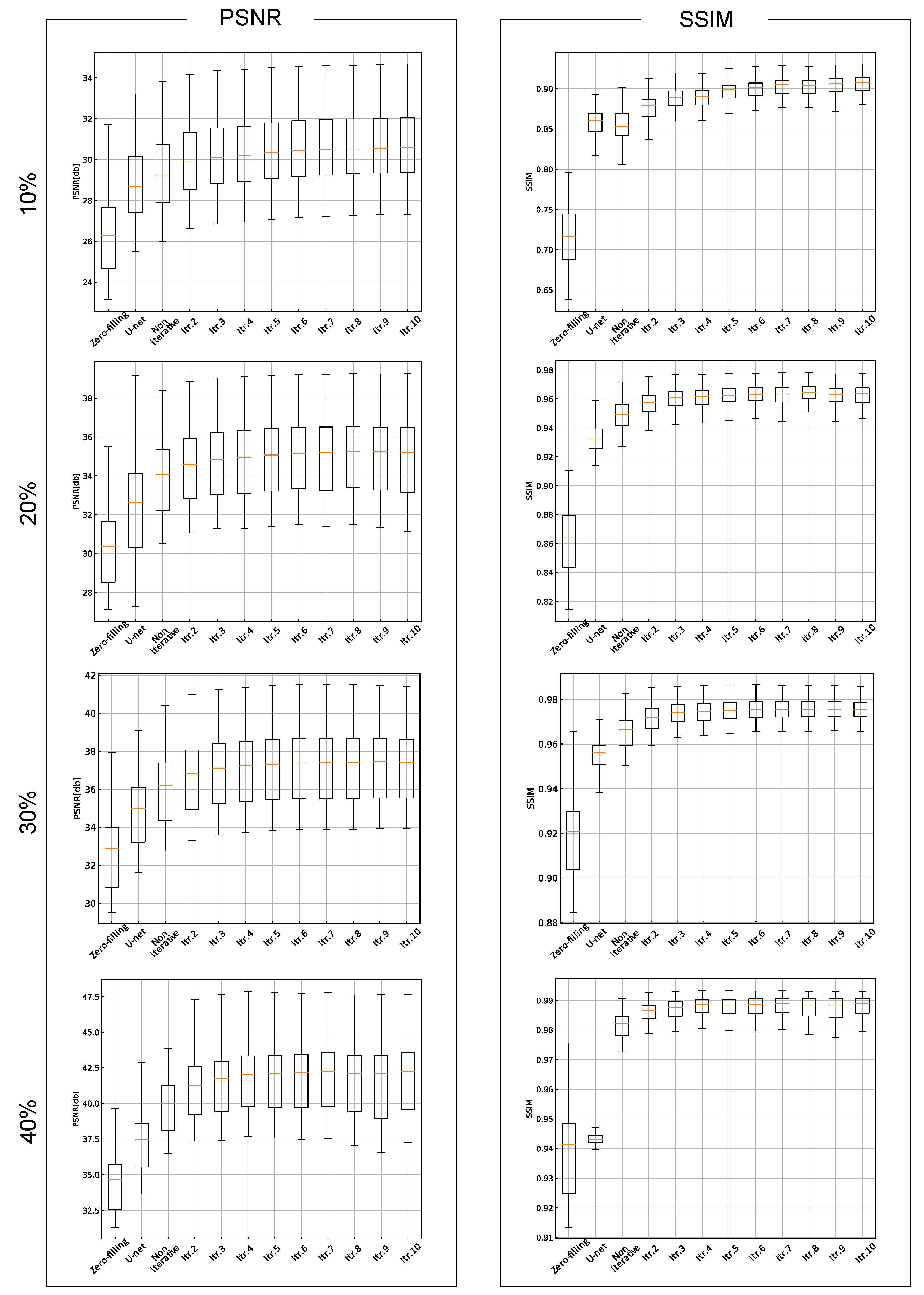
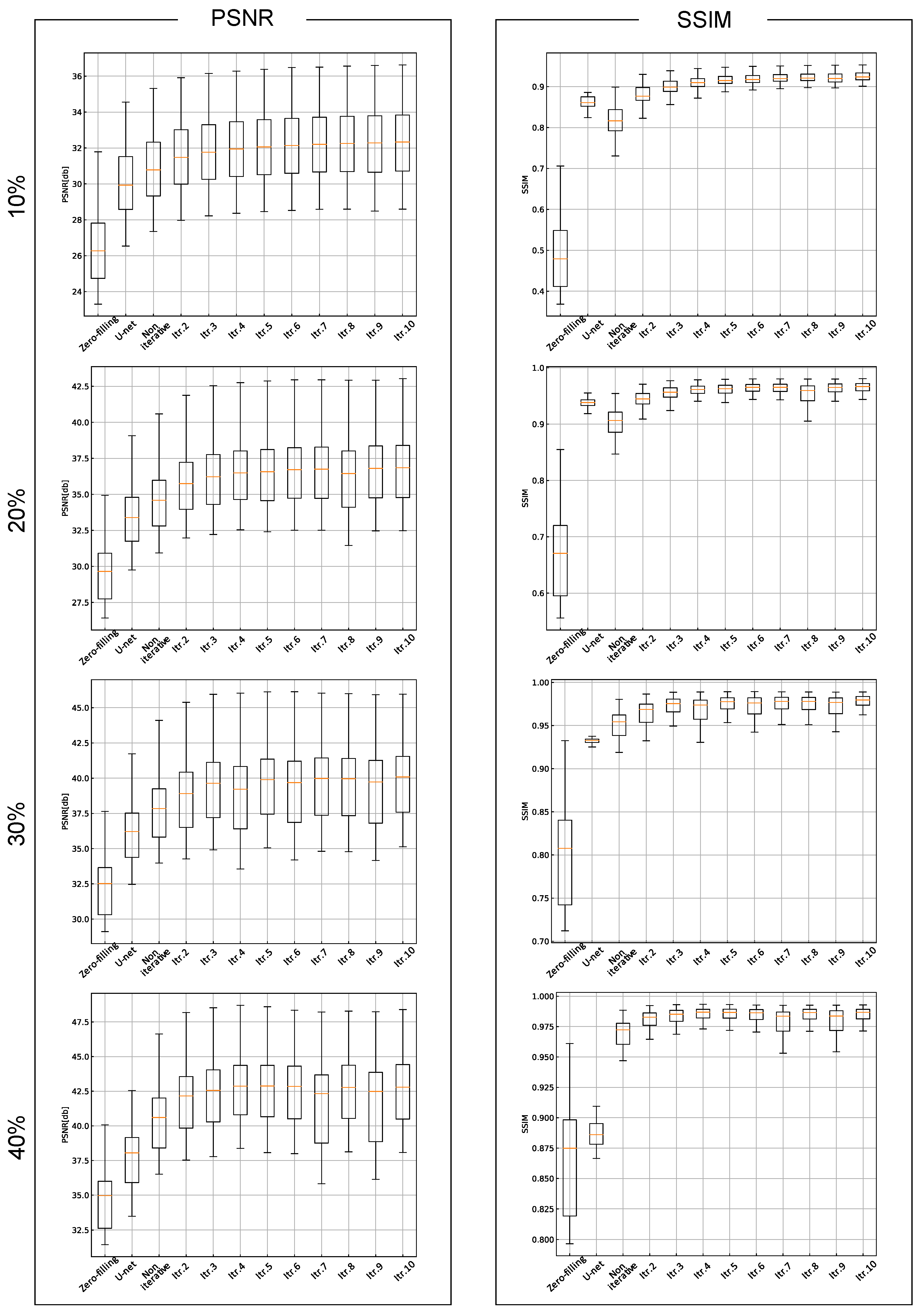
Figure 5 and Figure 6 show the box plots of the PSNR and SSIM values obtained with Cartesian and radial sampling masks of 10%, 20%, 30%, and 40%. The columns correspond to the zero-filling, image-based U-net, and noniterative methods and each iteration of the proposed method (left to right). In each plot, the yellow line within the box represents the median; the lower and upper lines of the box represent the 25th and 75th percentiles, respectively; and the lower and upper adjacent lines (whiskers) represent the minimum and maximum values, respectively. Ten iterations of the proposed method outperformed the image-based U-net and the noniterative methods for all Cartesian and radial sampling masks. In addition, the SSIMs from the noniterative method with a Cartesian sampling mask of 10% (Figure 5) and radial sampling masks of 10% and 20% (Figure 6) are lower than those from the image-based U-net and proposed methods. During training, the proposed method converges within ten iterations in terms of the PSNR and SSIM. These findings demonstrate the effectiveness of the proposed iterative method.

4. Discussion

We propose herein an iterative CNN-based method for CS-MRI reconstruction. The method combines image-based CNNs and k-space corrections, with the CNNs representing a priori image space information. The proposed method performs iterative calculations in the image and k-space domains through image restoration using the CNNs and k-space correction. In this manner, the proposed method can reduce the error in k-space correction. Compared to those obtained using other techniques, the images that are reconstructed using the proposed approach demonstrate enhanced image quality with a reduction in aliasing artifacts. The above-described results demonstrate that the proposed method outperforms the U-net trained on the image space and other noniterative methods in terms of more effective suppression of aliasing artifacts. For example, Figure 4 reveals the reconstruction errors in the ventricles of the brain for a radial sampling mask of 10%, as observed using the U-net and noniterative methods. On the contrary, the proposed method can suppress these reconstruction errors. In addition, the results obtained using the proposed method were also improved compared with those of the other methods in terms of the PSNR and SSIM for all sampling rates of the Cartesian and radial sampling masks. These results indicate that the proposed method can enhance image quality and decrease acquisition time. Additionally, the results of the quantitative evaluation reveal that, in comparison with image-based CNNs and other noniterative approaches, the proposed method increases the PSNR and SSIM for Cartesian and radial sampling masks. Particularly, at radial sampling masks of 10% and 20%, the noniterative method does not improve image quality in terms of the SSIM when compared to the U-net and proposed methods. These results support the fact that the proposed method can reduce the error in k-space correction using iterative k-space correction.
Several studies have already compared deep-learning-based methods with conventional CS-MRI algorithms. For example, Eo et al. [22] reported that a three-layered CNN based on Wang’s method [18] can achieve superior performance compared to CS-MRIs by utilizing sparsity in wavelet transforms [8] as well as dictionary learning [12]. Furthermore, the fastMRI project [32] also showed that the U-net performs substantially better than the total-variation-based CS-MRI [33]. Considering these reports, we believe that it is sufficient to compare the proposed method to the U-net and the noniterative methods.
The major limitations of the present study include the optimization of CNN hyperparameters, i.e., the number of layers, filters, epochs, and batch size. In general, these parameters are empirically determined, and the objective optimization of these parameters is necessary. In addition, the experimental data used in this study correspond to real-valued MR images, which are different from the actual k-space data obtained from an actual MRI scanner (complex-valued MR images). Hence, an imaginary channel would have to be connected to the input and output CNN layers. Alternatively, complex-valued data would have to be preprocessed. In the future, we will focus on evaluations of clinical usefulness by radiologists and testing with other MR modalities, such as T1-weighted images.

5. Conclusions

This paper presents a CS-MRI reconstruction approach that combines image-based CNNs and k-space correction, wherein the two methods are iteratively implemented, with the CNNs representing a priori image space information. The aliasing artifacts in the reconstructed images obtained using the proposed approach were reduced when compared to those obtained using other state-of-the-art techniques. In addition, the quantitative results obtained in the form of the PSNR and SSIM demonstrate the effectiveness of the proposed method. These results indicate that the proposed CS-MRI method enhances MR image quality with high-throughput examinations.

Author Contributions

Methodology, F.H., K.O. and O.T.; software, F.H.; validation, F.H.; writing—original draft preparation, F.H.; writing—review and editing, K.O., T.O., A.T. and Y.O.; supervision, A.T. and Y.O.; project administration, A.T. and Y.O. All authors have read and agreed to the published version of the manuscript.

Funding

This research received no external funding.

Acknowledgments

The authors thank the staff in the PET Research Group and the 5th Group in Central Research Laboratory, Hamamatsu Photonics K.K. for their technical suggestions.

Conflicts of Interest

The authors declare the following potential conflicts of interest with respect to the research, authorship, and/or publication of this article: F.H., K.O., and T.O. are employees of Hamamatsu Photonics K.K.

References

  1. McGibney, G.; Smith, M.R.; Nichols, S.T.; Crawley, A. Quantitative evaluation of several partial Fourier reconstruction algorithms used in MRI. Magn. Reson. Med. 1993, 30, 51–59. [Google Scholar] [CrossRef] [PubMed]
  2. Sodickson, D.K.; Manning, W.J. Simultaneous acquisition of spatial harmonics (SMASH): Fast imaging with radiofrequency coil arrays. Magn. Reson. Med. 1997, 38, 591–603. [Google Scholar] [CrossRef] [PubMed]
  3. Pruessmann, K.P.; Weiger, M.; Scheidegger, M.B.; Boesiger, P. SENSE: Sensitivity encoding for fast MRI. Magn. Reson. Med. 1999, 42, 952–962. [Google Scholar] [CrossRef]
  4. Griswold, M.A.; Jakob, P.M.; Heidemann, R.M.; Nittka, M.; Jellus, V.; Wang, J.; Kiefer, B.; Haase, A. Generalized autocalibrating partially parallel acquisitions (GRAPPA). Magn. Reson. Med. 2002, 47, 1202–1210. [Google Scholar] [CrossRef] [PubMed] [Green Version]
  5. Stehling, M.K.; Turner, R.; Mansfield, P. Echo-planar imaging: Magnetic resonance imaging in a fraction of a second. Science 1991, 254, 43–50. [Google Scholar] [CrossRef] [Green Version]
  6. Schmitt, F.; Stehling, M.K.; Turner, R. Echo-Planar Imaging: Theory, Technique and Application; Springer: Heidelberg, Germany, 1998. [Google Scholar] [CrossRef]
  7. Donoho, D.L. Compressed sensing. IEEE Trans. Inf. Theory 2006, 52, 1289–1306. [Google Scholar] [CrossRef]
  8. Lustig, M.; Donoho, D.; Pauly, J.M. Sparse MRI: The application of compressed sensing for rapid MR imaging. Magn. Reson. Med. 2007, 58, 1182–1195. [Google Scholar] [CrossRef]
  9. Gamper, U.; Boesiger, P.; Kozerke, S. Compressed sensing in dynamic MRI. Magn. Reson. Med. 2008, 59, 365–373. [Google Scholar] [CrossRef]
  10. Haldar, J.P.; Hernando, D.; Liang, Z.P. Compressed-sensing MRI with random encoding. IEEE Trans. Med. Imaging. 2010, 30, 893–903. [Google Scholar] [CrossRef] [Green Version]
  11. Ma, J. Improved iterative curvelet thresholding for compressed sensing and measurement. IEEE Trans. Instrum. Meas. 2010, 60, 126–136. [Google Scholar] [CrossRef] [Green Version]
  12. Ravishankar, S.; Bresler, Y. MR image reconstruction from highly undersampled k-space data by dictionary learning. IEEE Trans. Med. Imaging. 2010, 30, 1028–1041. [Google Scholar] [CrossRef] [PubMed]
  13. Jiang, D.; Dou, W.; Vosters, L.; Xu, X.; Sun, Y.; Tan, T. Denoising of 3D magnetic resonance images with multi-channel residual learning of convolutional neural network. Jpn. J. Radiol 2018, 36, 566–574. [Google Scholar] [CrossRef] [PubMed] [Green Version]
  14. Ran, M.; Hu, J.; Chen, Y.; Chen, H.; Sun, H.; Zhou, J.; Zhang, Y. Denoising of 3D magnetic resonance images using a residual encoder–decoder Wasserstein generative adversarial network. Med. Image Anal. 2019, 55, 165–180. [Google Scholar] [CrossRef] [Green Version]
  15. Kidoh, M.; Shinoda, K.; Kitajima, M.; Isogawa, K.; Nambu, M.; Uetani, H.; Morita, K.; Nakaura, T.; Tateishi, M.; Yamashita, Y.; et al. Deep Learning Based Noise Reduction for Brain MR Imaging: Tests on Phantoms and Healthy Volunteers. Magn. Reson. Med. Sci. 2019. [Google Scholar] [CrossRef] [Green Version]
  16. Hashimoto, F.; Ohba, H.; Ote, K.; Teramoto, A.; Tsukada, H. Dynamic PET Image Denoising Using Deep Convolutional Neural Networks Without Prior Training Datasets. IEEE Access 2019, 7, 96594–96603. [Google Scholar] [CrossRef]
  17. Du, X.; He, Y. Gradient-Guided Convolutional Neural Network for MRI Image Super-Resolution. Appl. Sci. 2019, 9, 4874. [Google Scholar] [CrossRef] [Green Version]
  18. Shanshan, W.; Zhenghang, S.; Leslie, Y.; Xi, P.; Shun, Z.; Feng, L.; Dagan, F.; Dong, L. Accelerating magnetic resonance imaging via deep learning. In Proceedings of the IEEE 13th International Symposium on Biomedical Imaging (ISBI), Prague, Czech Republic, 13–16 April 2016; pp. 514–517. [Google Scholar] [CrossRef]
  19. Kyong, H.J.; McCann, M.T.; Froustey, E.; Unser, M. Deep convolutional neural network for inverse problems in imaging. IEEE Trans. Image Process. 2017, 26, 4509–4522. [Google Scholar] [CrossRef] [Green Version]
  20. Sun, J.; Li, H.; Xu, Z. Deep ADMM-Net for compressive sensing MRI. In Proceedings of the Neural Information Processing Systems (NIPS), IEEE, Barcelona, Spain, 5–10 December 2016; pp. 10–18. [Google Scholar]
  21. Quan, T.M.; Nguyen-Duc, T.; Jeong, W.K. Compressed sensing MRI reconstruction using a generative adversarial network with a cyclic loss. IEEE Trans. Med. Imaging 2018, 37, 1488–1497. [Google Scholar] [CrossRef] [Green Version]
  22. Eo, T.; Jun, Y.; Kim, T.; Jang, J.; Lee, H.J.; Hwang, D. KIKI-net: Cross-domain convolutional neural networks for reconstructing undersampled magnetic resonance images. Magn. Reson. Med. 2018, 80, 2188–2201. [Google Scholar] [CrossRef]
  23. Hyun, C.M.; Kim, H.P.; Lee, S.M.; Lee, S.; Seo, J.K. Deep learning for undersampled MRI reconstruction. Phys. Med. Biol. 2018, 63, 135007. [Google Scholar] [CrossRef]
  24. Zhao, D.; Zhao, F.; Gan, Y. Reference-Driven Compressed Sensing MR Image Reconstruction Using Deep Convolutional Neural Networks without Pre-Training. Sensors 2020, 20, 308. [Google Scholar] [CrossRef] [PubMed] [Green Version]
  25. Ronneberger, O.; Fischer, P.; Brox, T. U-net: Convolutional networks for biomedical image segmentation. In Proceedings of the International Conference on Medical Image Computing and Computer-assisted Intervention—MICCAI 2015, Munich, Germany, 5–9 October 2015; Springer: Cham, Switzerland, 2015; pp. 234–241. [Google Scholar] [CrossRef] [Green Version]
  26. Hashimoto, F.; Kakimoto, A.; Ota, N.; Ito, S.; Nishizawa, S. Automated segmentation of 2D low-dose CT images of the psoas-major muscle using deep convolutional neural networks. Radiol. Phys. Technol. 2019, 12, 210–215. [Google Scholar] [CrossRef] [PubMed]
  27. Kingma, D.P.; Ba, L.J. ADAM: A method for stochastic optimization. In Proceedings of the 3rd International Conference on Learning Representations, San Diego, CA, USA, 7–9 May 2015; p. 11. [Google Scholar]
  28. Abadi, M.; Barham, P.; Chen, J.; Chen, Z.; Davis, A.; Dean, J.; Devin, M.; Ghemawat, S.; Irving, G.; Isard, M.; et al. Tensorflow: A system for large-scale machine learning. In Proceedings of the Symposium on Operating Systems Design and Implementation (OSDI), Savannah, GA, USA, 16 November 2016; Volume 16, pp. 265–283. [Google Scholar]
  29. Keras: The Python Deep Learning Library. Available online: http://keras.io/ (accessed on 22 January 2020).
  30. IXI Dataset. Available online: http://brain-development.org/ixi-dataset/ (accessed on 22 January 2020).
  31. Wang, Z.; Bovik, A.C.; Sheikh, H.R.; Simoncelli, E.P. Image quality assessment: From error visibility to structural similarity. IEEE Trans Image Process. 2004, 13, 600–612. [Google Scholar] [CrossRef] [PubMed] [Green Version]
  32. Zbontar, J.; Knoll, F.; Sriram, A.; Muckley, M.J.; Bruno, M.; Defazio, A.; Parente, M.; Geras, K.; Katsnelson, J.; Chandarana, H.; et al. fastMRI: An open dataset and benchmarks for accelerated MRI. arXiv 2018, arXiv:1811.08839. [Google Scholar]
  33. Uecker, M.; Virtue, P.; Ong, F.; Murphy, M.J.; Alley, M.T.; Vasanawala, S.S.; Lustig, M. Software toolbox and programming library for compressed sensing and parallel imaging. In Proceedings of the ISMRM Workshop on Data Sampling and Image Reconstruction, Sedona, AZ, USA, 3–6 February 2013; p. 41. [Google Scholar]
Figure 1. Sequential schematic of the proposed iterative method with the blue and red regions representing the k-space and image space, respectively.
Applsci 10 01902 g001
Figure 2. CNN architecture used for representing a priori information in the proposed method. The number of channels is denoted above each box, and pixel sizes appear on the left; arrows denote different operations.
Applsci 10 01902 g002
Figure 3. Cartesian and radial sampling masks for the different undersampling masks—10%, 20%, 30%, and 40%—considered in this study.
Applsci 10 01902 g003
Figure 4. Image reconstruction results obtained with a sampling mask of 10%. Columns correspond to ground truth and results obtained using the zero-filling, image-space-treated U-net, other noniterative, and proposed iterative methods (left to right). Rows correspond to the Cartesian and radial sampling masks of reconstructed images and error maps compared to fully sampled images.
Applsci 10 01902 g004
Figure 5. Quantitative results in terms of PSNR and SSIM obtained by different methods for all Cartesian sampling masks. In each plot, the yellow line within the box represents the median; the lower and upper lines of the box represent the 25th and 75th percentiles, respectively; and the lower and upper adjacent lines (whiskers) represent the minimum and maximum values, respectively.
Applsci 10 01902 g005
Figure 6. Quantitative results in terms of PSNR and SSIM values obtained by different methods for all radial sampling masks. In each plot, the yellow line within the box represents the median; the lower and upper lines of the box represent the 25th and 75th percentiles, respectively; and the lower and upper horizontal lines above and below each box (whiskers) represent the minimum and maximum values, respectively.
Applsci 10 01902 g006
Table 1. Quantitative results (mean ± SD) in terms of peak signal-to-noise ratio (PSNR) and structural similarity index (SSIM) obtained using different methods with Cartesian and radial sampling masks of 10%.
Cartesian SamplingRadial Sampling
PSNR (dB)SSIMPSNR (dB)SSIM
Zero-filling26.31 ± 2.130.717 ± 0.04026.45 ± 2.160.481 ± 0.080
U-net28.77 ± 1.960.859 ± 0.01630.07 ± 2.030.861 ± 0.015
Noniterative29.33 ± 2.000.855 ± 0.02030.86 ± 2.060.816 ± 0.039
2 iterations29.94 ± 1.940.878 ± 0.01631.53 ± 2.060.879 ± 0.025
3 iterations30.19 ± 1.930.889 ± 0.01431.81 ± 2.060.900 ± 0.019
4 iterations30.30 ± 1.920.889 ± 0.01431.97 ± 2.060.909 ± 0.017
5 iterations30.44 ± 1.920.897 ± 0.01332.08 ± 2.060.915 ± 0.015
6 iterations30.54 ± 1.920.901 ± 0.01332.17 ± 2.070.917 ± 0.015
7 iterations30.60 ± 1.910.903 ± 0.01332.24 ± 2.060.920 ± 0.015
8 iterations30.64 ± 1.900.903 ± 0.01232.27 ± 2.070.921 ± 0.014
9 iterations30.68 ± 1.900.905 ± 0.01232.27 ± 2.110.920 ± 0.016
10 iterations30.72 ± 1.900.906 ± 0.01232.33 ± 2.090.923 ± 0.015