Estimating the Unit Weight of Local Organic Soils from Laboratory Tests Using Artificial Neural Networks

Abstract

The estimation of the unit weight of soil is carried out using laboratory methods; however, it requires high-quality research material in the form of samples with undisturbed structures, the acquisition of which, especially in the case of organic soils, is extremely difficult, time-consuming and expensive. This paper presents a proposal to use artificial neural networks to estimate the unit weight of local organic soils as leading parameters in the process of checking the load capacity of subsoil, under a direct foundation in drained conditions, in accordance with current standards guidelines. The initial recognition of the subsoil, and the locating of organic soils at the Theological and Pastoral Institute in Rzeszow, was carried out using a mechanical cone penetration test (CPTM), using various interpretation criteria, and then, material for laboratory tests was obtained. The analysis of the usefulness of the artificial intelligence method, in this case, was based on data from laboratory tests. Standard multi-layer backpropagation networks were used to predict the soil unit weight based on two leading variables: the organic content LOI_T and the natural water content w. The applied neural model provided reliable prediction results, comparable to the standard regression methods.

1. Introduction

Soil unit weight is a geotechnical parameter that is necessary to determine, among other things, the design bearing resistance of soils in drained conditions and the vertical component of geostatic stress. Nowadays, the basic and most reliable method to estimate this parameter is by direct tests conducted in laboratory conditions. However, these tests always require the highest quality samples with undisturbed structures, collection of which is very difficult, time-consuming and expensive. Alternative methods to determine the unit weight of soil in a direct way, in situ, using various types of penetrometers, mainly based on cone penetration test (CPTM) static probes, have been sought for a long time [1,2,3,4,5,6]. Despite the widespread use of various types of penetrometers in engineering practice and the development of appropriate calculation formulas, their results have not always been strictly verified by laboratory methods; therefore, they cannot be treated as universal in relation to all types of soil, especially organic soil. Preliminary analyses in this area have shown that, at present, in relation to selected, locally-occurring, Polish organic soils, existing global relationships are of little use, and it is advisable to search for other, more accurate solutions [7].

Alternatively, from a practical point of view, these methods seem to be designed to determine soil unit weight based on the research of samples with a disturbed structure; however, they are designed for soil with natural moisture, which is cheaper and relatively easier to collect. This is particularly important in the case of organic soils, which are extremely heterogeneous and have a locally diverse research medium. In addition, packages of organic soil are very often below the groundwater table, which makes it difficult, or even impossible, to collect samples of a sufficient quality with undisturbed structures. The data obtained from the testing of samples with disturbed structures of organic soils from local sites have these basic parameters: natural water content and organic matter content can be used to estimate the value of unit weight, while also regionalizing the parameters of a given type of organic soil.

This paper presents a proposal to estimate the unit weight of various, local organic soils based on laboratory-determined leading parameters, as well as the results of alternative prognoses using artificial neural networks (ANN). In recent years, the application of ANNs in structural mechanics and civil engineering, including geotechnics, has increased. Examples of the use of ANNs in geotechnics in Poland can be found in the recent work presented by Sulewska [8,9,10,11,12], Lechowicz [13], Ochmański and Bzówka [14,15,16] and others [17,18,19,20,21]. This paper shows the application of ANNs, in comparison to the standard regression.

The choice of the ANN analysis tool was determined by the fact that it is a very universal tool that is increasingly finding an effective solution in the field of geotechnics [22,23]. Artificial intelligence is used, among others, for soil classification [24], prediction of geotechnical properties [25], prediction of slope performance [26], calculations of the settlements of buildings and constructions [27], indirect estimation of rock parameters [28], the design and analysis of deep foundations [29], empirical design in geotechnics [30] or geomaterial modeling [31] and many other applications.

Unfortunately, available source materials on the use of ANNs to predict the geotechnical parameters of organic soils for the practical design of foundations are rare and difficult to access, which was an additional argument to apply and verify the tool in this work.

2. Materials and Methods

2.1. Initial Recognition of the Subsoil of the Study Area with a Cone Penetration Test (CPTM)

The mechanical cone penetration test, CPTM, consisted of pushing a cone penetrometer, by means of a series of push rods, into the soil at a constant rate of penetration. During penetration, measurements of the cone penetration resistance, total penetration resistance and/or sleeve friction could be recorded. The test results could be used for the interpretation of stratification, classification of soil type and evaluation of geotechnical parameters [32]. Identification of organic soils in local soil, in order to satisfy the needs of the conducted analyses, was carried out by means of cone penetration tests, using the commonly known criteria set out by Robertson [33], Olsen [34], Schmertmann [35], Schmertmann and Bergman [36], Robertson and Capanella [37] and Searle [38]. We only obtained CPTM results without measuring pore water pressure in the ground, and for the purposes of this paper, the measured (not verified) values of the basic parameters have been adopted and considered—that is, the cone resistance q_c and sleeve friction f_s values, in addition to the friction ratio R_f.

The results of the CPTM probing were used to pre-identify organic soil at the study area, which eliminated time-consuming sampling and costly laboratory testing at this stage of the work. Next, subsoil profiles were developed and set the most favorable location points of the borehole from the research perspective.

2.2. Determination of Leading Parameters of Organic Soils with a Laboratory Test

2.2.1. Natural Water Content

In the case of organic soils, the natural water content may be extremely high and reach over 100%. The water content of the soil had the ratio of the mass of free water to the mass of dry soil, and was calculated according to Formula 1 [39]:

$$w=\frac{m_w}{m_d}\times 100\%=\frac{m_1-m_2}{m_2-m_c}\times 100\%$$

(1)

where m_w is the mass of water, m_d is the mass of the dried test specimen, m₁ is the mass of the container and moist test specimen, m₂ is the mass of the container and dried test specimen and m_c is the mass of the container.

2.2.2. Organic Content

Organic content in soils is most often determined using a mass loss on ignition test (LOI_T). The loss on ignition is normally determined on a representative sample of the soil, finer than 2.0 mm, as the mass lost by ignition on a prepared specimen at a specified temperature. The organic content is calculated on the assumption that the organic mass is totally burned by the ignition and that the mass loss is only due to the ignition of the organic matter. Unfortunately, the standard guidelines [40,41] do not specify detailed parameters of the assay, but only set very wide ranges of temperatures (400–900 °C) and roasting times (3–9 hours). This issue was analyzed in the example of local organic soils by Marut and Straż [42], and the effect was the statement that, in the considered cases, roasting for a shorter time at a given temperature gives a comparable effect to longer use time periods. The difference in this case did not exceed 1%; therefore, it was assumed that, due to similar, local origins, the samples of organic soils will be ignited at a temperature of 800 °C for 3 hours. The loss on ignition of the soil was calculated according to Formula 2 [43]:

$$LO{I}_T=\frac{D{W}_{105}-D{W}_T}{D{W}_{105}}\times 100\%$$

(2)

where DW₁₀₅ is the weight after oven-drying the soil to a constant weight at ca. 105 °C and DW_T is the dry weight of the sample after heating to the ignition temperature (at ca. 800 °C).

2.2.3. Soil Unit Weight

The bulk density of the soil is the mass of soil per unit volume of the material, including any water or gas it contains. The term unit weight, γ_t, is often used and is calculated by multiplying the bulk density by the acceleration due to gravity [44]:

$${\gamma }_t=\rho \times g=\frac{m}{V}\times g$$

(3)

where ρ is the bulk density, m is the specimen mass, V is the volume of the specimen and g is the acceleration due to gravity.

2.3. Characteristics of the Study Area at the Rzeszow Site

The study area and data used in this paper show the effect of soil exploration on the premises where an educational building of the Theological and Pastoral University in Rzeszow is located. The site where the diagnosis was conducted, in terms of morphology, is located in the valley of the Młynówka River and reaches around 206.0 m above sea level. The area of the conducted investigation is geographically located in the Rzeszow Foothills, within the macro-region of the Sandomierz Basin, whereas geologically speaking, it is located in the south part of the Carpathian Foredeep [7].

In the study area, three locations were selected in the immediate vicinity of the CPTM soundings, where the subsoil is primarily comprised of organic soils, at a depth of about 8 m below ground level. The boreholes were drilled in the vicinity of the selected CPTM sounding points, and 135 samples with disturbed and undisturbed structures of organic soils were taken for laboratory tests. Macroscopic analysis and laboratory tests confirmed the test results with cone penetration tests, and an example of the local subsoil profile is shown in Figure 1 [45].

2.4. Artificial Neural Network

One of the most commonly used tools to describe dependencies in geotechnics was standard regression. Recently, non-standard methods, including an artificial neural network and a fuzzy logic regression, have also been increasingly used as approximation tools. Moreover, the most common neural networks [46] used for function approximation (nonlinear regression) are multi-layer perceptron (MLP), radial basis function (RBF) networks and support vector machines (SVM). The feedforward networks consist of a series of layers (Figure 2). The first layer has a connection from the network input. Each subsequent hidden layer has a connection from the previous layer. The final output layer produces the network’s output.

The training network process requires a set of examples of proper network adjust (relations of parameter inputs and target outputs). The process of training a neural network involves changing the values of the weights and biases of the network to optimize network performance, as defined by the network performance function. The default performance function for feedforward networks is mean square error.

For training multilayer feedforward networks, any standard numerical optimization algorithm can be used to optimize the performance function, but there are a few that have shown excellent performance for neural network training. These optimization methods use either the gradient of the network performance with respect to the network weights or the Jacobian of the network errors with respect to the weights [47].

The Levenberg–Marquardt [48,49] method generally is the fastest training method. The Broyden–Fletcher–Goldfarb–Shanno (BFGS) quasi-Newton [50] backpropagation method is also quite fast. This algorithm requires more computation in each iteration and more storage than the conjugate gradient methods, although it generally converges in fewer iterations. Both of these methods tend to be less efficient for large networks (with thousands of weights), since they require more memory and more computation time. The Bayesian regularization [51] algorithm requires more time, but can result in good generalization for difficult, small or noisy data sets.

The architecture of the networks used can be described as I-H-O, where I is the number of inputs, H is the number of neurons in the hidden layer and O is the number in the output layer. Mostly, the definition of the network uses several types of transfer (activation) functions: log-sigmoid, hyperbolic tangent sigmoid, radial basis and some linear.

All neural network computation was performed using the Neural Network Toolbox for Matlab [52]. In all the considered examples, a shallow multilayer feedforward network with one hidden layer was applied. In input of nets, we take into account two parameters, or one of them, the organic content LOI_T and the natural water content w. The output of nets was soil unit weight of organic soils γ_t. In the calculations, five to eight neurons were used in the hidden layers. The Levenberg–Marquardt method was used in the training process. We used a log-sigmoid transfer function in the hidden layer and a linear function in the output layer.

3. Results

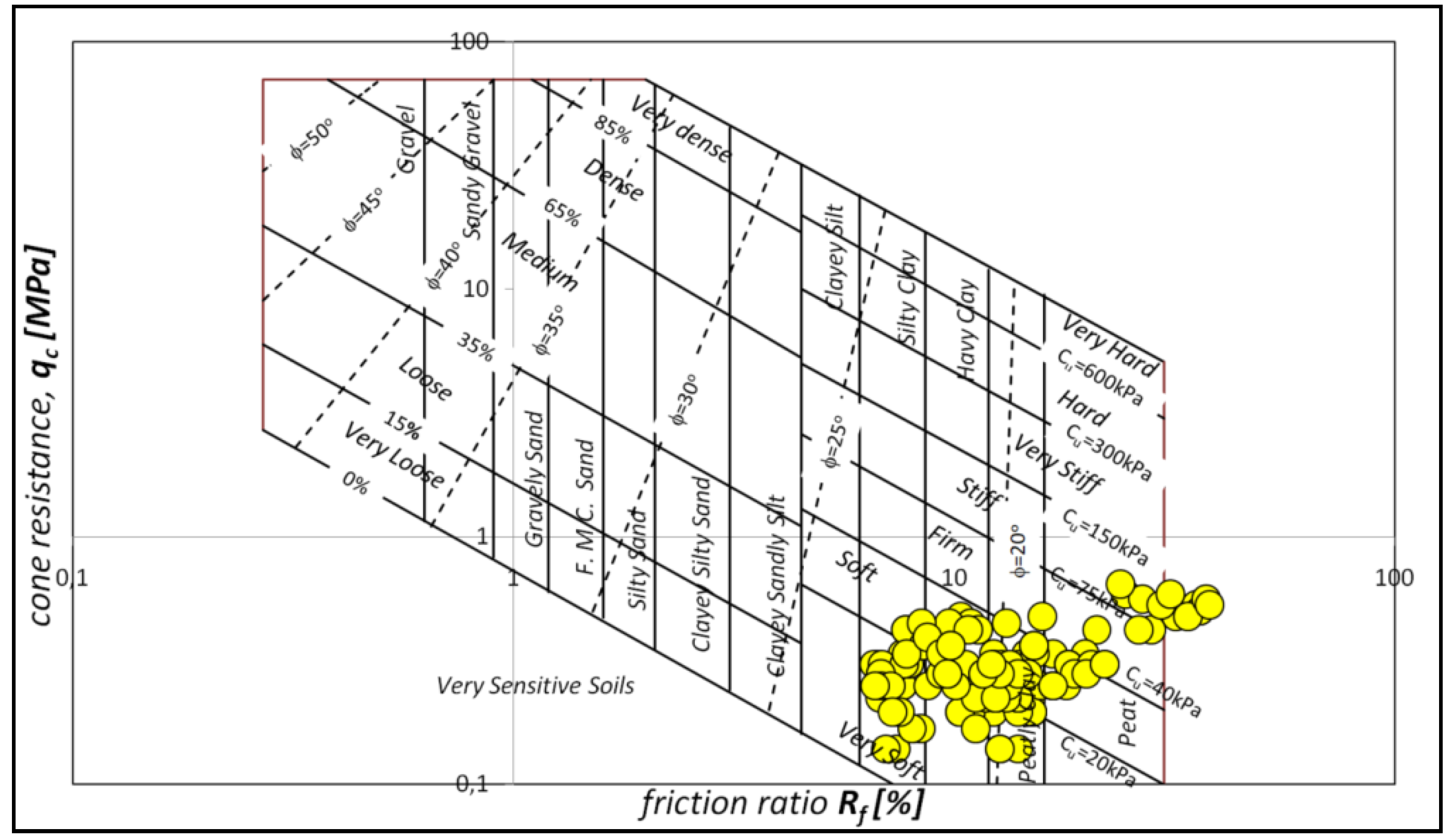
Based on the analysis of the exploratory research carried out in the study area at the Rzeszów site, with the CPTM probe used at a maximum depth 15.4 m below ground level, frequently occurring and varied organic soils were identified in the subsoil. The test results show the values of the cone resistance q_c and sleeve friction f_s, in addition to the friction ratio R_f, which was used for the classification of the organic soil type using known criteria (p.2.1), as presented in the diagrams in Figure 3, Figure 4, Figure 5, Figure 6, Figure 7 and Figure 8.

Existing laboratory research has shown that, in the subsoil, a full spectrum of organic soils are present, from the low to high organic soil, which, due to ambiguous and simplified extant classification criteria [53,54], in comparison to the withdrawn national standard guidelines [55], is currently difficult to exactly define [56,57]. The organic content of the researched soils ranged from ca. 5% to ca. 85%, with a natural water content ranging from ca. 24% to ca. 418% and bulk density from 1.17 kN/m³ to 2.25 kN/m³. The complete results of the index properties of organic soils at the study area at the Rzeszow site are summarized in

Table 1. Index properties of organic soils at the Rzeszow site.

Material	Organic Content LOIT (%)	Water Content W (%)	Bulk Density ρ (t/m3)	Soil Unit Weight γ (kN/m3)	Specific Density ρd (t/m3)	Specific Density ρs (t/m3)
Various organic soils	5.02–84.93	23.52–417.91	1.17–2.25	10.27–19.86	0.23–1.82	1.52–2.59

.

4. Evaluation of the Soil Unit Weight Based on Laboratory Test Results

The next step after performing laboratory tests was to search for the relationships between the dependent (soil unit weight γ_t) and independent variables (natural water content w; organic matter content LOI_T).

The one-factor relationship between the soil unit weight and natural water content is presented and described in the formula in Figure 9a and the organic matter content in Figure 9b. It has been shown that there is a very strong relationship between the variables included, as evidenced by the high value of the coefficient of determination R², for natural water content (0.978) and only slightly lower for organic matter content (0.946). The differences between the values of the soil unit weight, calculated separately for each of the variables, with the value determined in a laboratory, were comparable. In the case of the first variable—natural water content—the max. difference was 21.76%, and for the second variable—soil matter content—the max. difference was 20.46%, in relation to the expected value of the soil unit weight.

Additionally, based on the regression analysis, the relationship between empirically determined values of soil unit weight and leading parameters (natural water content and organic content) was determined and is described by the following formula:

$${\gamma }_t=17,4603+0,0407LO{I}_T-0,0307w$$

(4)

where γ_t is the soil unit weight, LOI_T is the organic content and w is the natural water content.

The differences between the values determined on the basis of laboratory tests and the model determined by the regression method, taking into account two variables, did not exceed 2.95 kN/m³ (22.44%), with the factor R² = 0.797. Variable significance studies (w, LOI_T) were conducted and showed that the variable representing the organic content was not significant. After eliminating the insignificant variable, it was found that the differences between the set value and the expected volume of the soil unit weight were much higher at 3.96 kN/m³ (38.00%), in comparison to the case of the model with two variables. Due to the larger differences and the fact that the model with one explanatory variable was not very representative, the model with two variables was adopted for further analysis. The comparison of the results is presented in Figure 10.

For the analytical estimation of the soil unit weight, personally determined one and two-factor relationships were used; therefore, it was necessary to determine the value of the relative error in the relationships in relation to the values determined empirically in the laboratory.

The maximum and minimum values of relative error were calculated according to Formula (5):

$$RE=\left|\frac{d_p-y_p}{d_p}\right|100\%$$

(5)

where P is number of cases, p = {1,…, P}, d_p is the measured value and y_p is the calculated value.

The comparison carried out for the relationship described earlier indicates a much larger value of the relative error of soil unit weight, which was noted for the one-factor relationship based on organic content (LOI_T), while the lowest, comparable values were obtained for one-factor (w) and two-factor (w, LOI_T) relationships. A summary of the calculated values of relative error (RE) of the soil unit weight is shown in

Table 2. Relative error (RE) of the evaluated soil unit weight of organic soil for use in single and two-factor relationships.

	REγ (w) [%]	REγ (LOIT) [%]	REγ (w; LOIT) [%]
RE MAX	21.76	121.21	22.45
RE MIN	0.07	1.19	0.01

.

The results show that evaluation of the soil unit weight, based only on organic content, is not recommended, but two-factors relationships, based on organic content and natural water content, result in better accuracy and a better way to describe the model.

4.1. Standard Regreesion

The most important task of our analyses is to compare the results of standard regression to the neural network approach in the problem of soil unit mass identification. For this reason, a division of the entire set of 135 measurements into two groups (70%, 30%) was assumed. Ninety-four of them were used as basic data to calculate the parameters of the regression fit function. The remaining 41 were used to test the predictions of the soil unit mass from the regression model with measured values. To determine the statistical evaluation during the analysis, the basic data set was randomly selected 250 times.

Four regression models of one variable were used: the two-parameter linear model (6), three-parameter polynomial model (7), two-parameter power model (8) and four-parameter power model (9).

$$F1\left(x\right)=p_1+p_{2}x$$

(6)

$$F2\left(x\right)=p_1+p_{2}x+p_3{x}^2$$

(7)

$$F3\left(x\right)=p_1{e}^{p_{2}x}$$

(8)

$$F4\left(x\right)=p_1{e}^{p_{2}x}+p_3{e}^{p_{4}x}$$

(9)

Additionally, the next four regression models of the two variables were used: the three-parameter surface model (10), five-parameter surface model (11,12) and eight-parameter surface model (13).

$$F5\left(x,y\right)=p_1+p_{2}x+p_{3}y$$

(10)

$$F6\left(x,y\right)=p_1+p_{2}x+p_{3}y+p_4{x}^2+p_5{x}^{2}y$$

(11)

$$F7\left(x,y\right)=p_1+p_{2}x+p_{3}y+p_4{y}^2+p_{5}x{y}^2$$

(12)

$$F8\left(x,y\right)=p_1+p_{2}x+p_{3}y+p_4{x}^2+p_5{y}^2+p_6{x}^{2}y+p_{7}x{y}^2+p_8{x}^2{y}^2$$

(13)

The goodness of fit was checked using the coefficient of determination (14), mean relative error (15) and mean squared error (16):

$$R^2=1-\frac{{{\displaystyle \sum }}_{p=1}^n{\left(d_p-y_p\right)}^2}{{{\displaystyle \sum }}_{p=1}^n{\left(d_p-{\overline{d}}_p\right)}^2}=\frac{{{\displaystyle \sum }}_{p=1}^n{\left(y_p-{\overline{d}}_p\right)}^2}{{{\displaystyle \sum }}_{p=1}^n{\left(d_p-{\overline{d}}_p\right)}^2}$$

(14)

$$MRE=\frac{1}{n}{\displaystyle \sum }_{p=1}^n\left|\frac{d_p-y_p}{d_p}\right|100\%$$

(15)

$$MSE=\frac{1}{n}{\displaystyle \sum }_{p=1}^n{\left(y_p-d_p\right)}^2$$

(16)

where n is number of cases, $d_p$ is the measured values, $y_p$ is the fitted values (predicted) and ${\overline{d}}_p$ is the mean of the measured values.

The comparison of the median of the goodness of fit obtained for the regression of the one variable model is presented in

Table 3. The goodness of fit for regression of the one variable models.

Soil Parameter		F1		F2		F3		F4
		Base	Test	Base	Test	Base	Test	Base	Test
γt (LOIT)	R2	0.751	0.765	0.911	0.914	0.804	0.814	0.939	0.939
	MRE [%]	7.06	7.05	3.79	3.84	6.42	6.47	2.85	2.90
	MSE	1.664	1.664	0.608	0.608	1.315	1.315	0.413	0.413
γt (w)	R2	0.791	0.802	0.933	0.942	0.840	0.850	0.975	0.976
	MRE [%]	6.38	6.42	3.26	3.12	5.71	5.78	1.80	1.83
	MSE	1.411	1.411	0.450	0.450	1.086	1.086	0.174	0.174

. The median is the most resistant statistic datum and is of central importance in robust statistics. The best model obtained in the analyses was the power model F4, using natural water content. It has 1.83% of the median average relative error for testing the model.

The comparison of the MRE models, included in Table 3 for laboratory data, is presented using box-and-whisker diagrams in Figure 11. On each box, the central mark is the median, the edges of the box are the 25th and 75th percentiles, the whiskers extend to the most extreme data points, which are not considered outliers, and outliers are plotted individually.

Generally, we obtained better results using natural water content.

Table 4. The goodness of fit for the regression of the two variables models.

Soil Parameter		F5		F6		F7		F8
		Base	Test	Base	Test	Base	Test	Base	Test
γt (LOIT, w)	R2	0.798	0.798	0.938	0.936	0.938	0.935	0.939	0.932
	MRE [%]	6.22	6.50	3.19	3.44	3.22	3.51	3.17	3.59
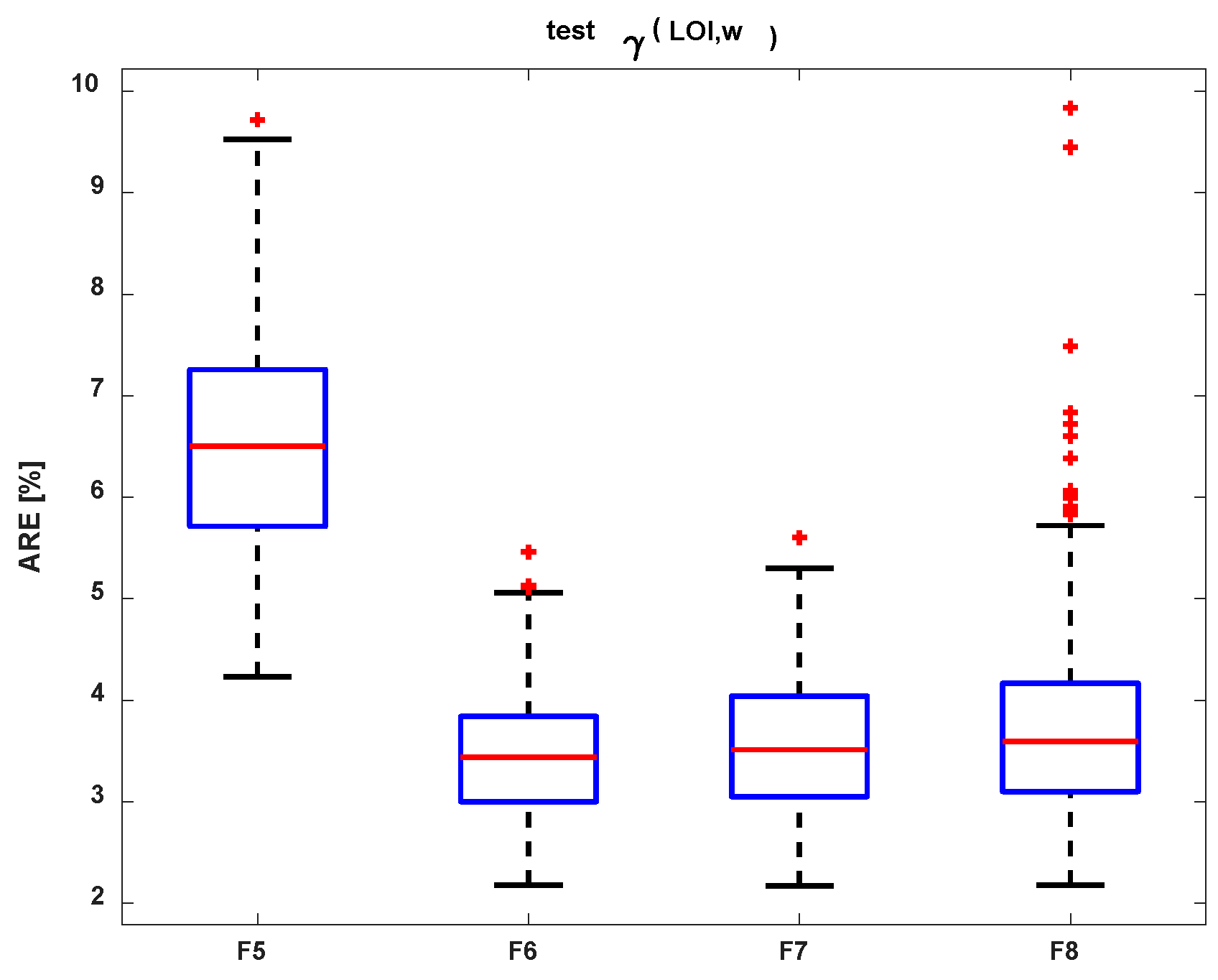
	MSE	1.367	1.423	0.415	0.426	0.416	0.470	0.410	0.484

presents a comparison of the median of the goodness of fit obtained for the two variables regression models (F5–F8). The best result we obtained was for the F6 regression model.

The comparison of the test results from the MRE of models are included in Table 4 for two laboratory parameters (LOI_T, w) and are presented in Figure 12. The model F6 had the least outliers.

Figure 13 shows detailed results from the F6 model with two variables (LOI_T, w). The left-hand plot (Figure 13a), with the blue line, is related to the base data, and the right-hand plot (Figure 13b), with the green line, is related to the test data. The coefficients of determination are very similar.

4.2. Artificial Neural Networks Analysis

Next, we applied a neural regression model. In all the examples, standard multi-layer perception with one hidden layer was applied. In this case, the nets have only one element in the output vector (soil unit weight). The number of hidden neurons is obtained from a cross-correlation procedure. In the calculations, five to eight neurons were used in the hidden layers. Exactly the same pattern divided as that for the standard regression was used to learn and test the networks. The comparison of the median of the goodness of fit, obtained for a few architectures, is presented in

Table 5. The goodness of fit of the ANN models with one input.

Soil Parameter		[1-5-1]		[1-6-1]		[1-7-1]		[1-8-1]
		Learn	Test	Learn	Test	Learn	Test	Learn	Test
γt (LOIT)	R2	0.945	0.948	0.944	0.947	0.945	0.947	0.945	0.947
	MRE [%]	2.70	2.73	2.69	2.76	2.68	2.76	2.64	2.75
	MSE	0.381	0.346	0.380	0.352	0.379	0.341	0.376	0.350
γt (w)	R2	0.976	0.978	0.977	0.979	0.977	0.979	0.977	0.979
	MRE [%]	1.63	1.65	1.62	1.66	1.60	1.67	1.56	1.65
	MSE	0.160	0.146	0.160	0.143	0.159	0.144	0.158	0.144

.

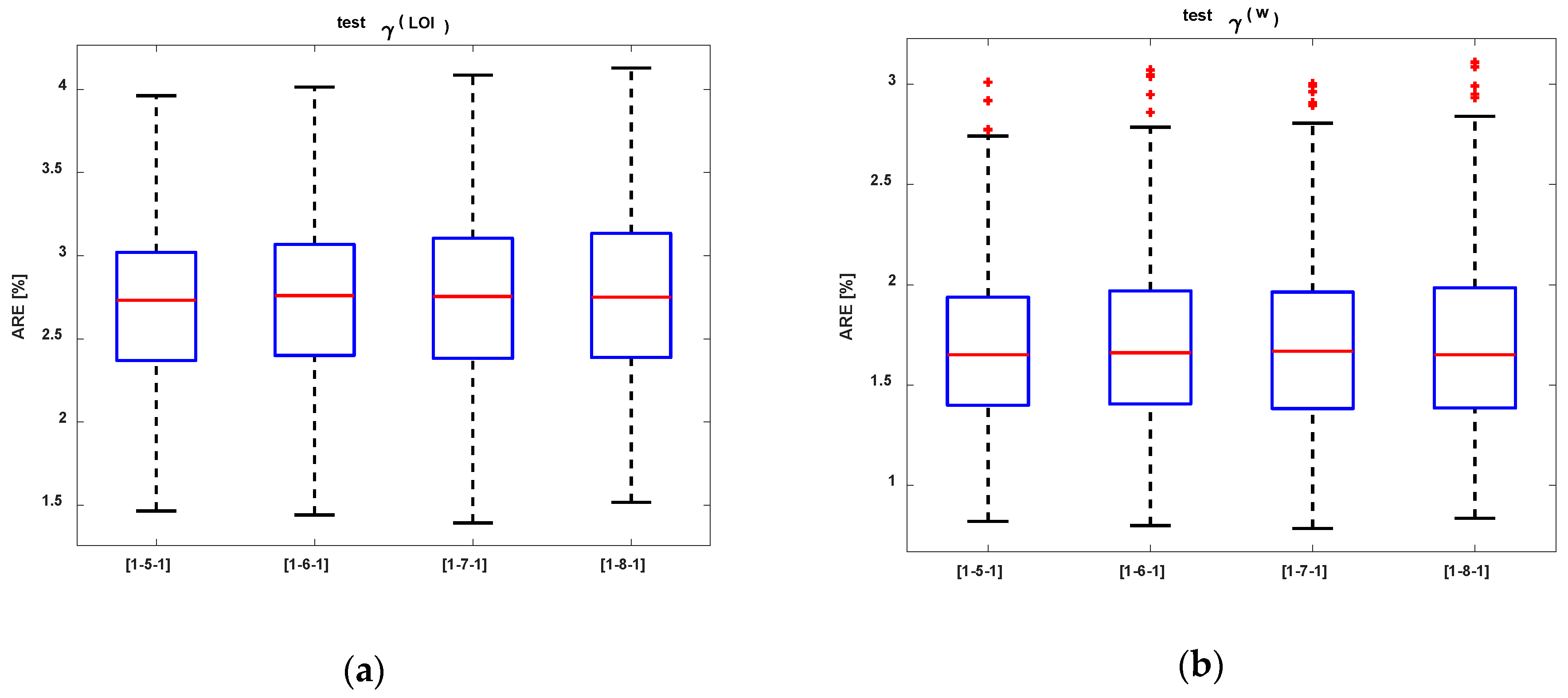
The presented results include the median obtained parameters for one element in the input vector. During the calculation of the values, 20 repetitions of the network training were taken into account for each of the 250 pattern divisions. In this way, 1000 results were finally taken into account. Better prediction was obtained, like that in the standard regression for natural water content, in the input vector. A comparison of the MRE of the nets, included in Table 5, is presented in Figure 14.

In this particular case, the network architecture does not affect the accuracy of approximation. Obtained mean relative errors of testing using organic matter content were in the range of 2.73–2.76%. Respectively, the MRE of testing using natural water content were in the range of 1.65–1.67%. In

Table 6. The goodness of fit of the ANN models with two inputs.

Soil Parameter		[2-5-1]		[2-6-1]		[2-7-1]		[2-8-1]
		Learn	Test	Learn	Test	Learn	Test	Learn	Test
γt (LOIT, w)	R2	0.982	0.986	0.982	0.986	0.982	0.986	0.983	0.986
	MRE [%]	1.39	1.44	1.39	1.42	1.36	1.40	1.36	1.42
	MSE	0.125	0.095	0.125	0.094	0.122	0.093	0.121	0.093

, the comparison of the median result, obtained for the nets with two elements in the input vector, is presented. In that approach, we also obtained a better result, like that in the standard regression with two independent variables. The mean relative errors of testing using two parameters were in the range of 1.40–1.44%.

The comparison test results from the MRE of models, included in Table 6 for two laboratory parameters (LOI_T, w), are presented in Figure 15. There is no clear difference in the results. The obtained results for the two inputs are a little better, which is the opposite case for the nets with one input. The smallest median average relative error test of the ANN was equal to 1.40%.

Figure 16 shows detailed results for the ANN’s prediction of the soil unit weight using two variables (LOI_T, w) in the input vector. Figure 16a shows learning data and Figure 16b shows the test data. The coefficients of determination are very similar.

Generally, the use of neural networks has allowed the soil unit weight values to be predicted based on laboratory tests with very high accuracy. The ANN regression models are slightly better than in the considered regression models. There is no clear difference in the architecture nets used. The best prediction neural networks were determined based on the lowest average relative error.

5. Conclusions

The presented results from the investigation of organic soils allowed for the estimation of the parameters necessary for geotechnical design and soil unit weight, without samples with undisturbed structures. The application of standard regression and neural networks to predict soil unit weight using laboratory tests was possible with acceptable prediction qualities. The maximum median values of the coefficient of determination obtained were equal, respectively, to 0.970 and 0.986. The sampling and preparation laboratory tests were very difficult, time-consuming and expensive. Therefore, the search for cheaper, faster and easier methods to determine soil unit weight in engineering practice is expected. The use of CPTM measurement results using standard regression and ANNs should be verified in the near future.

References

1. Lune, T.; Robertson, P.; Powell, J. Cone Penetration Testing in Geotechnical Practice; CRC Press: London, UK, 1997. [Google Scholar]
2. Mayne, P. Cone Penetration Testing, A Synthesis of Highway Practice, NCHRP Synthesis 368; Transportation Research Board: Washington, DC, USA, 2007. [Google Scholar]
3. Robertson, P.; Cabal, K. Estimating soil unit weight from CPT. In Proceedings of the 2rd International Symposium on Cone Penetration Testing, Huntington Beach, CA, USA, 9–11 May 2010. [Google Scholar]
4. Mayne, P.; Peuchen, J.; Bouwmeester, D. Soil unit weight estimation from CPTs. In Proceedings of the 2rd International Symposium on Cone Penetration Testing, Huntington Beach, CA, USA, 9–11 May 2010; pp. 169–176. [Google Scholar]
5. Cai, G.; Liu, S.; Zhang, T.; Zou, H.; Puppala, A. Evaluation of unit weight from SCPTuin soft marine Jiangsu clay. In Proceedings of the 3rd International Symposium on Cone penetration testing, Las Vegas, NV, USA, 12–14 May 2014; Robertson, K., Cabal, K.I., Eds.; ISSMGE technical Committee: Las Vegas, NV, USA, 2014. [Google Scholar]
6. Lengkeek, H.J.; de Greef, J.; Joosten, S. CPT based unit weight estimation extended to soft organic soils and peat. In Cone Penetration Testing 2018; Hicks, P., Hicks, P., Eds.; Delft University of Technology: Delft, The Netherlands, 2018; pp. 389–395. ISBN 978-1-138-58449-5. [Google Scholar]
7. Straż, G. Estimating soil unit weight from CPT for selected organic soils. In Selected Technical, Economic and Ecological Aspects of Contemporary Construction; Pujer, K., Ed.; Exante Scientific Publisher: Wrocław, Poland, 2016; pp. 63–77. [Google Scholar]
8. Sulewska, M.J. Applying Artificial Neural Networks for analysis of geotechnical problems. Comput. Assist. Methods Eng. Sci. 2011, 18, 230–241. [Google Scholar]
9. Sulewska, M.J. Artificial Neural modeling of compaction characteristics of cohesionless soil. Comput. Assist. Methods Eng. Sci. 2010, 17, 27–40. [Google Scholar]
10. Sulewska, M.J. Artificial Neural Networks in the Evaluation of Non-Cohesive Soil Compaction Parameters; Committee Civil Engineering of the Polish Academy of Sciences: Warsaw, Poland, 2009. [Google Scholar]
11. Sulewska, M.J. About usability of the artificial neural networks in embankment compaction estimation. Inżynieria I Budownictwo 2006, 6, 337–338. [Google Scholar]
12. Sulewska, M.J. Prediction Models for Minimum and Maximum Dry Density of Non-Cohesive Soils. Pol. J. Environ. Stud. 2010, 19, 797–804. [Google Scholar]
13. Lechowicz, Z.; Fukue, M.; Rabarijoely, S.; Sulewska, M.J. Evaluation of the Undrained Shear Strength of Organic Soils from a Dilatometer Test Using Artificial Neural Networks. Appl. Sci. 2018, 8, 1395. [Google Scholar] [CrossRef] [Green Version]
14. Ochmański, M.; Bzówka, J. Selected examples of the use of artificial neural networks in geotechnics. Civ. Environ. Eng. 2013, 4, 287–294. [Google Scholar]
15. Ochmański, M.; Bzówka, J. Back analysis of SCL tunnels based on Artificial Neural Network. Archit. Civ. Eng. Environ. 2012, 3, 73–81. [Google Scholar]
16. Ochmański, M. The use of artificial neural networks for influence analysis of selected parameters on the jet grouting columns diameters. In Proceedings of the XIII Scientific Conference for Civil Engineering Ph.D. Students, Szczyrk, Poland, 12–13 September 2013. [Google Scholar]
17. Borowiec, A.; Wilk, K. Prediction of consistency parameters of fen soils by neural networks. Comput. Assist. Methods Eng. Sci. 2014, 21, 67–75. [Google Scholar]
18. Klos, M.; Sulewska, M.J.; Waszczyszyn, Z. Neural identification of compaction characteristics for granular soils. Comput. Assist. Methods Eng. Sci. 2011, 18, 265–273. [Google Scholar]
19. Kłos, M.; Waszczyszyn, Z. Prediction of Compaction Characteristics of Granular Soils by Neural Networks. Artif. Neural Netw. 2010, 42–45. [Google Scholar] [CrossRef]
20. Wrzesiński, G.; Sulewska, M.J.; Lechowicz, Z. Evaluation of the Change in Undrained Shear Strength in Cohesive Soils due to Principal Stress Rotation Using an Artificial Neural Network. Appl. Sci. 2018, 8, 781. [Google Scholar] [CrossRef] [Green Version]
21. Zabielska-Adamska, K.; Sulewska, M.J. Ann-based modelling of fly ash compaction curve. Arch. Civ. Eng. 2012, 1, 57–69. [Google Scholar] [CrossRef] [Green Version]
22. Zhiming, C.H.; Guotao, M.; Ye, Z.; Yanjie, Z.; Hengyang, H. The application of artificial neural network in geotechnical engineering. In Proceedings of the 2018 International Conference on Civil and Hydraulic Engineering (IConCHE 2018), Qingdao, China, 23–25 November 2018; IOP Publishing: Bristol, UK, 2018. [Google Scholar] [CrossRef]
23. Shahin, M.; Jaksa, M.; Maier, H. Artificial neural network applications in geotechnical engineering. Aust. Geomech. 2001, 36, 49–62. [Google Scholar]
24. Cal, Y. Soil classification by neural-network. Adv. Eng. Softw. 1995, 22, 95–97. [Google Scholar] [CrossRef]
25. Ferentinou, M.; Hasiotis, T. Application of computational intelligence tools for the analysis of marine geotechnical properties in the head of Zakynthos canyon. Greece Comput. Geosci. 2012, 40, 166–174. [Google Scholar] [CrossRef]
26. Ferentinou, M.; Sakellariou, M. Computational intelligence tools for the prediction of slope performance. Comput. Geotech. 2007, 34, 362–384. [Google Scholar] [CrossRef]
27. Wang, Z.; Li, Y. Correction of soil parameters in calculation of embankment settlement using a BP network back-analysis model. Eng. Geol. 2007, 91, 168–177. [Google Scholar] [CrossRef]
28. Ylmaz, I.; Yuksek, A. An example of artificial neural network (ANN) application for indirect estimation of rock parameters. Rock Mech. Rock Eng. 2008, 41, 781–795. [Google Scholar] [CrossRef]
29. Nawari, N.; Liang, R.; Nusairat, J. Artificial intelligence techniques for the design and analysis of deep foundations. Electron. J. Geotech. Eng. 1999, 4, 1–21. [Google Scholar]
30. Goh, A. Empirical design in geotechnics using neural networks. Geotechnique 1995, 45, 709–714. [Google Scholar] [CrossRef]
31. Penumadu, D.; Jean-Lou, C. Geomaterial modeling using artificial neural networks. In Artificial Neural Networks for Civil Engineers: Fundamentals and Applications; ASCE: Reston, WV, USA, 1997; pp. 160–184. [Google Scholar]
32. PN-EN ISO 22476-12:2009. Geotechnical Investigation and Testing—Field Testing—Part 12: Mechanical Cone Penetration Test; ISO: Geneva, Switzerland, 2009. [Google Scholar]
33. Młynarek, Z.; Tschuschke, W.; Wierzbicki, J. Geotechnics in construction and transport. In Proceedings of the 11th National Conference on Soil Mechanics and Foundation Engineering, Gdańsk, Poland, 25–27 June 1997; pp. 119–126. [Google Scholar]
34. Douglas, B.J.; Olsen, R.S. Soil classification using electric cone penetrometer. American Society of Civil Engineers, ASCE. In Proceedings of the Conference on Cone Penetration Testing and Experience, St. Louis, MI, USA, 26–30 October 1981; pp. 209–227. [Google Scholar]
35. Schmertmann, J.H. Guidelines for Cone Test, Performance, and Design; Report FHWA-TS-78209; Federal Highway Administration: Washington, DC, USA, 1978; p. 145.
36. Eslami, A.; Fellenius, B.H. CPT and CPTu data for soil profile interpretation: Review of method sand proposed new approach. Iran. J. Sci. Technol. 2004, 28, 71–86. [Google Scholar]
37. Robertson, P.K.; Capanella, R.G. Interpretation of cone penetration testsPart II (clay). Can. Geotech. J. 1983, 20, 734–745. [Google Scholar] [CrossRef]
38. Searle, I.W. The interpretation of Begemann friction jacket cone results to give soil types and design parameters. In Proceedings of the 7th European Conference on Soil Mechanics and Foundation Engineering, ECSMFE, Brighton, UK, 1–6 September 1979; pp. 2265–2270. [Google Scholar]
39. PN-EN ISO 17892-1. Geotechnical Investigation and Testing—Laboratory Testing of Soil—Part 1: Determination of Water Content; ISO: Geneva, Switzerland, 2007. [Google Scholar]
40. PN-EN 1997-2: 2007. Eurocode 7: Geotechnical Design—Part 1: Ground Investigation and Testing; ISO: Geneva, Switzerland, 2007. [Google Scholar]
41. PN-B-04481: 1998. Building Soils. Laboratory Tests; Polish Standard: Warsaw, Poland, 1998. [Google Scholar]
42. Marut, M.; Straż, G. Verification of standard guidelines for organic matter content determination in organic soils by the loss on ignition method. Geol. Rev. 2016, 64, 918–924. [Google Scholar]
43. Heiri, O.; Lotter, A.F.; Lemcke, G. Loss on ignition as a method for estimating organic and carbonate content in sediments: Reproducibility and comparability of results. J. Paleolimnol. 2001, 25, 101–110. [Google Scholar] [CrossRef]
44. PN-EN ISO 17892-2:2014. Geotechnical Investigation and Testing—Laboratory Testing of Soil—Part 2: Determination of Bulk Density (ISO 17892-2:2014); ISO: Geneva, Switzerland, 2014. [Google Scholar]
45. Geotech, Z.O.O. Department of Geological Services Design and Construction and the Environment, Geological and Engineering Geological Conditions for Recognition—Engineering for the Construction of Multi-Storey Building at UL; Witolda in Rzeszów: Rzeszow, Poland, 2010. [Google Scholar]
46. Haykin, S.O. Neural Networks and Learning Machines, 3rd ed.; Pearson Education: Upper Saddle River, NJ, USA, 2009; p. 798. [Google Scholar] [CrossRef]
47. Hagan, M.T.; Demuth, H.B.; Beale, M.H. Neural Network Design; PWS Publishing: Boston, MA, USA, 1996. [Google Scholar]
48. Marquardt, D. An Algorithm for Least-Squares Estimation of Nonlinear Parameters. SIAM J. Appl. Math. 1963, 11, 431–441. [Google Scholar] [CrossRef]
49. Hagan, M.T.; Menhaj, M. Training feed-forward networks with the Marquardt algorithm. IEEE Trans. Neural Netw. 1994, 5, 989–993. [Google Scholar] [CrossRef]
50. Dennis, J.E.; Schnabel, R.B. Numerical Methods for Unconstrained Optimization and Nonlinear Equations; Prentice-Hall: Englewood Cliffs, NJ, USA, 1983. [Google Scholar]
51. MacKay, D.J.C. Bayesian interpolation. Neural Comput. 1992, 4, 415–447. [Google Scholar] [CrossRef]
52. Beale, M.H.; Hagan, M.T.; Demuth, H.B. Neural Network ToolboxUser’s Guide; TheMathWorks: Natick, MA, USA, 2010. [Google Scholar]
53. PN EN-ISO 14688-1:2018. Geotechnical Investigations and Testing—IDENTIFICATION and Classification of —Part 1: Identification and Description; ISO: Geneva, Switzerland, 2018. [Google Scholar]
54. PN EN-ISO 14688-1:2018. Geotechnical Investigations and Testing—Identification and Classification of —Part 2: Principles for a Classification; ISO: Geneva, Switzerland, 2018. [Google Scholar]
55. PN-B-02480: 1986. Building Soils. Nomenclature, Symbols, Classification and Description of Soils; Polish Standard: Warsaw, Poland, 1986. [Google Scholar]
56. Straż, G. Identification of local organic soils based on cone penetration test results. Civ. Eng. Archit. 2014, 13, 49–56. [Google Scholar]
57. Straż, G. Identification, marking and classification methods of organic soils according to Eurocode 7 and related standards. Scientific Review—Engineering and Environmental Sciences. Sci. Rev. Eng. Env. Sci. 2018, 27. [Google Scholar] [CrossRef] [Green Version]
Figure 1. Selected cross-section of the local subsoil based on CPTM probes at the Rzeszow site. CPTM: cone penetration test.
Applsci 10 02261 g001
Figure 2. Diagram of the artificial neural network.
Applsci 10 02261 g002
Figure 3. Diagrams present the identification of organic soils based on Cone Penetration Tests (CPTM), according to the propositions of Robertson’s nomogram and adapted to Polish conditions.
Applsci 10 02261 g003
Figure 4. Diagrams present the identification of organic soils based on CPTM tests, according to the propositions of Olsen’s nomogram.
Applsci 10 02261 g004
Figure 5. Diagrams present the identification of organic soils based on CPTM tests, according to the propositions of Schmertmann’s nomogram.
Applsci 10 02261 g005
Figure 6. Diagrams present the identification of organic soils based on CPTM tests, according to the propositions of Schmertmann’s nomogram and taking into account Bergman’s criterion.
Applsci 10 02261 g006
Figure 7. Diagrams present the identification of organic soils based on CPTM tests, according to the propositions of Robertson and Capanella’s nomogram.
Applsci 10 02261 g007
Figure 8. Diagrams present the identification of organic soils based on CPTM tests, according to the propositions of Searle’s nomogram.
Applsci 10 02261 g008
Figure 9. The value of the soil unit weight estimated from laboratory tests was in reference to (a) natural water content and (b) organic matter content.
Applsci 10 02261 g009
Figure 10. Comparison between measured values of soil unit weight and the values expected, based on regression analysis, including the model with (a) two independent variables (w; LOIT) and (b) one independent variable (w).
Applsci 10 02261 g010
Figure 11. Comparison of the MRE tested models (F1–F4): (a) LOIT and (b) w.
Applsci 10 02261 g011
Figure 12. Comparison of the MRE tested models (F5–F8).
Applsci 10 02261 g012
Figure 13. Regression of the F6 model of soil unit weight (LOIT, w): (a) base data and (b) test data.
Applsci 10 02261 g013
Figure 14. Comparison of the MRE of the nets with one element in the input vector: (a) LOIT and (b) w.
Applsci 10 02261 g014
Figure 15. Comparison of the MRE of the nets with two elements in the input vector.
Applsci 10 02261 g015
Figure 16. Regression of the ANN prediction of soil unit weight (LOIT, w): (a) learn data and (b) test data.
Applsci 10 02261 g016