Damage Identification Based on Adding Mass for Liquid–Solid Coupling Structures

Abstract

Damage identification for liquid–solid coupling structures remains a challenging topic due to the influence of liquid and the limitation of experimental conditions. Therefore, the adding mass method for damage identification is employed in this study. Adding mass to structures is an effective method for damage identification, as it can increase not only the experimental data but also the sensitivity of experimental modes to local damage. First, the fundamental theory of the adding mass method for damage identification is introduced. After that, the method of equating the liquid to the attached mass is proposed by considering the liquid–solid coupling. Finally, the effectiveness and reliability of damage identification, based on adding mass for liquid–solid coupling structures, are verified through experiments of a submerged cantilever beam and liquid storage tank.

1. Introduction

In recent years, with the development of civil engineering, the number of complex structures and large-scale structures increases gradually. To ensure the safety of structures, structural health monitoring (SHM) became a very important research topic and many effective SHM methods were developed [1,2,3,4,5]. Damage identification methods [6,7,8,9,10,11,12] can provide critical theoretical foundations for SHM. Because of the rapid development of sensor techniques and experimental protocols, damage identification methods, based on the structural dynamic response, have been widely studied and applied, including the time-domain response-based methods and the modal response-based methods. Methods based on time-domain response mainly utilize signal processing techniques to identify structural damages. These techniques include wavelet analysis, empirical mode decomposition, etc. Fitzgerald et al. [13] studied bridge scour based on analyzing bogie acceleration measurements using Continuous Wavelet Transform, and the results showed that bridge stiffness was locally reduced. Sadhu et al. [14] detected the structural damages through time-domain responses, using Cauchy continuous wavelet transform. Dos Santos et al. [15] analyzed the influence of wavelet coefficient, the selected modes, and the types of rotation field on damage identification through wavelet post-processing of the modal rotation field. Lofrano et al. [16] proposed a new damage index with orthogonal empirical mode decomposition to identify the damages of structures. The validity of this approach was verified on two structural models. The methods based on modal responses are used to analyze the structural physical parameters using the modal changes before and after the damages. Then the damage location and degree can be determined. Ozdagli et al. [17] proposed a new system to reconstruct structural features for damage detection, which are similar to the original features, based on the natural frequencies and mode shapes of the undamaged structure. Nguyen et al. [18] analyzed the ratio of the eigenvalue and the modal strain energy to identify the damage of complex structures. Garcia-Macias et al. [19] studied three different structures by analyzing the propagation of waves. Zai et al. [20] discussed many damage identification methods based on structural parameters, including natural frequencies and mode shapes. In general, modes are the structural characteristic parameters independent of the extra loads. Moreover, they are highly stable and insensitive to noise. These characteristics can ensure the reliability and accuracy of the damage identification results. Hence, the damage identification based on modal responses is adopted in this work.

There are many difficulties in large and complex structures damage identifications, such as complex monitoring environment and limited installation of sensors. In this case, the amount of measurements is less and often insufficient with a large number of low-order modes. Furthermore, the local damage does not affect the whole structure. Therefore, adding mass to the structures or increasing the structural stiffness can significantly boost the experimental information and improve the sensitivity of the experimental modes to local damages. Nalitolela et al. [21] constructed a new structure by adding stiffness to the original structure and acquired new frequency response functions based on original structural response information. Cha et al. [22] modified the mass matrix and stiffness matrix by considering both the vibration modes of additional mass structure and initial structure, to improve the consistency between analytical modes and modal survey. Dems et al. [23] attached loads, supports, or masses to plate and frame structures to control the difference between experimental data and numerical predictions, and improved sensitivity of identification. Dinh et al. [24] identified the mass, damping coefficient, and stiffness of structures based on the correlation between the structural modal information and additional masses. Rajendran et al. [25] attached a mass to different locations of a composite plate structure to change the dynamic characteristics. This allowed us to obtain the rotational bending mode shapes to identify damage. Fanning et al. [26] developed a method to determine the additional mass by a linear response function and the correlation analysis model of the structure. Rajendran et al. [27] studied the identification and location of additional mass in beams and the influence of additional mass on the rotational freedom of the beam. Kołakowski et al. [28] used the Virtual Distortion Method to assess truss structural strength and summarized the application of the method in dynamics and statics, and so on. Hou et al. [29] identified the damages of a plane frame by analyzing the frequencies of the structure with additional virtual mass and real structure precisely. Hou et al. [30] combined Bayesian and adding virtual mass method to identify structural damage: this approach was proven. As the adding mass method is convenient for operation in practice, and the measured data is often highly reliable, the same approach is adopted in this study to obtain the structural response information.

Due to the vibration coupling between liquid and solid, the vibration mechanism is complicated for structures immersed in liquids, which increases the difficulty of damage identification. Ellis et al. [31] introduced the model methods and results of the mechanical solid–liquid coupling containing outer slip and inner slip. Zou et al. [32] proposed the water mass and analyzed the dynamic responses of the conical columns in water. Wang et al. [33] derived the solid–liquid coupling vibration equation in the pipe and discussed the influence of solid and liquid dynamic characteristics on natural frequencies. Paik et al. [34] calculated the load of liquid on the hull surface by two coupling methods, considering the ship as elastic. Moiseev et al. [35] computed the modal information of the liquid oscillations in a spherical container by the singularity method. Forouzan et al. [36] coupled the fluid loading and structural responses by a new hybrid simulation technique to determine the interaction between tsunami waves and structures. Li et al. [37] conducted some dynamic tests to study the inertia coefficient and additional hydrodynamic mass, and developed a calculation method. For considering the influence of the liquid–solid coupling vibration on structures, the attached fluid mass method is adopted. The force exerted by the liquid on structures is equivalent to the additional mass effect produced by solid vibration.

This paper is structured as follows. First, the basic theory of adding mass method for damage identification is introduced. Then, considering the liquid–solid coupling, the approach of equaling the liquid to the attached fluid mass is proposed. Finally, the effectiveness and reliability of the proposed method are verified by experiments of a submerged cantilever beam and liquid storage tank.

2. Damage Identification Based on the Adding Mass Method

For submerged structures, it is often a challenge to locate the measuring points due to the influence of liquid. Moreover, structural modes are not sensitive to local damage, which becomes even more complicated for coupling analyses. The adding mass method can overcome these difficulties to some extent. More positions additional masses are added at, more modal information can be obtained, which can lead to more accurate damage identification. Therefore, the adding mass method is employed in this work to identify the damage of submerged structures. A cantilever beam is taken as an example (see Figure 1), the structure is divided into $n$ substructures, which means that the additional mass can take one of the $n$ positions. The global structure is denoted as $S_i$, which refers to the structure with the mass added to the $i$-th substructure. Dynamic experiments are conducted on the structure $S_i$. It is assumed that the first $k$ natural frequencies of the structure can be obtained noted as ${\omega }_i=\left\{{\omega }_{1i},{\omega }_{2i},\dots ,{\omega }_{ki}\right\}$, where ${\omega }_{ji}$ represents the $j$-th natural frequency of the structure with the additional mass added to the $i$-th substructure. From the first to the $n$-th substructure, the total natural frequency matrix can be noted as $\overline{\omega }=\left\{{\omega }_1,{\omega }_2,\dots ,{\omega }_i,\dots ,{\omega }_n\right\}$.

The additional mass can change the dynamic characteristics of the structure, and structural modes can also vary depending on the location of the additional mass. Generally, larger additional masses can lead to greater changes in structural responses. This results in higher effects on the structural dynamic characteristics and local sensitivity. In these circumstances, the same order mode is irrelevant, and the accuracy of damage identification is improved. However, if the additional mass is too large, it may cause difficulty for experiment operation or even structural collapse. If the additional mass is too small, the sensitivity is low, and the effect of additional mass may not be observed. Therefore, the appropriate additional mass is selected according to the relative sensitivity of the natural frequency $R_{ji,l}\left(\mu ,m\right)$ (see Equation (1)), which is calculated by the FE model. The optimal additional mass is determined using the undamaged structure with the damage factor $\mu =1$. Finally, the mass $m$ is modified to achieve the optimal value of $R_{ji,l}\left(\mu ,m\right)$.

$$R_{ji,l}\left(\mu ,m\right)=\frac{\partial {\omega }_{ji}\left(\mu ,m\right)}{{\omega }_{ji}\left(\mu ,m\right)\partial {\mu }_l}=\frac{{\mathsf{\Psi }}_{\mathrm{ji}}^{\mathrm{T}}\left(\mu ,m\right)K_l{\mathsf{\Psi }}_{\mathrm{ji}}\left(\mu ,m\right)}{2{\omega }_{ji}{}^2\left(\mu ,m\right)},$$

(1)

where $R_{ji,l}$ is the relative sensitivity of the $j$-th order natural frequency of the $l$-th substructure, with the additional mass at the i-th position; ${\omega }_{ji}$ and ${\Psi }_{ji}$ are the $j$-th order natural frequency and mode shape of the damaged structure $S_i$; $K_l$ is the undamaged stiffness matrix of the $l$-th substructure; and ${\mu }_l$ is the ratio of stiffness after and before the damage of the $l$-th substructure.

In summary, the steps of the additional mass method include: (1) successively attaching the selected appropriate mass to each substructure of the structure to build new structures, (2) obtaining the natural frequencies information of each new structure by dynamic experiments, (3) using the obtained frequencies to identify structural damage.

3. Attached Fluid Mass Method Considering Liquid–Solid Coupling

Structures in the liquid environment can be influenced by liquid–solid coupling, and the natural frequencies of the structure are changed accordingly. To accurately identify the damage, it is necessary to calculate the modal information of the liquid–solid coupling structures. The equation of structural motion based on liquid–solid coupling is

$$M\ddot{x}+C\dot{x}+Kx=F_s+F_Q,$$

(2)

where $M$, $C$, and $K$ are the mass, damping, and stiffness matrices of the structure, respectively; $F_s$ is the external load;$x$ is the displacement of the structure; and $F_Q$ is the additional hydrodynamic pressure exerted by the liquid on the structure.

According to the fluid FE, the function of the flow field can be arranged into a typical finite element formulation as Equation (3). When the element’s function takes the stationary value of node pressure, the following formula (Equation (4)) can be obtained.

$${\mathsf{\Pi }}_e=\frac{1}{2}{q}^T{H}_{e}q-q^T{F}_e$$

(3)

$$F_e=H_{e}q,$$

(4)

where $H_e$ is equivalent to the stiffness matrix of the structure,$q$ is nodal displacement, $F_e$ is a nodal load. According to the structure FE, the equation of additional hydrodynamic pressure can be acquired as

$$F_Q=M_p\ddot{x},$$

(5)

where $M_p$ is the attached fluid mass matrix, which represents the additional pressure of fluid caused by the vibration acceleration of the structure on the contact surface. Its specific calculation formula can be found in Equations (6) and (7). The detailed derivation of the attached fluid mass (see Equation (6)) is available in Ref. [38].

$$M_p={\displaystyle \sum }_{k=1}^{S_E}{A}_k^T{L}_k{A}_k{H}_N^{-1}{B}_N$$

(6)

$$\{\begin{array}{c}{L}_k=\int N_S^T{N}_{S}dS\\ H_N=H_{nn}-H_{nv}{H}_{vv}^{-1}{H}_{vn}\\ H_e=\int \frac{\partial N^T}{\partial x}\frac{\partial N}{\partial x}+\frac{\partial N^T}{\partial y}\frac{\partial N}{\partial y}+\frac{\partial N^T}{\partial z}\frac{\partial N}{\partial z}dV\\ B_N=\int N^T\xi N_{S}dS\end{array},$$

(7)

where $A_k$ is the position sequence matrix to extract the node hydrodynamic pressure matrix of an element from the hydrodynamic pressure matrix of all contact surface nodes; $N_S$ is the interpolation function of the normal displacement on the contact surface;$S_E$ is the number of fluid elements in contact with the structure;$N$ is the interpolation function of the hydrodynamic pressure at fluid element nodes; $\xi$ is the unitary surface mass of the fluid.

Substituting Equation (5) into Equation (2), the new equation of structure motion is obtained:

$$\left(M+M_p\right)\ddot{x}+C\dot{x}+Kx=F_s,$$

(8)

The dynamic characteristics of the structure influenced by liquid–solid coupling can be analyzed by Equation (8), and the structural modal information can also be calculated accordingly.

4. Damage Identification Experiment of a Submerged Cantilever Steel Beam

In this section, the additional mass method for damage identification is verified by performing an experiment on a submerged cantilever steel beam. As the cantilever beam is submerged in water, it is highly demanding for the sensor type and experimental conditions when the experiment is conducted underwater. The method of adding mass to the cantilever beam is adopted to address the limitations of the experimental conditions. Mass is added at different positions to construct different structures, thereby increasing the amounts of experimental data and improving the accuracy of damage identification.

4.1. Beam Model

The experimental model of the cantilever steel beam, as shown in Figure 2, was 1 m in length, 0.08 m in width, and 0.006 m in height. The cantilever beam was made of steel, whose Young’s is 210$\mathrm{GPa}$ and mass density is 7850$\mathrm{kg}/{\mathrm{m}}^3$. The beam model was rigidly connected to the base by bolts.

The FE model of the cantilever steel beam is established by the beam element in MATLAB, which was divided into 10 substructures, each of which consists of two elements. There were 20 elements and 21 nodes in total.

4.2. Experimental Devices and Process

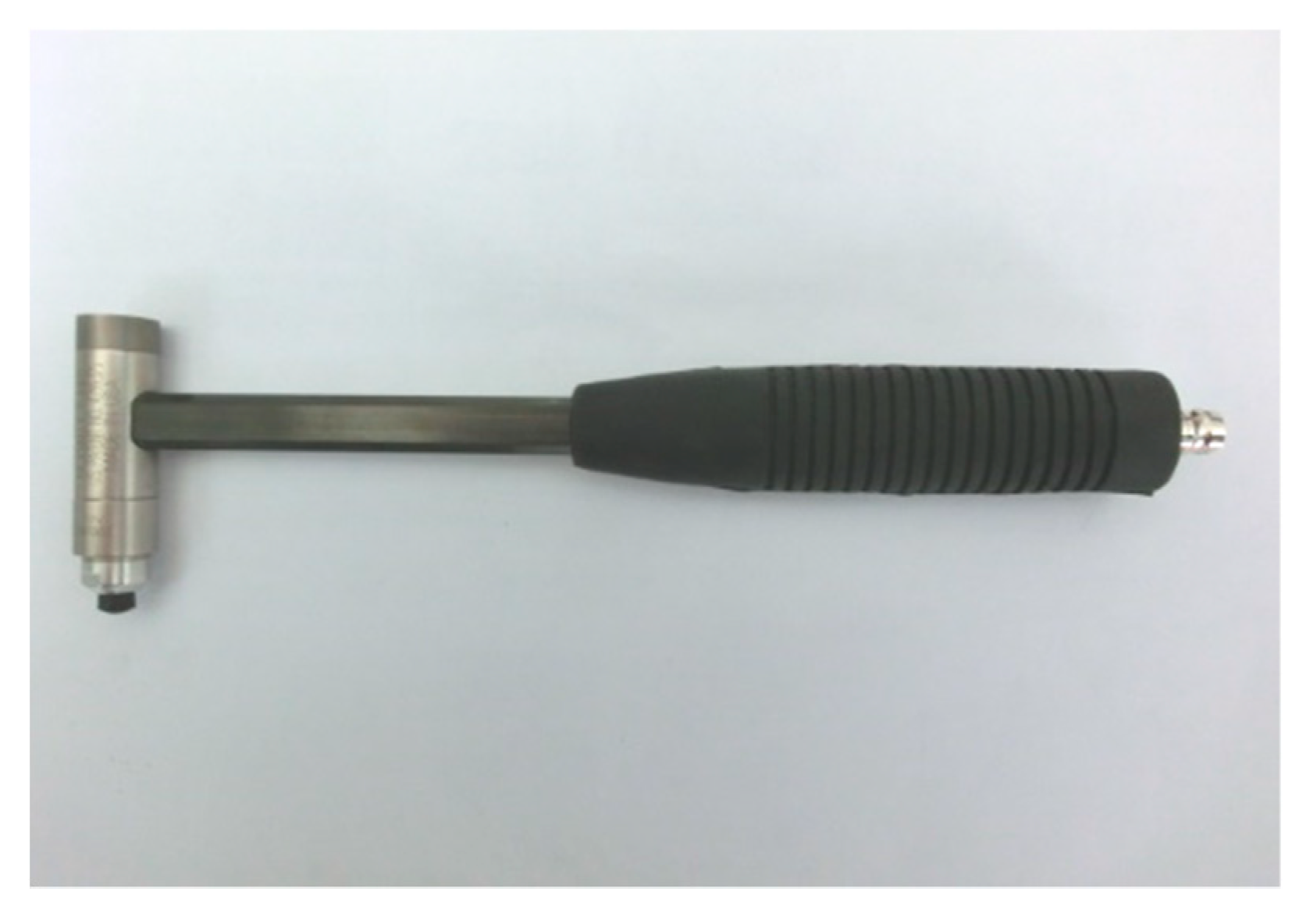
The experimental devices included a modal hammer (see Figure 3 ), which was used to measure the load. An acceleration sensor (see Figure 4), which was used to measure the structural acceleration responses. The type of acceleration sensor is 333B50SNLW52869, and the sensitivity is 992$\mathrm{V}/\mathrm{g}$. The mass of the sensor is 8.2$\mathrm{g},$ and the sampling frequency is 10,000$\mathrm{Hz}$. The signal acquisition unit (see Figure 5) and the signal processing is carried out by MATLAB program.

The experimental process of the cantilever steel beam is as followed.

(1) Put the cantilever beam in the tank and add water into the tank to a certain height.

(2) Put the acceleration sensor on the top of the cantilever beam.

(3) Attach mass to the first substructure by a magnet and knock the top of the beam to obtain acceleration responses.

(4) Move the mass to the next substructure and repeat the same excitation and measurement. The experiment is not completed until all substructures are tested.

4.3. Influence of Immersion Depth on the Natural Frequency of the Cantilever Beam

In order to assess the effect of immersion depth on the natural frequencies of the cantilever beam, the dynamic experiment is carried out for an undamaged cantilever beam under the water in a tank of 0.8 m height (see Figure 6). The immersion depths of the cantilever beam are 0 m, 0.2 m, 0.4 m, 0.6 m, and 0.8 m. Acceleration responses are measured by knocking the top of the cantilever beam. When the mass is attached at the top substructure, and the immersion depth is 0.4 m, the corresponding time-domain acceleration response of the beam is shown in Figure 7. Then, the fast Fourier transform is used to transform measured acceleration responses. Natural frequencies can be obtained by extracting the peak of the frequency spectrum. The natural frequencies of the intact cantilever beam under different immersion depths measured experimentally are listed in

Table 1. First natural frequencies (Hz) of the submerged cantilever beam.

Natural Frequencies		1	2	3	4
0 m	Experiment	5.18	32.58	84.98	167.76
	Theory	5.32	31.97	83.23	171.74
0.2 m	Experiment	5.12	33.45	81.73	164.89
	Theory	5.01	31.20	85.34	163.61
0.4 m	Experiment	4.42	24.74	73.90	162.23
	Theory	4.66	25.75	76.78	157.48
0.6 m	Experiment	4.28	21.44	68.74	152.64
	Theory	4.34	22.36	71.74	148.75
0.8 m	Experiment	4.07	18.99	64.76	146.87
	Theory	4.17	20.86	63.66	145.71

. The FE model of the undamaged submerged cantilever beam can be developed using the adding mass method with the liquid–solid coupling. The theoretical natural frequencies of the beam under different immersion depths are shown in Table 1. Mode shapes of the FE model can be calculated, and the first two shapes of the cantilever beam with 0.4 m immersion depth can be seen in Figure 8.

It can be seen from Table 1 that the first four theoretical and experimental natural frequencies of the submerged beam decrease with the increase of the immersion depth. This means that water can restrain the vibration of the cantilever beam. Meanwhile, the theoretical natural frequencies of the submerged beam are close to the experimental ones, which demonstrates the validity of the experiment when water is used as the attached fluid mass in this work.

4.4. Damage Identification

4.4.1. Damage Scenario

There are two damage scenarios for the cantilever beam, single damage and multiple damages. For single damage, the substructure 9 is damaged, and the stiffness is decreased to 50%; for multiple damages, the substructures 6 and 9 are damaged, and the stiffness of the two substructures is reduced to 50%. In experiments, single damage is simulated by making incisions with 2 cm in length, 0.6 cm in-depth, 1 mm in width, and 1 cm on both sides of the inward of the substructure 9 (see Figure 9). The same incisions in substructures 6 and 9 are made in order to simulate the multiple damages. The immersion depths considered in this study are 0 m, 0.2 m, 0.4 m, 0.6 m, and 0.8 m, respectively.

4.4.2. Determination of the Additional Mass

To improve the accuracy of damage identification, the additional mass that leads to higher sensitivity frequencies of the cantilever beam is selected, according to Section 2. Under different water depth conditions, each substructure is added with mass ranging from 0 $\mathrm{kg}$ to 2 $\mathrm{kg}$. The relative sensitivity of the first four frequencies of the 10 substructures is calculated. When the immersion depth is 0.4 m, the frequency relative sensitivity curves of substructure 7 are shown in Figure 10. The “frequency sensitivity” in Figure 10 is the relative sensitivity of the natural frequency $R_{ji,l}\left(\mu ,m\right)$, which is calculated by Equation (1).

Figure 10 shows that the relative sensitivity of the first frequency decreases with the increase of the mass value; the relative sensitivity of the second and third frequencies increase as the mass value increases; the relative sensitivity of the fourth frequency of substructure 7 remains stable when the additional mass value varies. Furthermore, when the additional mass is 0.3 kg, the relative sensitivity of the first frequency decreases 2%, while the relative sensitivity of second and third frequencies increases by 10%. Overall, 0.3 kg additional mass improves the sensitivity of frequencies and avoids the structural damage caused by excessive mass. Based on these relative sensitivity curves of the 10 substructures, the additional mass is determined to be 0.3 kg when the immersion depth is 0.4 m.

4.4.3. Damage Identification

When the additional mass is determined, it is necessary to analyze how frequencies change with the mass position to verify the reliability and validity of information obtained by the adding mass method. Based on the effective information, the error norm of the theoretical and experimental frequencies can be expressed as the objective function, Equation (9). The damage identification can be carried out by modifying the damage factors of substructures. The Patternsearch program in MATLAB is used to find the damage factor by minimizing the value of the objective Equation (9). In the optimization, the FE model of the undamaged structure is developed using the damage factor $\mu$, and the according to frequencies ${\omega }_{ji }^F$ of damaged structure is calculated.

$$T\left(\mu \right)={\displaystyle \sum }_j{\displaystyle \sum }_i{(\frac{{\omega }_{ji}^F\left(\mu \right)-{\omega }_{ji}}{{\omega }_{ji}})}^2,$$

(9)

where,${\omega }_{ji}^F$ and ${\omega }_{ji}$ are, respectively, the $j$-th ($j$ is from 1 to k, k is the number of frequencies measured in the experiment) frequency computed from FE analysis and measured experimentally when the additional mass is added to the $i$-th ($i$ is form 1 to n, n is the number of substructures) substructure.

(1) Single Damage

Usually, sensors can not be put into water, so the acceleration sensor is attached to the top of the cantilever beam out of the water, as shown in Figure 6. The 0.3 $\mathrm{kg}$ iron block is attached to the beam using a high-strength magnet. Mass is gradually moved from the first substructure at the bottom of the beam. When the iron block moves to a new position, the beam is stimulated, and the corresponding excitation and time-domain acceleration responses are acquired at the same time. According to the acceleration data, the first four frequencies of the structure are identified with the mass attached at different positions. Figure 11 shows the curves relating the first four frequencies of the undamaged and damaged cantilever beam structures with the additional mass at the immersion depth of 0.4 m.

It can be seen from Figure 11 that the frequencies are different when the additional mass is added at different positions. This indicates that a large amount of modal information can be obtained by adding masses at different positions. Besides, the maximum frequency error between measured values and computed values of the first four frequencies of undamaged structures is less than 5.48%, demonstrating the rationality of the model. For damaged structures, the experimental frequencies are also consistent with theoretical frequencies.

According to the obtained data from the experiment and the FE model when considering the attached fluid mass, damage can be identified by Equation (9). The results are shown in Figure 12. The figure indicates that the substructure 9 is damaged, besides the damage factor is about 0.5. The other substructures are not damaged, which is consistent with the theoretical result. Damage identification results of the structure are generally the same for different immersion depths. This indicates that the adding mass method is reliable for damage identification at various immersion depths.

(2) Multiple Damages

The additional mass and dynamic simulation of multiple damages are carried out in the same way as the single damage scenario, and the curves relating the first four natural frequencies with the mass position can be obtained. The immersion depth of 0.4 m is taken as an example, as shown in Figure 13. Damage identification is performed according to Equation (9), and the identification results are shown in Figure 14.

It can be seen from Figure 13 that in the case of multiple damages, the four natural frequencies of the damaged structure are lower than those of the undamaged structure, so the data are reliable. The error between the measured and computed values of the first four frequencies of damaged structures is less than 5%, demonstrating the rationality of the experimental approach.

Figure 14 shows that under different immersion depths, substructures 6 and 9 can be determined as damaged, and their damage factors are both 50%; whereas other substructures are not damaged. Moreover, the damage identification results are almost the same under different immersion depth scenarios, which verifies the effectiveness of the proposed method.

It can be seen from Figure 12 and Figure 14 that the location and degree of damage can be accurately located by using the proposed method. The maximum error between theoretical and calculated damage factors is about 4.75%, and the average error of each damage factor is about 1.78%. In other words, if the actual damage is greater than 5%, the damage can be identified accurately by the proposed method. Therefore, the sensitivity and amount of experimental data is improved and increased by adding masses on the structure, so it can detect less pronounced or more localized damages.

5. Damage Identification Experiment of a Liquid Storage Tank

The shape of the liquid storage tank studied in this section is cylindrical. Therefore, the sidewall of the tank at the same height has the same dynamic characteristics. Modal changes are the same at the same height for damage at different positions. This makes it difficult to identify the damage of the liquid storage tank. Therefore, the adding mass method is selected, while the position and extent of the damage can be quickly estimated.

5.1. Experimental Model, Devices and Process

The experimental model of tank is shown in Figure 15: diameter is 0.4 m, height is 0.8 m and thickness is 6 mm. The tank wall is cut from a cylindrical steel tube. The tank wall and bottom plate are welded together, whereas the bottom plate and the base are anchored by bolts, as shown in Figure 16. In each scenario, the same area of the sidewall is selected as the area to be identified. The area to be identified is divided into 21 substructures (see Figure 15) and recorded by the serial number S_V,H, where V and H represent the vertical and horizontal numbers of the substructure, respectively.

The experimental devices and steel are the same as those of the submerged cantilever.

The experimental process is divided into four parts. Firstly, add water to a certain height in the tank; secondly, install the acceleration sensor on the outside of the tank, taking substructure S_4,1 as an example (see Figure 17); thirdly, add mass to the substructure S_1,1 by a magnet and knock the tank to obtain acceleration signals; Finally, move the mass to other substructures and repeat step 3. The experiment is not completed until all substructures are added with mass.

5.2. Experimental Scenarios

Structural damage scenarios of the liquid storage tank:

(1) Single damage: substructure $S_{\mathrm{6,3}}$ is damaged and the damage factor is 0.5; to simulate the damage, $S_{\mathrm{6,3}}$ substructure of the tank wall is peeled at 3 mm of thickness, as shown in Figure 18. The dimensions of the damaged area are 104 mm in length, 114 mm in height, and 3 mm in thickness.

(2) Multiple damages: substructures $S_{\mathrm{6,3}}$ and $S_{\mathrm{6,1}}$ are damaged, and the damage factors are both 0.5; the damage is simulated by peeling 3 mm thick segment of the tank wall of substructures $S_{\mathrm{6,3}}$ and $S_{\mathrm{6,1}}$, as shown in Figure 19. The damage area size of each substructure is the same as that of single damage.

Immersion depths in liquid storage tanks are 0 m, 0.2 m, 0.4 m, 0.6 m, and 0.8 m.

5.3. Developments Finite Element Model

5.3.1. Development of FE Model

In this section, ANSYS is used to build the FE model of the tank (see Figure 20). A layer of 10 mm thick waterproof rubber is put in the bottom of the tank. The layer of rubber provides a connection between the bottom of the tank and the support, and it can not be considered as fixed. Therefore, elastic support is modeled in ANSYS in order to simulate the waterproof rubber on the upper tank. The waterproof rubber is simulated by the spring elements combine 14 (see Figure 21). The waterproof rubber has 120 combine14 elements and 120 nodes. The tank wall is meshed by Shell 63 elements, which has 468 elements and 505 nodes. The water is simulated by element Fluid 30. When immersion depth is 0.8 m, the number of Fluid 30 elements is 3168, and the number of water nodes is 4225. The solid–liquid coupling interaction is realized by FSI command in ANSYS, which couples the fluid elements and solid elements on the solid–liquid interface.

5.3.2. Refinement to the FE Model

To ensure that the responses of the finite element model are consistent with the experimental observations made on the empty, the FE model needs to be modified to meet the requirements of damage identification.

First, the dynamic tests are performed on the intact tank. The sensor is attached to the outside of the tank and is directed along the normal direction of the wall of the $S_{4.1}$ substructure, as located in the cross center of $S_{4.1}$ (see Figure 17). Then, the modal hammer is used to knock the tank. The acceleration responses of the structure can be recorded (see Figure 22) and transformed by the fast Fourier transform. The first three natural frequencies of the tank measured from experiments can be obtained by peak extraction (see Figure 23 and

Table 2. A comparison of the first three natural frequencies (Hz) of the tank measured experimentally and computed via the finite element model.

Natural Frequencies	1	2	3
Measured	146.78	194.41	357.21
computed	143.85	197.43	351.17
Error	2.00%	1.51%	1.69%

), and the first two mode shapes are shown in Figure 24.

Using the values of the first three natural frequencies of the tank obtained from the experiment, the vertical rubber stiffness is modified to ensure the consistency between the experimental data and finite element results. The minimum relative error is reached when the spring stiffness is $9\times {10}^6\mathrm{N}/\mathrm{m}$. The natural frequency results are shown in Table 2. The maximum error is found to be 2.00 % between the experimental model and the theoretical model, indicating that the tank FE model, with the elastic support at the bottom, can well reflect the influence of waterproof rubber on the dynamic characteristics of the tank. This shows that the dynamic characteristics of the experimental model are consistent with those of the numerical simulation model.

5.3.3. Effect of Immersion Dpth on Finite Element Response

To analyze the influence of immersion depths on the finite element responses of the tank, experimental and numerical analysis is conducted. Immersion depth values are those used for the cantilever beam example. The first two natural frequencies measured experimentally and those computed from FE simulation are compared in

Table 3. Relationship between the natural frequency and liquid height.

Natural Frequency Order	Experimental First Natural Frequency (Hz)	FE First Natural Frequency (Hz)	Error	Experimental Second Natural Frequency (Hz)	FE Second Natural Frequency (Hz)	Error
0 m	146.78	143.85	2%	194.41	197.43	2%
0.2 m	139.98	135.98	3%	189.38	191.53	1%
0.4 m	129.87	127.95	1%	177.36	173.66	2%
0.6 m	114.98	118.72	3%	164.32	157.83	4%
0.8 m	106.97	109.02	2%	153.87	150.72	2%

.

It can be seen from Table 3 that the first two natural frequencies decrease with the increase of the immersion depth. The maximum error between the theoretical and experimental natural frequencies is less than 5% for different immersion depths, which shows the accuracy of the FE model.

5.4. Damage Identification

5.4.1. Single Damage

The approach for determining the additional mass of the liquid storage tank is the same as that described in Section 4.4.2, and the additional mass is found to be 2.1 kg. The frequencies, after mass is added to each substructure, can be obtained from the experimental data. The liquid storage tank with 0.4 m immersion depth is taken as an example, and the frequencies are shown in Figure 25. The horizontal axis represents the vertical direction of the substructure, and H in the legend represents the horizontal direction. It is found that the frequency of substructure $S_{\mathrm{6,3}}$ is significantly lower than that of other substructures at the same height, which indicates that the substructure is damaged.

When the method described in Section 3 is used to consider the liquid as the attached fluid mass, implementation problems occur. Additional mass can effectively improve the sensitivity of the tank frequencies to local damage. Consequently, damage can be identified directly by the FE model in ANSYS. When the damage of substructure $S_{\mathrm{6,3}}$ is identified with the same scenario as in the experiment, the first natural frequency (see

Table 4. Relationship between the thickness of substructure $S_{\mathrm{6,3}}$ and first natural frequency of the tank.

Thickness (mm)	1	2	3	4	5	6
Frequency (Hz)	72.83	80.82	83.77	86.72	91.68	96.73

) can be determined with ANSYS selecting the wall thickness of the substructure $S_{\mathrm{6,3}}$ is within 1-5 mm. The frequency evaluated for different thickness values is plotted in Figure 26.

Figure 26 and Table 4 show that with the increase of the substructure thickness, the first natural frequency of the structure increases gradually. According to the experimentally measured frequency of 81.27 Hz and from Figure 26, it appears that the corresponding wall thickness is 2.71 mm. The damage factor of the substructure computed as 2.71/6 = 0.47, which is close to the theoretical value of 0.5.

5.4.2. Multiple Damages

According to Section 5.4.1, the frequencies, after each substructure is added with 2.1 kg of mass, can be obtained, as shown in Figure 27. It appears that the frequencies of $S_{\mathrm{6,3}}$ and $S_{\mathrm{6,1}}$ are significantly lower than those of other substructures at the same height, which indicates that both substructures are damaged.

Based on the experimentally measured frequencies of the damaged substructure and Figure 26, it appears that the thicknesses, corresponding to the damage frequencies, are 2.75 mm and 2.73 mm, which are close to the experimental value of 3 mm. Therefore, the adding mass method is shown to identify the multiple damages accurately for structures under the liquid–solid coupling vibration.

5.4.3. Influence of Immersion Depths on Damage Identification

In the case of multiple damages of the storage tank (V = 6), these substructures are tested after adding 2.1 kg of mass at five different immersion depths. The damage identification results are shown in Figure 28. It is found that with the increase of immersion depth, the frequencies of the structure reduces gradually. Meanwhile, the frequencies of substructures $S_{\mathrm{6,3}}$ and $S_{\mathrm{6,1}}$ are significantly lower than those of the substructure $S_{\mathrm{6,2}}$, which indicates that substructures $S_{\mathrm{6,3}}$ and $S_{\mathrm{6,1}}$ are damaged. The damage location can be accurately identified at different immersion depths.

6. Conclusions

In this work, the adding mass method for damage identification was studied by considering the influence of liquid. By performing experimental measurements on a submerged cantilever beam and liquid storage tank, the effects of immersion depths and mass positions on the natural frequencies of structures were analyzed. The main conclusions of the study can be summarized as follows:

(1) For the submerged structures tested in this study, by adding mass at different positions, the difficulty of underwater sensor placement is overcome, and the amount of experimental data is effectively increased. These ensure the accuracy of damage identification.

(2) The proposed approach allows damage position to be quickly located according to its characteristics. This makes the calculated results very suitable for practical engineering applications.

(3)The structural damage usually decreases the frequencies of the structure. Many groups of experimental data are obtained by adding mass blocks to the structure, and the local damage sensitivity is improved, which makes the proposed method have high accuracy for the damage identification of the liquid–solid coupling structures.

(4) Due to the long-term complex environment, liquid–solid coupling structures, such as offshore platforms, liquid storage tanks, and dams, are prone to be damaged, so it is difficult to monitor them sometimes. The method proposed in this paper can provide a scheme for such structures.

References

1. Choi, A.J.; Han, J.H. Frequency-based damage detection in cantilever beam using vision-based monitoring system with motion magnification technique. J. Intell. Mater. Syst. Struct. 2018, 29, 3923–3936. [Google Scholar] [CrossRef]
2. Joh, S.H.; Magno, K.; Hwang, S.H. Dynamic deflection of a railroad sleeper from the coupled measurements of acceleration and strain. Sensors 2018, 18, 2182. [Google Scholar] [CrossRef] [PubMed] [Green Version]
3. Annamdas, V.G.M.; Bhalla, S.; Soh, C.K. Applications of structural health monitoring technology in Asia. Struct. Health Monit. 2017, 16, 324–346. [Google Scholar] [CrossRef]
4. Ban, W.H.; Hu, J.W.; Kaloop, M.R. Prestressed continuous bridge evaluation using structural health monitoring system. In Proceedings of the 2018 5th International Conference on Advanced Materials. Mechanics and Structural Engineering 2019, Seoul, Korea, 19–21 October 2018. [Google Scholar]
5. Seo, J.; Hu, J.W.; Lee, J. Summary review of structural health monitoring applications for highway bridges. J. Perform. Constr. Facil. 2016, 30. [Google Scholar] [CrossRef]
6. Kim, B.H. Online monitoring of flexural damage index of a cable-stayed bridge. Shock Vib. 2019. [Google Scholar] [CrossRef]
7. An, Y.H.; Chatzi, E.; Sim, S.H.; Laflamme, S.; Blachowski, B.; Ou, J.P. Recent progress and future trends on damage identification methods for bridge structures. Struct. Control Health Monit. 2019, 26, e2416. [Google Scholar] [CrossRef]
8. Chang, M.; Kim, J.K.; Lee, J. Hierarchical neural network for damage detection using modal parameters. Struct. Eng. Mech. 2019, 70, 457–466. [Google Scholar]
9. Huynh, T.C.; Lee, S.Y.; Dang, N.L.; Kim, J.T. Vibration-based structural identification of caisson-foundation system via in situ measurement and simplified model. Struct. Control Health Monit. 2019, 26, e2315. [Google Scholar] [CrossRef]
10. Wang, Y.; Chen, G.; Wan, B.; Cai, G.; Zhang, Y. Behavior of circular ice-filled self-luminous FRP tubular stub columns under axial compression. Constr. Build. Mater. 2020, 232, 117287. [Google Scholar] [CrossRef]
11. Wang, Y.; Cai, G.; Li, Y.; Waldmann, D.; Larbi, A.; Tsavdaridis, K. Behavior of circular fiber-reinforced polymer-steel-confined concrete columns subjected to reversed cyclic loads: Experimental studies and finite-element analysis. Struct. Eng. 2019, 145, 04019085. [Google Scholar] [CrossRef]
12. Wang, Y.; Wang, Y.; Wan, B.; Han, B.; Cai, G.; Chang, R. Strain and damage self-sensing of basalt fiber reinforced polymer laminates fabricated with carbon nanofibers/epoxy composites under tension. Appl. Sci. Manuf. 2018, 113, 40–52. [Google Scholar] [CrossRef]
13. Fitzgerald, P.C.; Malekjafarian, A.; Cantero, D.; Obrien, E.J.; Prendergast, L.J. Drive-by scour monitoring of railway bridges using a wavelet-based approach. Eng. Struct. 2019, 191, 1–11. [Google Scholar] [CrossRef]
14. Sadhu, A.; Sony, S.; Friesen, P. Evaluation of progressive damage in structures using tensor decomposition-based wavelet analysis. J. Vib. Control 2019, 25, 2595–2610. [Google Scholar] [CrossRef]
15. Dos Santos, J.V.A.; Katunin, A.; Lopes, H. Vibration-based damage identification using wavelet transform and a numerical model of shearography. Int. J. Struct. Stab. Dyn. 2019, 19, 1950038. [Google Scholar] [CrossRef]
16. Lofrano, E.; Romeo, F.; Paolone, A. A pseudo-modal structural damage index based on orthogonal empirical mode decomposition. Proc. Inst. Mech. Eng. Part C J. Mech. Eng. Sci. 2019, 233, 7545–7564. [Google Scholar] [CrossRef]
17. Ozdagli, A.I.; Koutsoukos, X. Machine learning based novelty detection using modal analysis. Comput. Aided Civ. Infrastruct. Eng. 2019, 34, 1119–1140. [Google Scholar] [CrossRef]
18. Nguyen, K.D.; Chan, T.H.T.; Thambiratnam, D.P.; Nguyen, A. Damage identification in a complex truss structure using modal characteristics correlation method and sensitivity-weighted search space. Struct. Health Monit. 2019, 18, 49–65. [Google Scholar] [CrossRef] [Green Version]
19. Garcia-Macias, E.; Kita, A.; Ubertini, F. Synergistic application of operational modal analysis and ambient noise deconvolution interferometry for structural and damage identification in historic masonry structures: Three case studies of Italian architectural heritage. Struct. Health Monit. 2019. [Google Scholar] [CrossRef]
20. Zai, B.A.; Khan, K.A.; Mansoor, A.; Shah, A.; Shahzad, M. The role of dynamic response parameters in damage prediction. Proc. Inst. Mech. Eng. Part C J. Mech. Eng. Sci. 2019, 233, 4620–4636. [Google Scholar] [CrossRef] [Green Version]
21. Nalitolela, N.; Penny, J.; Friswell, M. Updating model parameters by adding an imagined stiffness to the structure. Mech. Syst. Signal Process 1993, 7, 161–172. [Google Scholar] [CrossRef]
22. Cha, P.D.; de Pillis, L.G. Model updating by adding known masses. Int. J. Numer. Methods Eng. 2001, 50, 2547–2571. [Google Scholar] [CrossRef]
23. Dems, K.; Mr’oz, Z. Damage identification using modal, static and thermographic analysis with additional control parameters. Comput. Struct. 2010, 88, 1254–1264. [Google Scholar] [CrossRef]
24. Dinh, H.; Nagayama, T.; Fujino, Y. Structural parameter identification by use of additional known masses and its experimental application. Struct. Control Health Monit. 2012, 19, 436–450. [Google Scholar] [CrossRef]
25. Rajendran, P.; Srinivasan, S.M. Identification of added mass in the composite plate structure based on wavelet packet transform. Strain 2016, 52, 14–25. [Google Scholar] [CrossRef]
26. Fanning, P.J.; Carden, E.P. Experimentally validated added mass identification algorithm based on frequency response functions. J. Eng. Mech. 2004, 130, 1045–1051. [Google Scholar] [CrossRef]
27. Rajendran, P.; Srinivasan, S.M. Performance of rotational mode based indices in identification of added mass in beams. Struct. Eng. Mech. 2015, 54, 711–723. [Google Scholar] [CrossRef]
28. Kołakowski, P.; Wiklo, M.; Holnicki-Szulc, J. The virtual distortion method—A versatile reanalysis tool for structures and systems. Struct. Multidiscip. Optim. 2008, 36, 217–234. [Google Scholar] [CrossRef]
29. Hou, J.L.; Jankowski, L.; Ou, J.P. Structural damage identification by adding virtual masses. Struct. Multidiscip. Optim. 2013, 48, 59–72. [Google Scholar] [CrossRef]
30. Hou, J.L.; An, Y.H.; Wang, S.J.; Wang, Z.Z.; Jankowski, Ł.; Ou, J.P. Structural damage localization and quantification based on additional virtual masses and Bayesian theory. J. Eng. Mech. 2018, 144. [Google Scholar] [CrossRef]
31. Ellis, J.S.; Thompson, M. Slip and coupling phenomena at the liquid-solid interface. Phys. Chem. Chem. Phys. 2004, 6, 4928–4938. [Google Scholar] [CrossRef]
32. Zou, S.; Fu, R.; Li, Y. Dynamic response of conical column excited by ground motion in water. J. Huazhong Univ. Sci. Technol. 2009, 37, 104–107. [Google Scholar]
33. Wang, S.Z.; Liu, Y.L.; Huang, W.H. Research on solid-liquid coupling dynamics of pipe conveying fluid. Appl. Math. Mech. 1998, 19, 1065–1071. [Google Scholar]
34. Paik, K.J.; Carrica, P.M.; Lee, D.; Maki, K. Strongly coupled fluid-structure interaction method for structural loads on surface ships. Ocean Eng. 2009, 36, 1346–1357. [Google Scholar] [CrossRef]
35. Moiseev, N.N.; Petrov, A.A. The calculation of free oscillation of a liquid in a motionless container. Adv. Appl. Mech. 1966, 9, 91–154. [Google Scholar]
36. Forouzan, B.; Baragamage, D.; Shaloudegi, K.; Nakata, N.; Wu, W.M. Hybrid simulation of a structure to tsunami loading. Adv. Struct. Eng. 2020, 23, 3–21. [Google Scholar] [CrossRef]
37. Li, Z.X.; Wu, K.; Shi, Y.D.; Ning, L.; Yang, D. Experimental study on the interaction between water and cylindrical structure under earthquake action. Ocean Eng. 2019, 188, 106330. [Google Scholar] [CrossRef]
38. Tong, Y.J.; Liu, Z.X. Research on the mass of attached liquid for the fluid-solid coupling problem (in Chinese). Shanghai Mech. 1997, 4, 311–320. [Google Scholar] [CrossRef]
Figure 1. Schematic diagram of additional masses.
Applsci 10 02312 g001
Figure 2. Cantilever beam model.
Applsci 10 02312 g002
Figure 3. Modal hammer.
Applsci 10 02312 g003
Figure 4. Acceleration sensor.
Applsci 10 02312 g004
Figure 5. PXI-1045 chassis.
Applsci 10 02312 g005
Figure 6. Experimental devices of the immersed cantilever.
Applsci 10 02312 g006
Figure 7. Acceleration response.
Applsci 10 02312 g007
Figure 8. The first two shapes of the cantilever beam with 0.4 m immersion depth.
Applsci 10 02312 g008
Figure 9. Single damage diagram of cantilever beam.
Applsci 10 02312 g009
Figure 10. Relative sensitivity of the first four frequencies with different mass for substructure 7.
Applsci 10 02312 g010
Figure 11. Experimental and computed values of the first four natural frequencies of the cantilever beam with a single damage.
Applsci 10 02312 g011
Figure 12. Identification results of single damage at different immersion depths.
Applsci 10 02312 g012
Figure 13. Experimental and computed values of the first four natural frequencies of the cantilever beam with double damage.
Applsci 10 02312 g013
Figure 14. Multiple damage recognition results at different immersion depths.
Applsci 10 02312 g014
Figure 15. Tank model.
Applsci 10 02312 g015
Figure 16. Fixed support.
Applsci 10 02312 g016
Figure 17. Acceleration sensor installation.
Applsci 10 02312 g017
Figure 18. Single damage of the tank model.
Applsci 10 02312 g018
Figure 19. Multiple damages of the tank model.
Applsci 10 02312 g019
Figure 20. Finite element model of the cylindrical tank.
Applsci 10 02312 g020
Figure 21. FE model of waterproof rubber.
Applsci 10 02312 g021
Figure 22. Acceleration response with respect to time.
Applsci 10 02312 g022
Figure 23. Natural frequency domain response of acceleration and pulse load.
Applsci 10 02312 g023
Figure 24. The first two mode shapes of the liquid storage tank.
Applsci 10 02312 g024
Figure 25. The first natural frequency of the damaged tank with 2.1 kg of added mass.
Applsci 10 02312 g025
Figure 26. Thickness-frequency curve of substructure 6.
Applsci 10 02312 g026
Figure 27. The first natural frequency with 2.1 kg of additional virtual mass after damage.
Applsci 10 02312 g027
Figure 28. The first natural frequency of the tank when 2.1 kg of mass is added to the three substructures, under the scenario of multiple damages (V = 6).
Applsci 10 02312 g028