Abstract
Iron is one of the most applicable metals in the world. The global price of iron ore is determined based on demand and supply. There are numerous parameters (e.g., price of steel, steel production, oil price, gold price, interest rate, inflation rate, iron production, and aluminum price) affecting the global iron ore price. Considering the high number of effective parameters and existence of complex relationship among them, artificial intelligence-based approaches can be employed to predict iron ore price. In this paper, a new intelligence system namely group method of data handling (GMDH) was developed and introduced to predict the price of iron ore. For comparison purposes, four other techniques i.e., autoregressive integrated moving average (ARIMA), support vector regression (SVR), artificial neural network (ANN), and classification and regression tree (CART) were developed for prediction of monthly iron ore price. Then, using testing datasets, the developed models were validated and their performance capacities were compared. The results showed that performance prediction of the GMDH model is significantly better than other predictive models based on four performance indices i.e., root mean square error, variance account for (VAF), mean absolute error, and mean absolute percentage error. Results of VAF (97.89%, 90.81%, 80.95%, 55.02%, and 23.87% for GMDH, SVR, ANN, CART, and ARIMA models, respectively) revealed that the GMDH technique is able to predict iron ore price with higher degree of accuracy compared to the other techniques.
1. Introduction
The market of iron ore with its numerous agents and contributors has been affected by different conditions and variables. Small and large producers, permanent and seasonal exporters and therefore, different agents have been active in this industry. Different agents consider not only product price but also price of initial ingredients like iron ore, coke, and other influential factors such as oil, transportation fee and demand value of consumptive or alternative products. So, rising or falling price of iron ore should be emphasized based on its influence on demand and price of other products or being affected by them [1].
Iron ore is the basic raw material used in steel production. About 10 to 20 percent of total cost of steel is attributed to iron ore so that identification of factors affecting price of iron ore can be beneficial in controlling steel price [2]. Iron ore has previously confirmed itself to be a substantial resource in the economy and society [3]. More than half of the worldwide extraction of metal ores is related to iron ore and copper ore [4]. Recently, the expansive substructure buildings in the world increased its demand for iron ore [5]. Furthermore, iron ore mining industry plays an important role in the economic growth of developed countries [6]. In this regard, it should be noted that iron ore consumption in China increased by 784% from 2000 to 2010 [7]. The interest in forecasting of the iron ore price meaningfully increased after an alternatively fluctuation since 2008 (Figure 1) [8]. Therefore, major steel producers, provide their own strategic raw materials through long-term contracts [9].
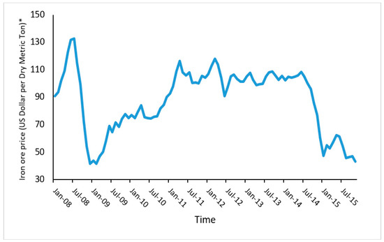
Figure 1.
Monthly variation of iron ore price. * Description: China import Iron Ore Fines 62% FE spot (CFR Tianjin port).
At the moment, pricing of iron ore is based on seasonal agreements of major producers of iron ore and major consumers of steel so that the two markets of Europe and Eastern Asia (in past, Japan and Now, China) have significant role in internal iron ore deals. A major share of distributed iron ore is produced by the three companies of Vale (a semi-private company) (Rio de Janeiro, Brazil ), Rio Tinto(London, UK), and B.H.P Billiton(Melbourne, Australia). Because of the fact that each ton of crude steel is made by using 1.5 ton of iron ore, production of crude steel can be introduced as a demand agent and because provision of iron ore is almost exclusive, producers provide the market with an output totally in association with instant demand [10].
Artificial intelligence, soft computing (SC), and machine learning (ML) techniques such as artificial neural network (ANN) and fuzzy inference system (FIS) have been developed as non-linear tools for solving problems in science and engineering specially in civil and mining fields [11,12,13,14,15,16,17,18,19,20,21,22,23,24,25,26,27,28,29,30,31,32,33,34,35,36,37,38,39,40,41,42,43,44,45,46,47,48]. The use of these techniques in different applications of civil and mining engineering e.g., water and environmental resources [49,50], geotechnical fields [51,52,53,54,55,56], structural and material [13,57,58,59,60], blasting environmental issues [61,62,63,64,65], mineral processing and pricing [7,11,66], transportation planning and design [67,68]. In fact, further engineers and researchers are able to utilize these techniques to get a high level of accuracy for engineering problems.
In the present paper, a new model in the field of mineral price prediction namely group method of data handling (GMDH) is introduced. Literature shows that the models that work on the basis of self-organizing networks containing active neurons (GMDH) are of a higher effectiveness in terms of making more accurate and less labor-intensive predictions. In addition, the paper evaluates the precision of other predictive techniques i.e., autoregressive integrated moving average (ARIMA), ANN, support vector regression (SVR), and classification and regression tree (CART) in predicting monthly price of iron ore. Then, after evaluations of performance predictions of the said models, the best one among them is selected and introduced to solve the problem. In the following parts, after introducing input and output parameters, the principles of predictive models and their implementations in predicting price of iron ore is given in detail. Afterward, the proposed models are evaluated through the use of well-known performance indices and four performance indices are calculated and compared to each other in order to choose the best predictive model.
2. Literature Review
Up to now, different techniques such as statistical and artificial intelligence methods have been suggested for prediction of iron ore price [7]. Traditional mathematical models such as time series [11,69] and the multi linear regression [70,71] models have been used for metals price prediction. One of the most common traditional mathematical models for predicting time series is the autoregressive integrated moving average (ARIMA) method. This technique is one of the most routinely used statistical approaches for time series predicting over the past decades. ARIMA have relished beneficial applications in forecasting insurance, economics, energy, engineering, social, stock problems, and foreign exchange [72,73,74,75]. Critical literature review show that the accuracy of SC and ML techniques is superior to the ARIMA models in predicting time series problems [76,77,78,79,80].
As stated before, the applications of ML and SC techniques have been widely used in fields of civil and mining engineering. In terms of metal and material price prediction, several researchers highlighted a successful implementation of such techniques. For example, Parisi et al. [11] used and developed an ANN model for the prediction of variation of gold prices. They considered the role of ward network in the architecture of the proposed ANN and reported a high ability of the ANN model in forecasting gold price. The monthly copper price was predicted by García and Kristjanpoller [81] proposing ANN and FIS predictive models. They constructed many soft computing models of ANN and FIS and finally concluded that FIS is a more powerful technique in predicting copper price compared to ANN model. In another study, Alameer et al. [82] forecasted a long-term monthly gold price fluctuations by using four ANN-based models i.e., particle swarm optimization (PSO)-ANN, genetic algorithm (GA)-ANN, and whale optimization algorithm (WOA)-ANN and grey wolf optimization-ANN. In fact, they studied the power of these hybrid models in predicting gold price fluctuations and finally, they introduced WOA-ANN as a new and applicable model in this field. Ewees et al. [2] proposed a hybrid intelligent model i.e., chaotic grasshopper optimization algorithm-ANN for estimation of iron ore prices and concluded that their proposed model is a promising technique for forecasting commodity prices with high accuracy. In another study of price prediction, the prediction of coal price fluctuations was considered as the objective by Alameer et al. [83]. They developed three models namely support vector machine (SVM), ANN, and deep neural network (DNN) with the aim to successfully show that the DNN model is able to provide higher performance capacity in estimating coal price fluctuations.
According to the above discussion, the authors decide to use and propose the GMDH which is considered as a new intelligent system in prediction of iron ore price. For comparison purposes, a traditional statistical model, i.e., ARIMA, and three ML techniques i.e., SVR, CART, and ANN are selected to be applied for iron ore price prediction. Then, an evaluation is performed between the applied models and the best model is selected and introduced in field of iron ore price prediction.
3. Input and Output Parameters
In order to estimate the price of iron ore, 12 measurable parameters of highest impact on price of iron ore [84], were defined and considered as input parameters and subsequently, an output parameter was chosen (see Table 1). In Table 1, input and output parameters with their unit, minimum, maximum, and descriptions are presented. All of the existing applied data in the present study was 311 which after using the 10-Fold Cross Validation method, was decreased to 248 number of data from January 1990 to December 2013 (see Figure 2). In the following section, principles and applications of various models i.e., ANN, SVR, GMDH, and CART in predicting price of iron ore are described.

Table 1.
Introducing input and output parameters in the modeling.
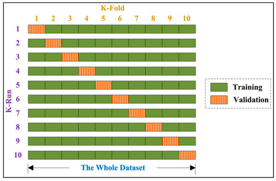
Figure 2.
Ten-fold cross-validation.
4. Applied Methods
4.1. Autoregressive Integrated Moving Average (ARIMA)
Box and Jenkins [85] developed a general forecasting approach to predict future points in the time series. ARIMA can be applied in some cases where data show signal of non-stationarity. In this approach, the future value of a variable is presumed to be a linear function of periodic past explanations and random errors. This model is known as ARIMA (p, q, d), where p stands for number of time lags of the autoregressive model, q is the instruction of moving-average parameters, and d is the number of times the data have had past values subtracted [86]. The 𝑑 parameter is estimated by the number of times the differencing is achieved on the time series [87]. In order to build the best ARIMA model for forecasting of iron ore price, 𝑝 and 𝑞 parameters have to be efficiently determined for a proper model. To estimate the best model, we use the criteria as follows: Bayesian information criterion (BIC), R-squared, root-mean-square error (RMSE), mean absolute percentage error (MAPE), and mean absolute error (MAE). Table 2 shows the different parameters 𝑝, 𝑞, and d in the ARIMA model. ARIMA (0, 1, 1) shows the best performance compared to other presented models in Table 2. The residual plots of autocorrelation function (ACF) and partial autocorrelation function (PACF) in Figure 3 shows the model is adequate as it shows a random variation from the origin zero (0), the points below and above are all uneven, hence the model fitted is acceptable.
Table 2.
Statistical results of different autoregressive integrated moving average (ARIMA) parameters for iron ore price forecasting.
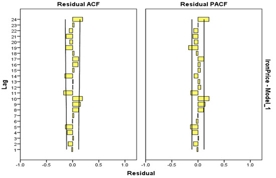
Figure 3.
Residual plots of (ACF) and (PACF) by using ARIMA (0-1-1).
4.2. Classification and Regression Tree (CART)
The decision tree (DT) is one of the non-parametrical approaches for classification purposes. In this approach, a model of classification is introduced for available observation using a very simple technique. The introduced model has a very simple structure, and is comprehensible for decision-making. Although this approach uses simple techniques, it can be performed even sometimes better than complicated approaches such as ANN [88]. The DT has a graph the same as a tree and is composed of roots, branches, leaves, and nodes [65,89]. In this approach, a variable is assigned as root or root node, and each node is then divided into sub-node according to the question about the interval of that variable which is either “Yes” or “No” which in turn indicates an input parameter that includes a prediction of output parameter in itself. Each branch in the DT shows the interval of the node which it is diverged from. The DT is usually drawn from top to bottom so that the roots are located at the top. A leaf is composed of roots, branches, and the final node. The DT includes various algorithms among which CHAID (chi-square automatic interaction detection), QUEST (quick, unbiased and efficient statistical tree), and CART are the most important [90,91]. Reviewing the previous studies indicated that the CART model is more efficient and practical in the field of predicting and simulating compared to the other available ones. Therefore, this algorithm is selected and applied in the present study.
The CART model was developed by Breiman et al. [92] which can be made into a two-scale tree on the basis of some rules. This algorithm gives the capability to be used in parameters concerning quality and quantity. If the dependent parameter is of quantity type, the formed tree is called the “Regression tree,” and if it is of the quality type, it is named “Classification tree.” Parameters such as the “Maximum tree depth” and “Number of intervals” as controlling parameters are taken into consideration in this algorithm to avoid extreme complications of the model [92]. The MATLAB software was used to build the CART model. Many CART models considering the most effective parameters on this model, have been constructed and the best model among them was selected to predict price of iron ore. Figure 4 shows the desirable tree for modelling the iron ore price. In addition, Figure 5 displays the predicted iron ore price by CART verses their measured values. Based on this figure, R2 is determined as 0.936 which revealed that the CART predictive model is able to estimate the iron ore price with high level of accuracy.
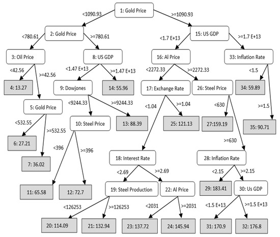
Figure 4.
Regression tress developed for iron ore price.
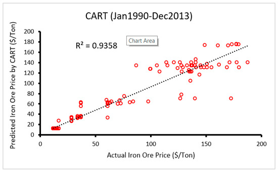
Figure 5.
Scatter plot of the predicted vs. actual iron ore price through the use of classification and regression tree (CART) model.
4.3. Support Vector Regression
Support vector machine (SVM) was introduced to solve both classification and regression problems. Among many methods of machine learning, the SVM is considered as a relatively new technique which is based on the structural risk minimization [93]. SVM can be referred to both regression and classification methods. Among them, support vector regression (SVR) is only able to solve extrapolative problems by building a predictive model. The SVR works based on regression estimation and function approximation considering an alternative “loss function.” The SVR is defined as a common technique which is based on the Vapnik-Chervonenkis (VC) theory [94,95]. If the VC dimension is low, the expected probability of error is also low, which means good generalization [96].
The concept of the ε-insensitive loss function is graphically shown in Figure 6. Only the samples out of the ± ε margin (known as ε-insensitive tube) will have a nonzero slack variable. Normally, if the predicted value is inside the region, the loss will be zero, while if the predicted point is outside the tube, the loss is the magnitude of the difference between the predicted value and the radius ε of the tube.
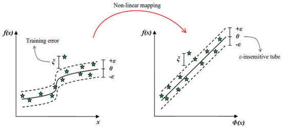
Figure 6.
The concept of the ε-insensitive loss function.
Mentioning about statistical equations behind SVM and SVR is out of scope of this study. In order to have a detailed view of SVM and SVR, studies conducted by Hasanipanah et al. [97] and Mahdevari et al. [98] are suggested. Generally, to construct a SVR model, three factors are very important to determine. These factors are the Gaussian kernel parameter γ, the loss function parameter ε, and the penalty term C [98]. A series models of SVR were built defining a fitness function in three loops for each combination of C, ε, and γ. Then, the optimum C, ε, and γ in each run was selected. Table 3 presents the obtained results of the developed SVR models in terms of performance indices i.e., R2, root mean square error (RMSE) and mean absolute error (Ea). In addition, different combinations of C, ε, and γ can be seen in Table 3. As shown in Table 3, model number 9 (R2 = 0.98, RMSE = 6.63, Ea = 3.84 and) outperforms the others. The results demonstrated a high level of accuracy of SVR in estimating iron ore price. Correlation between predicted and measured values of iron ore price using SVR predictive model is displayed in Figure 7.
Table 3.
Results of ten-fold cross-validation and optimal values of C, ε, and γ in predicting iron ore price.
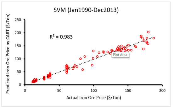
Figure 7.
Scatter plot of the predicted vs. actual iron ore price developing support vector regression (SVR) model.
4.4. Artificial Neural Networks
Artificial neural network (ANN), as it is apparent from their name, are computational networks which are used for simulation of the network of brain neural cells in living creatures. Current knowledge of biologic scientists about the activity of neural neurons in the past few decades is the basis of designing such networks. Neural networks obtain their needed rules through teaching educational teaching. Neural networks use different algorithm for learning but without attention to applied method, learning is generally a repetitive operation during which a set of educational examples are shown to the network so as to help it be thoroughly taught [99,100,101]. So, distribution is the most common learning algorithm of multi-layer neural networks with leading nutrition invented by Rumel Hurt. This method changes connection weights by slope reduction and minimizes error function [61,62,102,103,104,105]. A neural network is composed of a number of neurons in consequent layers. Basically, three layers exist for such networks: an input layer, one or more middle layers in addition to existing neurons in each layer defined based on complexity of the issue through trial-and-error method. A simple network with leading nutrition of input R is presented in Figure 8 [106].
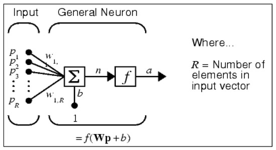
Figure 8.
Structure of a simple neural cell with leading nutrition.
Each input, with suitable weight coefficient (W), is given a weight. Such weights are defined randomly and are corrected during the process of learning with reduction of network error. The sum of weight input and bias make up the input of function of stimulus F. In order to obtain the intended output, one can use a different transfer function. Tangent Sigmoid, logarithm sigmoid, linear and positive linear transfer functions are an example of such functions. In this model, trial-and-error method is used for the two intermediate hidden layers along with addition of logarithm sigmoid transfer function while its output shifts between zero and one. In output layer of leading multi-layer networks, positive linear transfer function was used [107,108,109,110].
Many researchers highlighted application of ANN in various fields of civil and mining works (e.g., [111,112,113]). A number of ANN models with different topology were built and among them, an ANN model with higher accuracy level was chosen. The most influential factors i.e., hidden layer No., No. of nodes in each hidden layer, and the applied transfer function were considered in modeling process. A network with architecture 12-6-1 with minimum error was found to be optimum. R2 was determined between the predicted and the measured values as 0.977 for the optimum ANN model (see Figure 9) which shows capability of this model in predicting iron ore price.
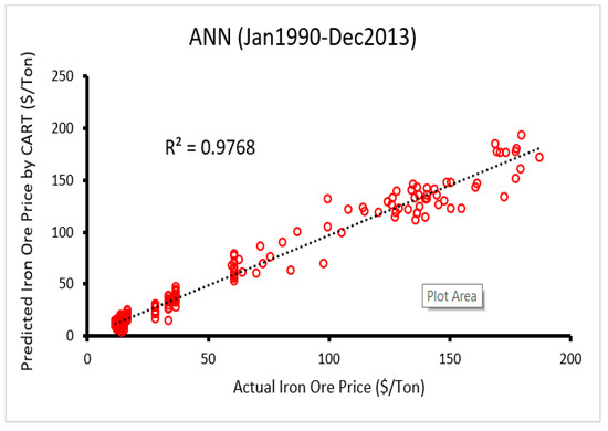
Figure 9.
Scatter plot of the predicted vs. actual iron ore price developing artificial neural network (ANN) model.
4.5. Group Method of Data Handling
GMDH, which was introduced by Ivakhnenko in the 1960s [114], refers to a machine learning technique that works on the basis of the heuristic self-organizing principle [115]. This evolutionary computation technique is able to perform a series of operations like crossbreeding, rearing, seeding, and selection and rejection of seeds corresponding. These operations are related to the determination of the input variables, structure, and parameters of model, and the selection of model by the termination principle [116]. GMDH enjoys a high degree of flexibility and users are able to hybridize it by means of evolutionary and iterative algorithms, e.g., PSO [117], and GA [118]. GMDH helps to represent a model as set of neurons (nodes) wherein various pairs of existing neurons within each layer are linked to each other by quadratic polynomial, thereby generating new neurons in the succeeding layer. This type of representation is applicable to modelling processes for the purpose of mapping inputs to outputs and it can solve almost all non-linear and complex problems. Formally, the system identification problem is described as exploring a function that can be approximately utilized instead of actual function f in a way to estimate the output for a certain input vector X = (x1, x2, x3, …, xn) in a way to be with the minimum distant to its actual output y. Aiming at finding an effective solution, GMDH constructs a general link between the output and input variables which can be in the shape of a mathematical description.
In designing GMDH, all polynomials of the neurons existing within each of the network layers are identical and also the network has been designed on the basis of the same processes. The second-order polynomial is actually the fundamental structure of the GMDH network originally introduced by Ivakhnenko [114]. In general, various types of polynomial, including tri-quadratic, quadratic, bilinear, and third order have been applied to the process of designing the self-organized systems. Compared to the quadratic type of polynomial, with employing the third order and tri-quadratic polynomial, networks of a higher complexity will be constructed. Bilinear polynomial produced lower complicated structure. The quadratic polynomial involves six weighting coefficients that have been found effective in solving engineering problems [119]. Literature shows that selecting one among different types of polynomials depends upon two factors: (1) The minimum error of objective function, and (2) complexity of the polynomial type. In order to get more details about the GMDH model and its implementation, some other studies are suggested [21,114,115].
In order to design a GMDH model, its effective parameters i.e., the number of neurons, the number of GMDH layers, and selection pressure should be taken into consideration. Selection pressure factor is actually a criterion that allows the system to select the best fit in each step and moves them to the next layer. This process is repeated till receiving to the defined criteria which is normally system error. Hence, a parametric study has been conducted to see the effects of this parameter through the trial-and-error procedure. The results showed that selection pressure of 50% can be considered as the one among all values. Therefore, it has been used in the rest of modelling process. The design of another effective parameter (neuron number) on the GMDH model needs another parametric study. To do this, considering the previous studies (e.g., [21]), values of 2, 4, 6, 8, 10, 12, 14, 16, 18, and 20 were selected to be used as number of neurons in the parametric study and results of GMDH models based on R2 are shown in Table 4. Among the obtained results, as it can be seen in Table 4, GMDH model number 8 with 16 neurons shows the best prediction performance and due to that neuron number of 16 was selected in the rest of modelling process. It should be mentioned that this parametric study was conducted using selection pressure of 50% and layer number of 5. In the last step of GMDH modelling, number of layers should be determined through the conduct of another parametric study. For this purpose, amounts of 2, 3, 4, 5, 6, 7, 8, 9, and 10 were set as possible layers number. This was chosen according to previous investigations and their suggestions (e.g., [21]). According to the obtained results of this parametric study (Table 5), R2 of 0.962, 0.968, 0.970, 0.978, 0.976, 0.974, 0.980, 0.977, and 0.978 were achieved for layer numbers of 2, 3, 4, 5, 6, 7, 8, 9, and 10, respectively. The results have clearly confirmed that the layer number 8 (GMDH model number 7) with R2 of 0.980 receives the best performance prediction. Therefore, in design of GMDH model in this study, values of 50%, 16 and 8 were selected for selection pressure, neuron number and layer number, respectively. More discussions about the performance of selected GMDH model will be given in the next section.
Table 4.
The results of parametric study on the number of neurons.
Table 5.
The results of parametric study on the number of layers.
5. Model Evaluation
In this section, evaluation of the developed models for iron ore price prediction is performed. To do this, several performance prediction i.e., R2, RMSE, Ea, MAPE (mean absolute percentage error) and variance account for (VAF) (see Equations (1)–(4)) were chosen and calculated for all developed models i.e., SVR, ANN, CART, and GMDH. Obviously, higher VAF values and lower error values give a model with higher performance prediction.
where, y and y′ are the measured and predicted values, respectively. In addition, N in total number of datasets [120]. In order to validate/test the proposed models, the selected datasets which were not used in the modelling process (23 databases from January 2014 to November 2015) were applied and then predicted. Subsequently, the obtained results from testing step were compared with the measured iron ore price values as shown in Figure 10, Figure 11, Figure 12, Figure 13 and Figure 14 for ARIMA, CART, ANN, SVR, and GMDH models, respectively. As shown in these figures, the measured and predicted values by GMDH are closer to each other compared to other proposed models. This confirmed that the GMDH model which is a new model in the area of this study is able to perform well for prediction of iron ore price. It is a powerful and practical predictive model for such purposes.
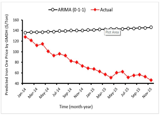
Figure 10.
Comparison between the measured and the predicted by ARIMA model for test stage.
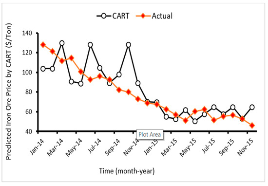
Figure 11.
Comparison between the measured and the predicted by CART model for test stage.
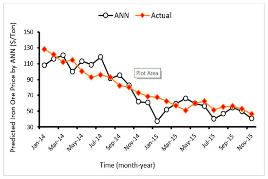
Figure 12.
Comparison between the measured and the predicted by ANN model for test stage.
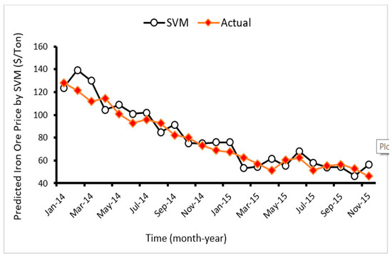
Figure 13.
Comparison between the measured and the predicted by SVR model for test stage.
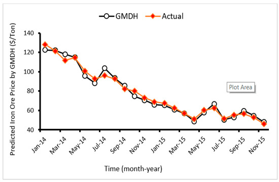
Figure 14.
Comparison between the measured and the predicted by group method of data handling (GMDH) model for test stage.
Aside from that, the obtained results of performance prediction for all proposed techniques are tabulated in Table 6. As it can be seen in this table, higher performance prediction is related to results of GMDH model in both train and test phases. Although the other methods e.g., SVR and ANN are also suitable for prediction purposes and they can provide an acceptable level of accuracy, the highest prediction capacity was achieved developing GMDH predictive approach. Hence, this technique can be introduced as a new predictive model in estimating iron ore price.
Table 6.
The obtained results of performance prediction for testing datasets.
6. Conclusions
The main objective of this study was to propose and introduce a GMDH predictive model as a powerful, capable, and practical one to estimate iron ore price. For comparison purposes, several other techniques i.e., SVR, ANN, ARIMA, and CART were applied and developed to predict iron ore price. For this aim, oil price, steel price, iron ore production, steel production, gold price, inflation rate, exchange rate, interest rate, dowjones stock price, US GDP, aluminum price, China GDP were selected as input variables. A series of analyses with the most effective parameters on the GMDH were conducted in order to see their effects on the system. Then, the best GMDH model was selected among them. Considering several datasets which were not used in the modelling process, the developed models were validated. It was found that the GMDH model which was applied as the first time in the area of this study, could offer more accurate prediction results in comparison with the other implemented models. It was accomplished through the use of some performance prediction such as RMSE and VAF for both model development and model validation. The results of MAPE for testing datasets of GMDH, SVR, ANN, CART, and ARIMA were obtained as 0.039, 0.099, 0.132, 0.169, and 1.001, respectively which show higher prediction capacity of the GMDH technique.
Author Contributions
Formal analysis, M.R.M. and D.J.A.; conceptualization, D.L. and M.M; supervision, M.M. and D.L.; writing—Review and editing, D.J.A. and A.M. All authors have read and agreed to the published version of the manuscript.
Funding
This research was funded by the Outstanding Youth Science Foundations of Hunan Province of China (No. 2019JJ20028).
Conflicts of Interest
The authors declare no conflict of interest.
References
- Pustov, A.; Malanichev, A.; Khobotilov, I. Long-Term iron ore price modeling: Marginal costs vs. incentive price. Resour. Policy 2013, 38, 558–567. [Google Scholar] [CrossRef]
- Ewees, A.A.; Elaziz, M.A.; Alameer, Z.; Ye, H.; Jianhua, Z. Improving multilayer perceptron neural network using chaotic grasshopper optimization algorithm to forecast iron ore price volatility. Resour. Policy 2020, 65, 101555. [Google Scholar] [CrossRef]
- Su, C.-W.; Wang, K.-H.; Chang, H.-L.; Dumitrescu–Peculea, A. Do iron ore price bubbles occur? Resour. Policy 2017, 53, 340–346. [Google Scholar] [CrossRef]
- Nakajima, K.; Daigo, I.; Nansai, K.; Matsubae, K.; Takayanagi, W.; Tomita, M.; Matsuno, Y. Global distribution of material consumption: Nickel, copper, and iron. Resour. Conserv. Recycl. 2018, 133, 369–374. [Google Scholar] [CrossRef]
- Wu, J.; Yang, J.; Ma, L.; Li, Z.; Shen, X. A system analysis of the development strategy of iron ore in China. Resour. Policy 2016, 48, 32–40. [Google Scholar] [CrossRef]
- Sun, S.; Anwar, S. R&D activities and FDI in China’s iron ore mining industry. Econ. Anal. Policy 2019, 62, 47–56. [Google Scholar]
- Ma, W.; Zhu, X.; Wang, M. Forecasting iron ore import and consumption of China using grey model optimized by particle swarm optimization algorithm. Resour. Policy 2013, 38, 613–620. [Google Scholar] [CrossRef]
- Wårell, L. An analysis of iron ore prices during the latest commodity boom. Miner. Econ. 2018, 31, 203–216. [Google Scholar] [CrossRef]
- Lundmark, R.; Nilsson, M. What do economic simulations tell us? Recent mergers in the iron ore industry. Resour. Policy 2003, 29, 111–118. [Google Scholar] [CrossRef]
- Malanichev, A.G.; Vorobyev, P. V Forecast of global steel prices. Stud. Russ. Econ. Dev. 2011, 22, 304. [Google Scholar] [CrossRef]
- Parisi, A.; Parisi, F.; Díaz, D. Forecasting gold price changes: Rolling and recursive neural network models. J. Multinatl. Financ. Manag. 2008, 18, 477–487. [Google Scholar] [CrossRef]
- Lineesh, M.C.; Minu, K.K.; John, C.J. Analysis of nonstationary nonlinear economic time series of gold price: A comparative study. Int. Math. Forum 2010, 5, 1673–1683. [Google Scholar]
- Sarir, P.; Chen, J.; Asteris, P.G.; Armaghani, D.J.; Tahir, M.M. Developing GEP tree-Based, neuro-Swarm, and whale optimization models for evaluation of bearing capacity of concrete-Filled steel tube columns. Eng. Comput. 2019. [Google Scholar] [CrossRef]
- Apostolopoulour, M.; Douvika, M.G.; Kanellopoulos, I.N.; Moropoulou, A.; Asteris, P.G. Prediction of Compressive Strength of Mortars using Artificial Neural Networks. In Proceedings of the Proceedings of the 1st International Conference TMM_CH, Transdisciplinary Multispectral Modelling and Cooperation for the Preservation of Cultural Heritage, Athens, Greece, 10–13 October 2018; pp. 10–13. [Google Scholar]
- Asteris, P.G.; Nikoo, M. Artificial bee colony-Based neural network for the prediction of the fundamental period of infilled frame structures. Neural Comput. Appl. 2019. [Google Scholar] [CrossRef]
- Hajihassani, M.; Abdullah, S.S.; Asteris, P.G.; Armaghani, D.J. A Gene Expression Programming Model for Predicting Tunnel Convergence. Appl. Sci. 2019, 9, 4650. [Google Scholar] [CrossRef]
- Psyllaki, P.; Stamatiou, K.; Iliadis, I.; Mourlas, A.; Asteris, P.; Vaxevanidis, N. Surface treatment of tool steels against galling failure. In Proceedings of the MATEC Web of Conferences, Cape Town, South Africa, 24–26 September 2018; EDP Sciences, 2018; Volume 188, p. 4024. [Google Scholar]
- Xu, H.; Zhou, J.G.; Asteris, P.; Jahed Armaghani, D.; Tahir, M.M. Supervised Machine Learning Techniques to the Prediction of Tunnel Boring Machine Penetration Rate. Appl. Sci. 2019, 9, 3715. [Google Scholar] [CrossRef]
- Harandizadeh, H.; Armaghani, D.J.; Khari, M. A new development of ANFIS–GMDH optimized by PSO to predict pile bearing capacity based on experimental datasets. Eng. Comput. 2019. [Google Scholar] [CrossRef]
- Yang, H.; Koopialipoor, M.; Armaghani, D.J.; Gordan, B.; Khorami, M.; Tahir, M.M. Intelligent design of retaining wall structures under dynamic conditions. STEEL Compos. Struct. 2019, 31, 629–640. [Google Scholar]
- Koopialipoor, M.; Nikouei, S.S.; Marto, A.; Fahimifar, A.; Armaghani, D.J.; Mohamad, E.T. Predicting tunnel boring machine performance through a new model based on the group method of data handling. Bull. Eng. Geol. Environ. 2018, 78, 3799–3813. [Google Scholar] [CrossRef]
- Koopialipoor, M.; Noorbakhsh, A.; Noroozi Ghaleini, E.; Jahed Armaghani, D.; Yagiz, S. A new approach for estimation of rock brittleness based on non-Destructive tests. Nondestruct. Test. Eval. 2019, 34, 1–22. [Google Scholar] [CrossRef]
- Achireko, P.K.; Ansong, G. Stochastic model of mineral prices incorporating neural network and regression analysis. Min. Technol. 2000, 109, 49–54. [Google Scholar] [CrossRef]
- Hasanipanah, M.; Jahed Armaghani, D.; Bakhshandeh Amnieh, H.; Koopialipoor, M.; Arab, H. A Risk-Based Technique to Analyze Flyrock Results Through Rock Engineering System. Geotech. Geol. Eng. 2018, 36, 2247–2260. [Google Scholar] [CrossRef]
- Koopialipoor, M.; Murlidhar, B.R.; Hedayat, A.; Armaghani, D.J.; Gordan, B.; Mohamad, E.T. The use of new intelligent techniques in designing retaining walls. Eng. Comput. 2019. [Google Scholar] [CrossRef]
- Guo, H.; Zhou, J.; Koopialipoor, M.; Armaghani, D.J.; Tahir, M.M. Deep neural network and whale optimization algorithm to assess flyrock induced by blasting. Eng. Comput. 2019. [Google Scholar] [CrossRef]
- Yong, W.; Zhou, J.; Armaghani, D.J.; Tahir, M.M.; Tarinejad, R.; Pham, B.T.; Van Huynh, V. A new hybrid simulated annealing-Based genetic programming technique to predict the ultimate bearing capacity of piles. Eng. Comput. 2020. [Google Scholar] [CrossRef]
- Mahdiyar, A.; Jahed Armaghani, D.; Koopialipoor, M.; Hedayat, A.; Abdullah, A.; Yahya, K. Practical Risk Assessment of Ground Vibrations Resulting from Blasting, Using Gene Expression Programming and Monte Carlo Simulation Techniques. Appl. Sci. 2020, 10, 472. [Google Scholar] [CrossRef]
- Zhou, J.; Guo, H.; Koopialipoor, M.; Armaghani, D.J.; Tahir, M.M. Investigating the effective parameters on the risk levels of rockburst phenomena by developing a hybrid heuristic algorithm. Eng. Comput. 2020. [Google Scholar] [CrossRef]
- Han, H.; Armaghani, D.J.; Tarinejad, R.; Zhou, J.; Tahir, M.M. Random Forest and Bayesian Network Techniques for Probabilistic Prediction of Flyrock Induced by Blasting in Quarry Sites. Nat. Resour. Res. 2020. [Google Scholar] [CrossRef]
- Zhou, J.; Bejarbaneh, B.Y.; Armaghani, D.J.; Tahir, M.M. Forecasting of TBM advance rate in hard rock condition based on artificial neural network and genetic programming techniques. Bull. Eng. Geol. Environ. 2019. [Google Scholar] [CrossRef]
- Zhou, J.; Li, E.; Yang, S.; Wang, M.; Shi, X.; Yao, S.; Mitri, H.S. Slope stability prediction for circular mode failure using gradient boosting machine approach based on an updated database of case histories. Saf. Sci. 2019, 118, 505–518. [Google Scholar] [CrossRef]
- Zhou, J.; Shi, X.; Du, K.; Qiu, X.; Li, X.; Mitri, H.S. Feasibility of random-Forest approach for prediction of ground settlements induced by the construction of a shield-driven tunnel. Int. J. Geomech. 2016, 17, 4016129. [Google Scholar] [CrossRef]
- Asteris, P.G.; Tsaris, A.K.; Cavaleri, L.; Repapis, C.C.; Papalou, A.; Di Trapani, F.; Karypidis, D.F. Prediction of the fundamental period of infilled RC frame structures using artificial neural networks. Comput. Intell. Neurosci. 2016, 2016, 20. [Google Scholar] [CrossRef] [PubMed]
- Zhou, J.; Li, X.; Mitri, H.S. Comparative performance of six supervised learning methods for the development of models of hard rock pillar stability prediction. Nat. Hazards 2015, 79, 291–316. [Google Scholar] [CrossRef]
- Zhou, J.; Li, X.; Mitri, H.S. Evaluation method of rockburst: State-Of-The-Art literature review. Tunn. Undergr. Space Technol. 2018, 81, 632–659. [Google Scholar] [CrossRef]
- Jian, Z.; Shi, X.; Huang, R.; Qiu, X.; Chong, C. Feasibility of stochastic gradient boosting approach for predicting rockburst damage in burst-Prone mines. Trans. Nonferrous Met. Soc. China 2016, 26, 1938–1945. [Google Scholar]
- Zhou, J.; Li, X.; Shi, X. Long-Term prediction model of rockburst in underground openings using heuristic algorithms and support vector machines. Saf. Sci. 2012, 50, 629–644. [Google Scholar] [CrossRef]
- Shi, X.; Jian, Z.; Wu, B.; Huang, D.; Wei, W.E.I. Support vector machines approach to mean particle size of rock fragmentation due to bench blasting prediction. Trans. Nonferrous Met. Soc. China 2012, 22, 432–441. [Google Scholar] [CrossRef]
- Liu, B.; Yang, H.; Karekal, S. Effect of Water Content on Argillization of Mudstone During the Tunnelling process. Rock Mech. Rock Eng. 2019. [Google Scholar] [CrossRef]
- Yang, H.Q.; Li, Z.; Jie, T.Q.; Zhang, Z.Q. Effects of joints on the cutting behavior of disc cutter running on the jointed rock mass. Tunn. Undergr. Space Technol. 2018, 81, 112–120. [Google Scholar] [CrossRef]
- Yang, H.Q.; Zeng, Y.Y.; Lan, Y.F.; Zhou, X.P. Analysis of the excavation damaged zone around a tunnel accounting for geostress and unloading. Int. J. Rock Mech. Min. Sci. 2014, 69, 59–66. [Google Scholar] [CrossRef]
- Chen, H.; Asteris, P.G.; Jahed Armaghani, D.; Gordan, B.; Pham, B.T. Assessing Dynamic Conditions of the Retaining Wall: Developing Two Hybrid Intelligent Models. Appl. Sci. 2019, 9, 1042. [Google Scholar] [CrossRef]
- Asteris, P.G.; Plevris, V. Anisotropic masonry failure criterion using artificial neural networks. Neural Comput. Appl. 2017, 28, 2207–2229. [Google Scholar] [CrossRef]
- Asteris, P.; Roussis, P.; Douvika, M. Feed-Forward neural network prediction of the mechanical properties of sandcrete materials. Sensors 2017, 17, 1344. [Google Scholar] [CrossRef] [PubMed]
- Asteris, P.G.; Ashrafian, A.; Rezaie-Balf, M. Prediction of the compressive strength of self-Compacting concrete using surrogate models. Comput. Concr. 2019, 24, 137–150. [Google Scholar]
- Armaghani, D.J.; Hatzigeorgiou, G.D.; Karamani, C.; Skentou, A.; Zoumpoulaki, I.; Asteris, P.G. Soft computing-Based techniques for concrete beams shear strength. Procedia Struct. Integr. 2019, 17, 924–933. [Google Scholar] [CrossRef]
- Cavaleri, L.; Asteris, P.G.; Psyllaki, P.P.; Douvika, M.G.; Skentou, A.D.; Vaxevanidis, N.M. Prediction of Surface Treatment Effects on the Tribological Performance of Tool Steels Using Artificial Neural Networks. Appl. Sci. 2019, 9, 2788. [Google Scholar] [CrossRef]
- Cheng, C.-T.; Lin, J.-Y.; Sun, Y.-G.; Chau, K. Long-Term prediction of discharges in Manwan Hydropower using adaptive-Network-Based fuzzy inference systems models. In The International Conference on Natural Computation; Springer: Berlin/Heidelberg, Germany, 2005; pp. 1152–1161. [Google Scholar]
- Najafi, B.; Faizollahzadeh Ardabili, S.; Shamshirband, S.; Chau, K.; Rabczuk, T. Application of ANNs, ANFIS and RSM to estimating and optimizing the parameters that affect the yield and cost of biodiesel production. Eng. Appl. Comput. Fluid Mech. 2018, 12, 611–624. [Google Scholar] [CrossRef]
- Alavi Nezhad Khalil Abad, S.V.; Yilmaz, M.; Jahed Armaghani, D.; Tugrul, A. Prediction of the durability of limestone aggregates using computational techniques. Neural Comput. Appl. 2016. [Google Scholar] [CrossRef]
- Armaghani, D.J.; Mohamad, E.T.; Narayanasamy, M.S.; Narita, N.; Yagiz, S. Development of hybrid intelligent models for predicting TBM penetration rate in hard rock condition. Tunn. Undergr. Space Technol. 2017, 63, 29–43. [Google Scholar] [CrossRef]
- Zhou, J.; Li, E.; Wei, H.; Li, C.; Qiao, Q.; Armaghani, D.J. Random Forests and Cubist Algorithms for Predicting Shear Strengths of Rockfill Materials. Appl. Sci. 2019, 9, 1621. [Google Scholar] [CrossRef]
- Armaghani, D.J.; Safari, V.; Fahimifar, A.; Monjezi, M.; Mohammadi, M.A. Uniaxial compressive strength prediction through a new technique based on gene expression programming. Neural Comput. Appl. 2018, 30, 3523–3532. [Google Scholar] [CrossRef]
- Armaghani, D.J.; Koopialipoor, M.; Marto, A.; Yagiz, S. Application of several optimization techniques for estimating TBM advance rate in granitic rocks. J. Rock Mech. Geotech. Eng. 2019. [Google Scholar] [CrossRef]
- Momeni, E.; Nazir, R.; Armaghani, D.J.; Sohaie, H. Bearing capacity of precast thin-Walled foundation in sand. Proc. Inst. Civil Eng. Eng. 2015, 168, 539–550. [Google Scholar] [CrossRef]
- Asteris, P.G.; Apostolopoulou, M.; Skentou, A.D.; Moropoulou, A. Application of artificial neural networks for the prediction of the compressive strength of cement-Based mortars. Comput. Concr. 2019, 24, 329–345. [Google Scholar]
- Chahnasir, E.S.; Zandi, Y.; Shariati, M.; Dehghani, E.; Toghroli, A.; Mohamed, E.T.; Shariati, A.; Safa, M.; Wakil, K.; Khorami, M. Application of support vector machine with firefly algorithm for investigation of the factors affecting the shear strength of angle shear connectors. SMART Struct. Syst. 2018, 22, 413–424. [Google Scholar]
- Toghroli, A.; Suhatril, M.; Ibrahim, Z.; Safa, M.; Shariati, M.; Shamshirband, S. Potential of soft computing approach for evaluating the factors affecting the capacity of steel–Concrete composite beam. J. Intell. Manuf. 2018, 29, 1793–1801. [Google Scholar] [CrossRef]
- Apostolopoulou, M.; Armaghani, D.J.; Bakolas, A.; Douvika, M.G.; Moropoulou, A.; Asteris, P.G. Compressive strength of natural hydraulic lime mortars using soft computing techniques. Procedia Struct. Integr. 2019, 17, 914–923. [Google Scholar] [CrossRef]
- Mohamad, E.T.; Armaghani, D.J.; Noorani, S.A.; Saad, R.; Alvi, S.V.; Abad, N.K. Prediction of flyrock in boulder blasting using artificial neural network. Electron. J. Geotech. Eng. 2012, 17, 2585–2595. [Google Scholar]
- Tonnizam Mohamad, E.; Hajihassani, M.; Jahed Armaghani, D.; Marto, A. Simulation of blasting-Induced air overpressure by means of Artificial Neural Networks. Int. Rev. Model. Simul. 2012, 5, 2501–2506. [Google Scholar]
- Mohamad, E.T.; Armaghani, D.J.; Hajihassani, M.; Faizi, K.; Marto, A. A simulation approach to predict blasting-induced flyrock and size of thrown rocks. Electron. J. Geotech. Eng. 2013, 18, 365–374. [Google Scholar]
- Mohamad, E.T.; Noorani, S.A.; Armaghani, D.J.; Saad, R. Simulation of blasting induced ground vibration by using artificial neural network. Electron. J. Geotech. Eng. 2012, 17, 2571–2584. [Google Scholar]
- Khandelwal, M.; Armaghani, D.J.; Faradonbeh, R.S.; Yellishetty, M.; Majid, M.Z.A.; Monjezi, M. Classification and regression tree technique in estimating peak particle velocity caused by blasting. Eng. Comput. 2017, 33, 45–53. [Google Scholar] [CrossRef]
- Khandelwal, M.; Mahdiyar, A.; Armaghani, D.J.; Singh, T.N.; Fahimifar, A.; Faradonbeh, R.S. An expert system based on hybrid ICA-ANN technique to estimate macerals contents of Indian coals. Environ. Earth Sci. 2017, 76, 399. [Google Scholar] [CrossRef]
- Hoang, N.-D.; Nguyen, Q.-L. A novel method for asphalt pavement crack classification based on image processing and machine learning. Eng. Comput. 2019, 35, 487–498. [Google Scholar] [CrossRef]
- Ellis, K.; Godbole, S.; Marshall, S.; Lanckriet, G.; Staudenmayer, J.; Kerr, J. Identifying active travel behaviors in challenging environments using GPS, accelerometers, and machine learning algorithms. Front. Public Health 2014, 2, 36. [Google Scholar] [CrossRef]
- Shafiee, S.; Topal, E. An overview of global gold market and gold price forecasting. Resour. Policy 2010, 35, 178–189. [Google Scholar] [CrossRef]
- Escribano, A.; Granger, C.W.J. Investigating the relationship between gold and silver prices. J. Forecast. 1998, 17, 81–107. [Google Scholar] [CrossRef]
- Kearney, A.A.; Lombra, R.E. Gold and platinum: Toward solving the price puzzle. Q. Rev. Econ. Financ. 2009, 49, 884–892. [Google Scholar] [CrossRef]
- Jiang, S.; Yang, C.; Guo, J.; Ding, Z. ARIMA forecasting of China’s coal consumption, price and investment by 2030. Energy Sources Part B Econ. Plan. Policy 2018, 13, 190–195. [Google Scholar] [CrossRef]
- Dooley, G.; Lenihan, H. An assessment of time series methods in metal price forecasting. Resour. Policy 2005, 30, 208–217. [Google Scholar] [CrossRef]
- Farhath, Z.A.; Arputhamary, B.; Arockiam, L. A Survey on ARIMA Forecasting Using Time Series Model. Int. J. Comput. Sci. Mob. Comput. 2016, 5, 104–109. [Google Scholar]
- Pai, P.-F.; Lin, C.-S. A hybrid ARIMA and support vector machines model in stock price forecasting. Omega 2005, 33, 497–505. [Google Scholar] [CrossRef]
- Alameer, Z.; Elaziz, M.A.; Ewees, A.A.; Ye, H.; Jianhua, Z. Forecasting copper prices using hybrid adaptive neuro-fuzzy inference system and genetic algorithms. Nat. Resour. Res. 2019, 28, 1385–1401. [Google Scholar] [CrossRef]
- Ahmad, T.; Chen, H. A review on machine learning forecasting growth trends and their real-Time applications in different energy systems. Sustain. Cities Soc. 2019, 102010. [Google Scholar] [CrossRef]
- Matyjaszek, M.; Fernández, P.R.; Krzemień, A.; Wodarski, K.; Valverde, G.F. Forecasting coking coal prices by means of ARIMA models and neural networks, considering the transgenic time series theory. Resour. Policy 2019, 61, 283–292. [Google Scholar] [CrossRef]
- Fischer, J.A.; Pohl, P.; Ratz, D. A machine learning approach to univariate time series forecasting of quarterly earnings. Rev. Quant. Financ. Account. 2020, 1–17. [Google Scholar] [CrossRef]
- Ji, L.; Zou, Y.; He, K.; Zhu, B. Carbon futures price forecasting based with ARIMA-CNN-LSTM model. Procedia Comput. Sci. 2019, 162, 33–38. [Google Scholar] [CrossRef]
- García, D.; Kristjanpoller, W. An adaptive forecasting approach for copper price volatility through hybrid and non-hybrid models. Appl. Soft Comput. 2019, 74, 466–478. [Google Scholar] [CrossRef]
- Alameer, Z.; Elaziz, M.A.; Ewees, A.A.; Ye, H.; Jianhua, Z. Forecasting gold price fluctuations using improved multilayer perceptron neural network and whale optimization algorithm. Resour. Policy 2019, 61, 250–260. [Google Scholar] [CrossRef]
- Alameer, Z.; Fathalla, A.; Li, K.; Ye, H.; Jianhua, Z. Multistep-Ahead forecasting of coal prices using a hybrid deep learning model. Resour. Policy 2020, 65, 101588. [Google Scholar] [CrossRef]
- Zhu, W.; Xu, D. Analysis on the influence factors and fluctuation of iron ore price based on oligopoly market. DEStech Trans. Econ. Bus. Mana. 2016. [Google Scholar] [CrossRef]
- Box, G.E.P.; Jenkins, G.M.; Reinsel, G.C.; Ljung, G.M. Time Series Analysis: Forecasting and Control; John Wiley & Sons: Hoboken, N.J., USA, 2015; ISBN 1118674928. [Google Scholar]
- Contreras, J.; Espinola, R.; Nogales, F.J.; Conejo, A.J. ARIMA models to predict next-day electricity prices. IEEE Trans. Power Syst. 2003, 18, 1014–1020. [Google Scholar] [CrossRef]
- Said, S.E.; Dickey, D.A. Testing for unit roots in autoregressive-moving average models of unknown order. Biometrika 1984, 71, 599–607. [Google Scholar] [CrossRef]
- Kiers, H.A.L.; Rasson, J.P.; Groenen, P.J.F.; Schader, M. Data analysis classification and related methods. In The International Federation of Classification Societies (IFCS); Springer: Namur, Belgium, 2000; p. 428. [Google Scholar]
- Liang, M.; Mohamad, E.T.; Faradonbeh, R.S.; Jahed Armaghani, D.; Ghoraba, S. Rock strength assessment based on regression tree technique. Eng. Comput. 2016, 32, 343–354. [Google Scholar] [CrossRef]
- Stasis, A.C.; Loukis, E.N.; Pavlopoulos, S.A.; Koutsouris, D. Using decision tree algorithms as a basis for a heart sound diagnosis decision support system. In Proceedings of the 4th International IEEE EMBS Special Topic Conference on Information Technology Applications in Biomedicine, Birmingham, UK, 24–26 April 2003; pp. 354–357. [Google Scholar]
- Aher, S.B.; Lobo, L. Comparative study of classification algorithms. Int. J. Inf. Technol. 2012, 5, 239–243. [Google Scholar]
- Breiman, L.; Friedman, J.; Olshen, R.; Stone, C. Classification and regression trees. Wadsworth Int. Group 1984, 37, 237–251. [Google Scholar]
- Gunn, S.R. Support vector machines for classification and regression. ISIS Tech. Rep. 1998, 14, 5–16. [Google Scholar]
- Cortes, C.; Vapnik, V. Support-Vector networks. Mach. Learn. 1995, 20, 273–297. [Google Scholar] [CrossRef]
- Vapnik, V.; Golowich, S.; Smola, A. Support vector method for function approximation, regression estimation, and signal processing. In Advances in Neural Information Processing Systems 9; Mozer, M.C., Jordan, M.I., Petsche, T., Eds.; MIT Press: Cambridge, MA, USA, 1997; pp. 281–287. [Google Scholar]
- Basak, D.; Pal, S.; Patranabis, D.C. Support vector regression. Neural Inf. Process. Rev. 2007, 11, 203–224. [Google Scholar]
- Hasanipanah, M.; Monjezi, M.; Shahnazar, A.; Armaghani, D.J.; Farazmand, A. Feasibility of indirect determination of blast induced ground vibration based on support vector machine. Measurement 2015, 75, 289–297. [Google Scholar] [CrossRef]
- Mahdevari, S.; Shahriar, K.; Yagiz, S.; Shirazi, M.A. A support vector regression model for predicting tunnel boring machine penetration rates. Int. J. Rock Mech. Min. Sci. 2014, 72, 214–229. [Google Scholar] [CrossRef]
- Mohamad, E.T.; Faradonbeh, R.S.; Armaghani, D.J.; Monjezi, M.; Majid, M.Z.A. An optimized ANN model based on genetic algorithm for predicting ripping production. Neural Comput. Appl. 2017, 28, 393–406. [Google Scholar] [CrossRef]
- Mohamad, E.T.; Armaghani, D.J.; Momeni, E.; Yazdavar, A.H.; Ebrahimi, M. Rock strength estimation: A PSO-Based BP approach. Neural Comput. Appl. 2018, 30, 1635–1646. [Google Scholar] [CrossRef]
- Armaghani, D.J.; Mirzaei, F.; Shariati, M.; Trung, N.T.; Shariati, M.; Trnavac, D. Hybrid ANN-Based techniques in predicting cohesion of sandy-Soil combined with fiber. Geomech. Eng. 2020, 20, 191–205. [Google Scholar]
- Khandelwal, M.; Singh, T.N. Prediction of blast-Induced ground vibration using artificial neural network. Int. J. Rock Mech. Min. Sci. 2009, 46, 1214–1222. [Google Scholar] [CrossRef]
- Monjezi, M.; Ghafurikalajahi, M.; Bahrami, A. Prediction of blast-Induced ground vibration using artificial neural networks. Tunn. Undergr. Space Technol. 2011, 26, 46–50. [Google Scholar] [CrossRef]
- Momeni, E.; Nazir, R.; Armaghani, D.J.; Maizir, H. Application of artificial neural network for predicting shaft and tip resistances of concrete piles. Earth Sci. Res. J. 2015, 19, 85–93. [Google Scholar] [CrossRef]
- Khandelwal, M.; Singh, T.N. Evaluation of blast-Induced ground vibration predictors. Soil Dyn. Earthq. Eng. 2007, 27, 116–125. [Google Scholar] [CrossRef]
- Wasserman, P.D. Neural Computing: Theory and Practice; Van Nostrand Reinhold Co.: New York, NY, USA, 1989; ISBN 0442207433. [Google Scholar]
- Monjezi, M.; Bahrami, A.; Varjani, A.Y.; Sayadi, A.R. Prediction and controlling of flyrock in blasting operation using artificial neural network. Arab. J. Geosci. 2011, 4, 421–425. [Google Scholar] [CrossRef]
- Monjezi, M.; Mehrdanesh, A.; Malek, A.; Khandelwal, M. Evaluation of effect of blast design parameters on flyrock using artificial neural networks. Neural Comput. Appl. 2013, 23, 349–356. [Google Scholar] [CrossRef]
- Chen, W.; Sarir, P.; Bui, X.-N.; Nguyen, H.; Tahir, M.M.; Armaghani, D.J. Neuro-Genetic, neuro-Imperialism and genetic programing models in predicting ultimate bearing capacity of pile. Eng. Comput. 2019. [Google Scholar] [CrossRef]
- Gordan, B.; Jahed Armaghani, D.; Hajihassani, M.; Monjezi, M. Prediction of seismic slope stability through combination of particle swarm optimization and neural network. Eng. Comput. 2015, 32, 85–97. [Google Scholar] [CrossRef]
- Khandelwal, M.; Armaghani, D.J. Prediction of Drillability of Rocks with Strength Properties Using a Hybrid GA-ANN Technique. Geotech. Geol. Eng. 2016, 34, 605–620. [Google Scholar] [CrossRef]
- Ghoraba, S.; Monjezi, M.; Talebi, N.; Armaghani, D.J.; Moghaddam, M.R. Estimation of ground vibration produced by blasting operations through intelligent and empirical models. Environ. Earth Sci. 2016, 75. [Google Scholar] [CrossRef]
- Asl, P.F.; Monjezi, M.; Hamidi, J.K.; Armaghani, D.J. Optimization of flyrock and rock fragmentation in the Tajareh limestone mine using metaheuristics method of firefly algorithm. Eng. Comput. 2018, 34. [Google Scholar] [CrossRef]
- Ivakhnenko, A.G. The group method of data of handling; A rival of the method of stochastic approximation. Sov. Autom. Control 1968, 13, 43–55. [Google Scholar]
- Najafzadeh, M.; Barani, G.-A.; Azamathulla, H.M. GMDH to predict scour depth around a pier in cohesive soils. Appl. Ocean Res. 2013, 40, 35–41. [Google Scholar] [CrossRef]
- Ivakhnenko, A.G. Polynomial theory of complex systems. IEEE Trans. Syst. Man. Cybern. 1971, 1, 364–378. [Google Scholar] [CrossRef]
- Onwubolu, G.C. Design of hybrid differential evolution and group method of data handling networks for modeling and prediction. Inf. Sci. (Ny) 2008, 178, 3616–3634. [Google Scholar] [CrossRef]
- Amanifard, N.; Nariman-Zadeh, N.; Farahani, M.H.; Khalkhali, A. Modelling of multiple short-Length-Scale stall cells in an axial compressor using evolved GMDH neural networks. Energy Convers. Manag. 2008, 49, 2588–2594. [Google Scholar] [CrossRef]
- Najafzadeh, M.; Barani, G.-A. Comparison of group method of data handling based genetic programming and back propagation systems to predict scour depth around bridge piers. Sci. Iran. 2011, 18, 1207–1213. [Google Scholar] [CrossRef]
- Mehrdanesh, A.; Monjezi, M.; Sayadi, A.R. Evaluation of effect of rock mass properties on fragmentation using robust techniques. Eng. Comput. 2018, 34, 253–260. [Google Scholar] [CrossRef]


© 2020 by the authors. Licensee MDPI, Basel, Switzerland. This article is an open access article distributed under the terms and conditions of the Creative Commons Attribution (CC BY) license (http://creativecommons.org/licenses/by/4.0/).