Locality-Sensitive Hashing for Information Retrieval System on Multiple GPGPU Devices

Abstract

It is challenging to build a real-time information retrieval system, especially for systems with high-dimensional big data. To structure big data, many hashing algorithms that map similar data items to the same bucket to advance the search have been proposed. Locality-Sensitive Hashing (LSH) is a common approach for reducing the number of dimensions of a data set, by using a family of hash functions and a hash table. The LSH hash table is an additional component that supports the indexing of hash values (keys) for the corresponding data/items. We previously proposed the Dynamic Locality-Sensitive Hashing (DLSH) algorithm with a dynamically structured hash table, optimized for storage in the main memory and General-Purpose computation on Graphics Processing Units (GPGPU) memory. This supports the handling of constantly updated data sets, such as songs, images, or text databases. The DLSH algorithm works effectively with data sets that are updated with high frequency and is compatible with parallel processing. However, the use of a single GPGPU device for processing big data is inadequate, due to the small memory capacity of GPGPU devices. When using multiple GPGPU devices for searching, we need an effective search algorithm to balance the jobs. In this paper, we propose an extension of DLSH for big data sets using multiple GPGPUs, in order to increase the capacity and performance of the information retrieval system. Different search strategies on multiple DLSH clusters are also proposed to adapt our parallelized system. With significant results in terms of performance and accuracy, we show that DLSH can be applied to real-life dynamic database systems.

1. Introduction

With the development of digital content, the typical volume of a database has been growing increasingly larger. Many high-dimensional data sets must be constantly updated, such as audio fingerprint, photo, and text data sets. Managing these data sets requires a suitable dynamic structure [1]. For real-time information retrieval systems, there are two major problems that need to be addressed: First, the search time must be less than a specified time over a large data set. Second, the system is required to return acceptable results (i.e., of high accuracy) for a given query [1,2].

A variety of hashing algorithms have been proposed for high-dimensional data, such as data clustering, dimensionality reduction, hashing, and data classification algorithms, in order to increase the search speed of the Nearest Neighbor Search (NNS) [2,3]. Among these approaches, Locality-Sensitive Hashing (LSH) is an efficient algorithm for data clustering and dimension reduction [3]. According to its principles, LSH divides a data set into multiple buckets with the same similarity factors. Using these similarity factors, we can easily find similar data/items or groups in the data set [4]. Hierarchical LSH can be used by a hierarchical computer system to increase the productivity of a hardware structure or a distributed storage space [5]. We can apply LSH to solve the approximate nearest neighbor problem by calculating the hash value of the query and then find the corresponding bucket by using the family of hash functions. After that, the bucket will indicate the data/items that have high similarity with the input query [4].

The hash table in LSH is a mapping table that indexes the hash value (key) to the list of data/items in the database. Instead of using a dynamic hash table, using a static hash table can increase the search speed [4]. However, when the requirements are changed from a static data set to a dynamic data set, we have to use a different LSH hash table structure to adapt to constantly updated data sets.

In [6], we introduced the Dynamic Locality-Sensitive Hashing (DLSH) algorithm, which can handle constantly updated data sets. However, DLSH uses a more complex hashing structure and that requires more memory usage. The browsing process of DLSH for each bucket requires a large overhead in computational complexity due to it needing to read the additional information. The memory size of a single GPGPU device is limited [7]; thus, it is practically impossible to store the entirety of a big data set on a single GPGPU device. Using multiple GPGPUs is recommended for handling big data with multiple data clusters; each data cluster can be made the necessary size to be stored on a GPGPU device.

When the data set has been separately stored on different GPGPU devices, it is necessary to propose an appropriate search algorithm for multiple sub-data sets of the LSH system, as the system may obtain different results on different sub-data sets.

The main contributions of this paper are increasing the performance of DLSH and reducing the overhead of the search process by using the sequence shuffling approach in a multiple-GPGPU system. The shuffle stage search is mainly introduced to eliminate duplicate search processes on different nodes/cores for the same query array. With its advantages regarding dynamic data sets, it is demonstrated that DLSH is a suitable LSH algorithm for similarity searches in real-world databases.

2. Research Background and Related Works

In this study, we use certain notation to represent the parameters of the system. The most important of these are shown in Table 1.

Table 1. List of abbreviations.

$x,q$	≜	Item, query item
d	≜	Number of dimensions of data
$X=\{x_1,x_2,\dots ,x_n\}$	≜	Data set with n items
$\mathit{s}$	≜	Number of data clusters/slaves
$\widehat{X}=\{X_0,X_1,\dots ,X_{s-1}\}$	≜	Sub-data sets
$H=\{h_1,h_2,\dots ,h_l\}$	≜	Set of l hash functions
$\mathbb{H}$/${\mathbb{H}}_i$	≜	Hash table/Sub-hash tables
$B=\{B_0,B_1,\dots ,B_{\mathit{u}-1}\}$	≜	Set of $u$ buckets in the hash table
$\overrightarrow{x_j}$	≜	Pointer/index to item $x_j$ in X
$\widehat{H}=\{{\widehat{H}}_0,{\widehat{H}}_1,\dots ,{\widehat{H}}_{s-1}\}$	≜	Families of hash functions for clustering
k	≜	Number of kNN results for each query
$Q=\{q_1,q_2,\dots ,q_{\mathit{m}}\}$	≜	Set of $m$ query items
K	≜	Array of kNN results of Q

2.1. k-Nearest Neighbors (kNN) Search Problem

In conventional information retrieval systems, the most crucial problem is finding similar data/items for the input query. Items are considered similar if the distance between them is small, in terms of the associated metric space [8]. Thus, to examine the similarity of two items, we observe the distance between them. There are three common problems related to the similarity searching problem:

Nearest Neighbor Search (NNS) problem: The problem of finding the point $x^{*}\in X$ that is closest to the query point q, using:

$$x^{*}=\mathit{NN}\left(q\right)=\underset{x\in X}{arg\; min}\mathrm{Distance}(q,x),$$

(1)

where $\mathrm{Distance}(,)$ is the distance function in the d-dimensional space ${\mathbb{R}}^d$ and ${arg\; min}_{}\left(\right)$ is the argument of the minimum function, which returns the optimal argument. To find the most similar item to the query, it is necessary to compare the query to all items in the data set [9]. The most similar item can be identified as the nearest neighbor (NN) of the query [8]. However, finding the exact NN is extremely difficult when dealing with a big data set [10].

Approximate Nearest Neighbor (ANN) search problem: the ANN search is a modification of the NNS, which estimates the nearest neighbor using a threshold [10]. Find a point $x\in X$ for the given query point q, in such a way that

$$\mathit{ANN}\left(q\right)=x|\mathrm{Distance}(q,x)\le c\ast \mathrm{Distance}(q,x^{*}),$$

(2)

where $x^{*}$ is the nearest neighbor of q in X and c is the approximation factor.

Using the ANN Search, we can reduce the complexity of the search algorithm by sharply decreasing the number of comparisons between the query point q and points in X [11]. In practice, the distance from the query to its true nearest neighbor is estimated by using a training data set [10]. $P_1$ denotes the estimated threshold for determining the ANN; $P_1$ may be different depending on the requirements of different systems.

Equation (2) becomes:

$$\mathit{ANN}\left(q\right)=x|\mathrm{Distance}(q,x)\le P_1.$$

(3)

k-Nearest Neighbors (kNN) search problem: Using multiple ANN results can increase the convenience of the information retrieval system for real-world cases. We choose k ANN points x for the query q:

$$k\mathit{NN}\left(q\right)=\left\{x\right|\mathrm{Distance}(q,x)\le P_1,x\in X\left\}\mathrm{with}\right|k\mathit{NN}\left(q\right)|=k.$$

(4)

In this study, if the number of accepted items is less than k, we still use k memory locations to store $k\mathit{NN}\left(q\right)$ by setting the empty locations to a NIL value. The item order in $k\mathit{NN}\left(q\right)$ should be sorted by increasing similarity with the query q. Most information retrieval systems using the kNN search provide multiple choices for the user. We consider the kNN search problem as the main problem to solve. To evaluate the performance of kNN search algorithms, accuracy and search time are generally considered as the main metrics [10]. In practice, the system may have multiple candidates; we define the function $CheckANN(q,\overrightarrow{x_j})$ to verify whether the item $x_j$ is one of the kNN results of q or not. The index $\overrightarrow{x_j}$ is used to eliminate memory copying during the search process, in order to increase search performance. Because the kNN results are temporary sorted over time, the qualities of kNN candidates are not only determined by the thresh $P_1$ but also the number of checked items.

2.2. Locality-Sensitive Hashing (LSH)

Note: In this section, we call the data item a point or vector, as we are examining data that include multiple values and dimensions.

LSH uses a family of hash functions to reduce the dimensions of the data set. Then, each hash value in the new, lower-dimensional space forms a bucket containing every data point having that hash value. By using the same hash value, data points in the same bucket are closer than data points in separate buckets. The distances of buckets can also be compared by calculating the distance of hash values in the new metric space. Therefore, LSH is suitable for handling the ANN search problem in cases where the system searches in particular buckets [4,12].

The general LSH algorithm uses a family of hash functions to obtain the hash values. We can choose the suitable hash functions depending on the data type. Random projection functions are frequently used as the hash functions for LSH in the case of processing binary data. We denote the number of subsets or number of hash functions in the family of hash functions as l, $l\le d$. Using l hash functions, LSH generates l subsets for every input point x. This means that there are l random projection functions that transform the d-dimensional space into l-dimensional spaces. The hash table $\mathbb{H}$ of LSH lists all of the hash values and the corresponding data points in the data set. Assuming that we are using a binary hash function, we can obtain a maximum of $2^l$ different hash values, equivalent to $2^l$ buckets [4,12]. Binary hash functions are widely used in the LSH algorithm, as the resulting buckets can easily be identified [12]. We impose the number of buckets u to be equal to $2^l$ in this study.

With a hash table $\mathbb{H}$, we can index all data points to hash values. For the ANN search problem, we must first calculate the hash value v for a query q by using the same set of hash functions H when building $\mathbb{H}$. The hash value v indexes the set of data points $B_v$ in B; these data points will have the same hash value v, where $B=\left\{B_i\right|0\le i<2^l$} is the set of all buckets in $\mathbb{H}$. We can use the NN result on the bucket $B_v$ as the ANN result for the query q:

$${\mathit{ANN}}_{\mathit{LSH}}\left(q\right)=\underset{x\in B_v}{arg\; min}\mathrm{Distance}(q,x).$$

(5)

In practice, a threshold $P_1$ is used to evaluate the accepted distance between the query and its ANN. The function $\mathrm{CheckANN}(q,\overrightarrow{x})$ is used to evaluate the ANN candidates of the query q for all data points $x_i$ in $B_v$. Depending on the limited number of approximate nearest neighbors k, we can stop the comparison when the number of returned neighbors reaches k.

For searching among multiple buckets, LSH needs to search within several buckets $B_{v^{\prime }}$ that have the closest hash values to v. Denote by $P_2$ the threshold for evaluating the similarity between two buckets, where $P_2<P_1$. Then, the distance between the chosen buckets $B_v$ and $B_{v^{\prime }}$ must be less than $P_2$. In this case, we have more opportunities to obtain the approximate nearest neighbor for the query q from other buckets. To find $k{\mathit{NN}}_{\mathit{LSH}}\left(q\right)$ for the query q, LSH conducts search processes on several close buckets to find k nearest neighbors of q in these buckets. The search process for a query in a bucket is called a probe, which is the unit process of the LSH search [4,12].

2.3. StagedLSH

Various modifications have been developed for LSH, in order to increase its performance and/or efficiency. One is StagedLSH, which was proposed in [13] to advance the accuracy of the ANN search in the HiFP2.0 [14] audio fingerprint search system.

Figure 1 demonstrates how to build a hash table with u buckets for a data set X. Each item is divided into 128 sub-frames. After that, the sub-items are collected by grouping three continuous sub-frames, which can be overlapped with each other. As the first and the last sub-frames of an item can only belong to one sub-item, a total of 126 sub-items are created, which can be used to calculate 126 corresponding hash values. After assigning the bucket labels for all items in X, the size of each bucket is obtained. When the memory size for storing the index is determined, we can use u memory units to store the first indices of all buckets. Then, the indices of all items can be stored consecutively following the bucket order on the same inverted file. By using an inverted file, u memory positions are required to index the first items of u buckets. Even if a bucket is empty, StagedLSH needs to use one memory position for it. Each item requires 126∗$\mathrm{sizeof}\left(unit\right)$, in order to store all its hash values. Assuming that one memory position in the inverted file structure requires “$\mathrm{sizeof}\left(unit\right)$” bytes, the size of StagedLSH can be calculated as $(u+n\ast 126)\ast \mathrm{sizeof}\left(unit\right)$ bytes.

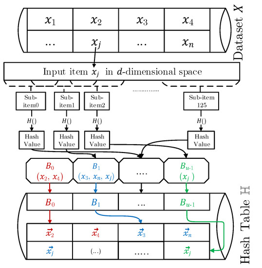
Figure 1. Building the StagedLSH hash table with u buckets and 126 sub-items: Hash all sub-items of all items in the data set X and build an inverted file (Hash table) to index all items by hash values.

In practice, the kNN Result Merger process shown in Figure 2 consists of a serial merger process of the two Temporary Sorted kNN arrays, as shown in Figure 3. As the items in a Temporary Sorted kNN are sorted by their distances to the query q, we can use two iterator variables to look up and fill the best ANN results into another Temporary Sorted kNN. The length of a Temporary Sorted kNN is limited by k, as the system only needs to return k ANN results. The hash table in Figure 2 is stored as an inverted file, which supports its access by parallel threads and takes advantage of data transfer between the CPU and GPGPU. In order to compare the quality of kNN items, we need to use an extra memory unit, to store the similarity with the query beside the index of each item:

$$k{\mathrm{NN}}_{\mathrm{LSH}}\left(q\right)=\{\overrightarrow{x_i},\mathrm{Distance}(q,x_i)|x_i\in X\}\mathrm{with}\left|k{\mathrm{NN}}_{\mathrm{LSH}}\left(q\right)\right|=2k,$$

(6)

the order of items in $k{\mathrm{NN}}_{\mathrm{LSH}}\left(q\right)$ also needs to follow the item order in $k\mathrm{NN}\left(q\right)$, as in Equation (4).

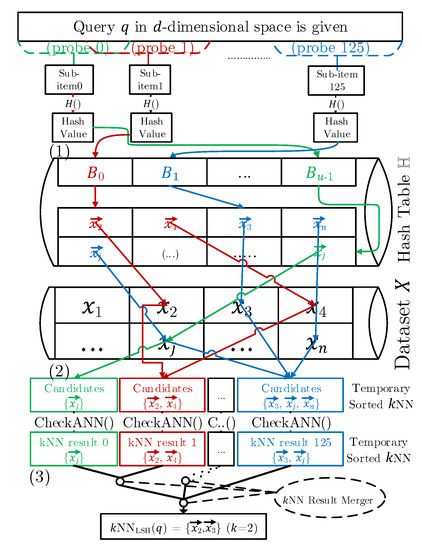
Figure 2. Data flow of StagedLSH search processes of multiple probes: (1) Calculate the hash value for the sub-item; (2) Get list of items in the corresponding bucket; (3) Compare and select the kNN result.

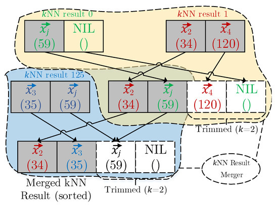
Figure 3. Demonstration of kNN Result Merger for three temporary sorted kNN results, where k = 2.

2.4. kNN Search Using Single GPGPU

In [9], Pan and Jia converted their Bi-Level LSH implementation from CPU to GPU, which uses KD-tree clustering (level 1) for the CPU and LSH search (level 2) for the GPU. They use one CUDA thread to process a single query in the GPU device, which demonstrated that the speed-up ratio could gain up to 40 times, compared to using CPU. In [15], the authors introduced a GPU-based kernelized locality-sensitive hashing method using a single GPU for satellite image retrieval, in which the search process of each query could also be processed by a single GPGPU thread. The methods in [9,15] presented a common bottle-neck problem when multiple queries have different processing times. In that case, the processing time for threads in the same CUDA block can differ greatly, which causes an increase in search time for most queries on the block. Thus, using a single thread for a single query cannot take full advantage of the power of a GPU. In our work, the DLSH algorithm divides the query into multiple small processes (probes), in order to balance the workflow of all CUDA threads. DLSH may have a lower number of concurrent queries; however, it can attain a significant average search speed by increasing the occupancy of the GPGPU.

2.5. kNN Search Using Multiple GPGPUs

Concerning research using multiple GPGPU devices for kNN search, in [16], Kato K. proposed the use of multiple GPU devices for handling multiple kNN search queries simultaneously. Similarly to our study, the method in [16] sends queries to all GPU devices, where each GPU has its own heaps to store temporary ranked kNN candidates and the final kNN results are merged at the end. However, the workflows of the GPU devices in [16] are completely independent of each other; the merging process only takes place when all slaves are done with their searches.

We recognize that this strategy may affect the performance of the whole search system; we called this strategy a “Blind search” in our research, which means that the GPU devices cannot see the current results of others. In [17], Johnson used multiple GPUs to process massive numbers of queries; however, the queries were divided into different GPUs, where each GPU device processed independently. Although there have been several studies using hashing on GPGPU for handing the kNN search problem [17], our study provides a new approach for the optimization of a parallel LSH algorithm using multiple GPGPUs.

In our recommended system, a group of GPGPUs is responsible for parallel searching over all the incoming queries and a Master (CPU) is used to control the workflows of all slaves (i.e., GPGPUs). Computer clusters containing a great number of general-purpose GPUs (GPGPUs) have grown stronger by taking advantage of parallel computing using graphics processing units (GPUs) [18]. The typical locality-sensitive hashing algorithm makes use of different data types and plays different roles in the system. In addition, a raw data set is essential, but its access time is very limited. It is, thus, ideal to store the data set in the GPGPU’s global memory [7]. Furthermore, the memory space required for a family of hash functions is very small, yet its access number is very high due to the calculation of hash values for every query. For this purpose, we can take advantage of the GPGPU’s constant memory, which is small but supports high-speed access.

There exist several public Message Passing Interface (MPI) libraries for the C++ programming language that support use on parallel computers or supercomputers. The target of MPI is to transfer data among processes with high performance and scalability on various systems, as well as portability to different operating systems [19]. By using MPI, a program can be divided into multiple parallel processes; in our system, we use one Master process to control the workflows of the slave processes (GPGPUs). One computer node may have one or multiple GPGPU devices; we deliberately create MPI slave processes to match the number of GPGPU devices on that node. Then, we treat the slave processes fairly, regardless of which node they are in. Each slave process handles GPGPU tasks, such as loading the database, receiving queries, CPU–GPGPU communications, and broadcasting/receiving kNN results.

3. Our Previous Work: Muti-Thread Implementation of StagedLSH on Single GPGPU (CUStagedLSH)

In the first version of DLSH, presented in [6], the DLSH algorithm mainly aims to handle a real, dynamic data set and acquire high-performance parallel processing. This section will discuss the model design, the principles, and multiple-thread optimization of DLSH with a GPGPU.

The traditional search algorithm of StagedLSH uses continuous probes to search multiple buckets with multiple corresponding hash values. For the ANN search problem, StagedLSH can stop in the very first probe when an acceptable item is found. However, StagedLSH has 126 probes for the search process of a query. With the CUStagedLSH search algorithm on a GPGPU, we parallelize the probe processes of the queries in order to increase occupancy.

StagedLSH needs the Merger process to merge the new kNN results after every probe, which involves the duplication of comparisons of the same kNN results after each probe. To avoid this problem, we use multiple CUDA threads to process the StagedLSH probes. As shown in Figure 4, the temporary kNN results are stored in CUDA shared memory and the Merger process can be carried out only one time, after all probes are finished. Using this approach, CUStagedLSH can take advantage of both local memory and shared memory. Thus, CUStagedLSH can handle more kNN results than the original StagedLSH method.

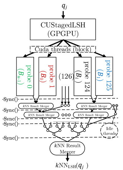
Figure 4. CUStagedLSH: Hardware-oriented optimization of StagedLSH with multiple threads (1 CUDA block) to handle probes related to a query.

Although the original StagedLSH approach uses 126 probes for each query, we deliberately created 128 threads to handle the tasks of 126 probes (where two threads are idle). By allocating 128 ($2^7$) threads, we can optimize the utilization of CUDA’s warp, which has 32 threads in each warp. The shared memory of each block is limited, so we use one block for the process of searching with respect to one query. This helps us to increase the rank size for the candidates of each thread. With 3584 CUDA cores, the P100 device can process 114,688 threads at once. With this number of parallel threads, the P100 GPGPU device is able to process 114,688 probes (i.e., ∼900 queries) in the StagedLSH algorithm in parallel. We realized that a StagedLSH probe is an ideal process for a thread in GPGPU. However, in practical cases, some queries may stop before others, creating an empty slot for the un-processed queries on the same CUDA grid.

A comparison of CUStagedLSH versus other variants of LSH on GPGPU is given in Figure 5. On CPU, CUStagedLSH had a higher search speed than StagedLSH, in cases where these methods had the same recall [6]. However, CUStagedLSH is optimized for processing on GPGPU by parallelizing query probes and using shared memory. This meant that CUStagedLSH could process faster than StagedLSH when using GPGPU. StagedLSH and CUStagedLSH required less hash tables, which meant that StagedLSH and CUStagedLSH could process each probe faster. Entropy-Based LSH [20] has better accuracy when using a selective family of hash functions, but requires a longer amount of time due to the requirements of dynamic hash function allocation. The Basic LSH method was too simple for processing with multiple probes and, so, the recall of Basic LSH was not high, with a single probe for each query.

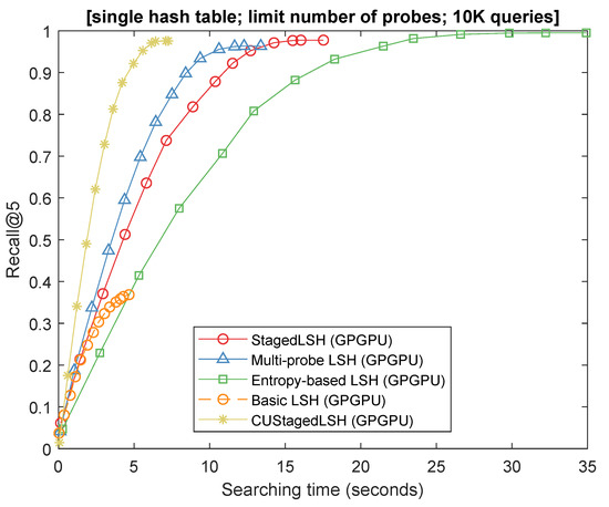
Figure 5. Search time for 10K queries on 1 million audio fingerprints for the approximate kNN search problem using a single GPGPU and the same number of probes.

4. Searching Strategy for Multiple DLSH Clusters on Multiple GPGPU Devices

Figure 6 represents our parallel searching system on multiple GPGPU devices, the data set is clustered using Algorithm 1 and sub-databases are stored by scattering in GPGPU memory. The GPGPU devices have been installed with the CUStagedLSH search method detailed in Section 3. Our model consists of one Master process and several slave processes to control the GPGPU workflows. The Master process accept the queries and broadcasts them to the slaves. After multiple search stages, the Master combines and returns the kNN results of slaves. With this model, we have basically solved the problem of big database management. However, two new problems have arisen in this system, when using multiple devices:

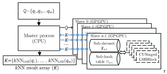
Figure 6. kNN search model with multiple GPGPUs: Master process accepting and forwarding the queries to slaves; Master process receiving and sending kNN result array to s slaves; Master process returning the kNN results array at the end.

• Blind search (Problem 1): The search time for the same query may be different in different slaves. Without communication, the final search time is determined by the slowest slave. For example, slave 0 may need only 1 s to search (best-case scenario), while slave 1 takes 10 s (worst-case scenario); in this case, slave 0 must wait for slave 1 to finish before merging their results.
• Result overflow (Problem 2): The total number of kNN results among multiple slaves may exceed the rank size; that is, the slaves each determine their own kNN results, but the total kNN result may be higher than the rank size. This issue does not affect the accuracy, but the Master process requires more time to select the best kNN results and remove others.

4.1. Multiple StagedLSH Hash Tables

Due to the size of big data, the memory capacity of a single CPU/GPGPU device is not enough: distribution of the database to multiple devices is required. This problem can be tackled using a simple clustering algorithm with proper distance measurement of data/items. It is very important to deploy a clustering algorithm for real-time information retrieval systems.

We recommend using the locality-sensitive hashing clustering algorithm to divide the data into multi-data clusters for distribution. The clustering process will be conducted before generating the hash tables. Figure 7 shows an example of clustering a data set into two sub-databases. The system creates two separate data clusters, which contain different parts of the original data set. Through the use of the LSH hash function family, we can achieve locality-sensitive data/items in the same data cluster, similar to the idea of locality-sensitive data/items in a single bucket.

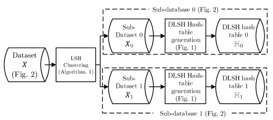
Figure 7. The LSH pre-clustering before generating the StagedLSH hash table of 2 data clusters.

In cases in which the size of the main memory or GPGPU memory is limited, we have to limit the size of each data cluster during the clustering processing. This is a problem for many clustering algorithms, which cannot determine the limiting size for each data cluster.

We propose the use of a different list of the families of hash functions to cluster the data set. In Algorithm 1, ${\widehat{H}}_0$ is the main family of hash functions for clustering, which is used to calculate the hashing index ${\widehat{H}}_i$ of x. The data x will be directly assigned to a data cluster $C_{x,0}$, if possible. Whenever the limiting size of a data cluster $C_{x,0}$ is reached, we use the alternative hash family functions. The testing processes of these alternative ${\widehat{H}}_i$ will check other appropriate probes $C_{x,i}$ to assign the current x. This approach can also resolve the problem in which the number of devices is less than the output range of the hash function, by setting the upper bound sizes of excess data clusters to zero.

Algorithm 1 LSH clustering approach for achieving limited-size data clusters.

Require: Data set X, $\widehat{H}=\{{\widehat{H}}_0,{\widehat{H}}_1,\dots ,{\widehat{H}}_{s-1}\}$ (s hash functions each) Ensure: Clustering the data set X into s data clusters {$X_0,\dots ,X_{s-1}$} with limited size of data clusters  1: {$X_0,\dots ,X_{s-1}$} ← {∅, …}                           ▹ Initialize  2: for eachx in X do  3:   for each family of hash function ${\widehat{H}}_i$ in $\widehat{H}$ do  4:    $hash$ ← ${\widehat{H}}_i$(x)                           ▹ 0 ≤$hash$ < s  5:    if !Is_Full($X_{hash}$) then  6:     $X_{hash}$ ← $X_{hash}\cup x$  7:     Break  8:    end if  9:   end for 10:   if data cluster for x was not assigned then 11:    $X_i\leftarrow$ Random data cluster that is not full. 12:    $X_i$ ← $X_i\cup x$ 13:   end if 14: end for 15: return {$X_0,\dots ,X_{s-1}$}

4.2. Multi-Stage Search

To overcome Problem 1 (Blind search), we propose to divide the search processing for queries into small stages. We create memory space for the Master and slave’s kNN results before the search process starts. After each stage, these memory spaces are synchronized among the MPI processes. The new kNN results are added to the empty slots after synchronization. Therefore, the Multi-stage search of a query can be stopped when the kNN result memory is filled. This helps to eliminate Problem 1. An example is shown in Figure 8, where the search processes of $q_5$ and $q_6$ can be stopped after stages 0 and 1, respectively. The kNN result array K is the collection of kNN results for every query q in Q:

$$K=\{k{\mathrm{NN}}_{\mathrm{LSH}}\left(q_1\right),\dots ,k{\mathrm{NN}}_{\mathrm{LSH}}\left(q_m\right)\}.$$

(7)

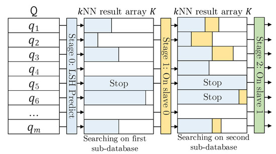
Figure 8. Multi-stage search for an array of queries with multiple slaves.

However, there is still the problem of the worst-case scenario happening in an early stage, which causes the search time to be non-optimal (Query 3 in Figure 8 is an example). We can greatly reduce this problem by using a heuristic data cluster-selection scheme, which tries to search for the kNN results of a query in the slaves with a high likelihood of obtaining good kNN results first. The first search stage in the multi-stage search always takes part in the data cluster that has the same hash value as the query. In this case, we reuse the family of hash function ${\widehat{H}}_0$ for data clustering to calculate this Level 1 LSH. After the first search state, the query uses probes in the nearest data clusters to the data cluster that was searched first.

4.3. Shuffling Parallel LSH Search (S-PLSH) for Multiple DLSH Clusters

S-PLSH is a Multi-stage search strategy that attempts to address Problem 2. S-PLSH can guarantee that the search probe of a query is only conducted by one slave at a time. This helps to reduce the result overflow of all queries in the buffer. By using S-PLSH, the searching order of slaves may be changed.

The shuffling search method includes multiple stages and requires transferring the results from a slave to other slaves. In Figure 9, the CUStagedLSH clusters have two devices/slaves and, so, there is a maximum of (2 + 1) shuffle stages for the list of queries.

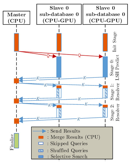
Figure 9. Parallel shuffling search of multiple StagedLSH data clusters with MPI for 2 devices.

Algorithm 2 shows the scheduling of multiple slaves in the system. First, the Master transfers the query array to all slaves. The first search stage is the most important search stage, which uses the LSH hash function to predict the buckets of all queries within it. Then, after Stage 0, two slaves need to update their results to the Master, following which the Master updates its kNN results with the new ones before sending them back to the slaves. Note that there are several queries among the slaves that cannot find their ANNs due to a missed device. Before starting the resolver stages, each slave only needs to process $\mathrm{shuffle}\_\mathrm{size}=m/s$ of the unsolved queries, where m is the size of the query buffer and s is the number of slaves.

Obviously, a higher number of slaves/devices leads to a higher number of search stages in S-PLSH. For a slave, a search stage of S-PLSH searches an average of $m/s$ queries, and there is a maximum of $s+1$ search stages (one LSH Prediction stage and s Resolver stages). However, the number of kNN results received decreases, due to sufficient content or data cluster misses; therefore, we suggest cutting out a number of final search stages, in order to increase the search speed for the trade-off of decreased kNN result quality. After conducting experiments, we suggest the use of 2–4 Resolver stages, in order to balance the speed and accuracy of S-PLSH.

Another issue related to S-PLSH’s scalability is the overhead of the MPI message when using a high number of slaves. If m is the number of queries and k is the number of kNN results, an ANN result uses $2\ast \mathrm{sizeof}\left(unit\right)$ bytes of storage (one unit for the index and one for the distance), and an MPI message for synchronization requires $2km\ast \mathrm{sizeof}\left(unit\right)$ bytes as the content size. With s slaves, we have total of $2s$ messages to be sent. However, from the second search stage, the messages only contain $2k/s$ results to be sent to the Master and, so, the total size required for S-PLSH is $2kms(2+s)\ast \mathrm{sizeof}\left(unit\right)$ bytes for the whole search process. It is clear that the total content size of the packages varies linearly with the number of slaves and queries. This indicates that this topology is superior to that of broadcasting MPI messages from slaves to slaves, which requires $s^2-s$ MPI messages in each synchronization step.

Algorithm 2 S-PLSH search pseudocode on CUStagedLSH slave.

Require:$Q=\{q_1,q_2,\dots ,q_m\}$, slave_ID, corresponding sub-database Ensure: RESULT (kNN result array)  1: Initialize the system: Each slave loads its data set and hash table into main memory and GPGPU memory  2: Transfer Query buffer: Master node transfers the query buffer Q to all slave; Allocate RESULT for all processes  3: State 0:                               ▹LSH Prediction stage  4: for query q in Q do  5:   if H(q) == slave_ID then  6:    RESULT[q] ← CUStagedLSHSearch(q)  7:   end if  8: end for  9: Synchronize RESULT array with the Master and other slaves. 10: Resolver State i (0 ≤ i < m):                       ▹ Resolver stages 11: shuffle_size ← $m/s$ 12: shuffle_index ← shuffle_size*((slave_ID+i) $mod$m) 13: $Q^{\prime }$ ← Q(shuffle_index:shuffle_size) 14: for query q in $Q^{\prime }$ do 15:   if Not_Full(RESULT[q]) then 16:    RESULT[q] ← RESULT[q] ∩ CUStagedLSHSearch(q) 17:   end if 18: end for 19: Synchronize kNN result array with the Master. 20: return

5. Experimental Setup

Our target is to demonstrate that the proposed dynamic information retrieval system can work effectively on the Collaborative Filtering (CF) problem and, in particular, the kNN search problem. As real-time querying of the similarity content of audio/images is a common problem at present, we tested our system with a data set comprised of millions of audio fingerprints.

We aim to examine the impact of our proposed system on a large memory space with an enormous amount of data in the database. With the typical size of a HiFP2.0 feature being 512 bytes, for the test, we generated a set of 64 million HiFP2.0 features with a total size of 62 GB. To analyze the accuracy of both LSH and CUStagedLSH systems, we created numerous testing queries with different distortions from the data set and examined different numbers of hash functions in the generated family of hash functions.

The query set contained 10,000 items that differ from items in the data set, where every query item had its own ground truth kNN set containing the indices of items in the data set (32 true NNs for each query). The accuracy of kNN was examined by the percentage of correct results compared to the ground truth sets (i.e., the sets of true NNs to the queries in the data set). The recall is an accuracy measurement for a group of queries, which can be calculated as:

$${\mathrm{Recall}}_k\left(Q\right)=\frac{1}{m}\sum _{q\in Q}^{}\frac{|k\mathrm{NN}\left(q\right)\cap \mathrm{GT}k{\mathrm{NN}}_k\left(q\right)|}{k},$$

(8)

where $k\mathrm{NN}\left(q\right)$ is the kNN results of query q after searching and $\mathrm{GT}k{\mathrm{NN}}_k\left(q\right)$ is the ground truth kNN set for q. The precision was not important, as our method used the threshold to check the kNN candidates and ranked them in every probe.

The specifications of the testing computer are shown in Table 2. Each testing node had two P100 GPGPU devices and was able to create 32 MPI parallel processes.

Table 2. Specifications of each testing node (8 nodes total).

CPU	Intel Xeon Gold 6130 32 Cores
CPU Clocks	2.1 GHz
Main Memory	64 GB
Bandwidth (internal node)	3088 MB/s
Bandwidth (between nodes)	1202 MB/s
GPGPU	Tesla P100 (×2)
GPGPU Clocks	1328 MHz
GPGPU Memory	16 GB (×2) (GDDR5)
CUDA version	9.1
Recall reduction (4 nodes vs. 1 node)	0.083%

6. Results and Comparison

6.1. Performance of S-PLSH on Multiple GPGPU Devices

First, we carried out experiments of Multi-stage search and S-PLSH, with different numbers of GPGPU devices.

As shown in Figure 10, when dealing with the same database that has the same number of queries, using multiple data clusters (Blind search) helps to reduce the search time by parallel processing on multiple processes. With a higher number of slaves, we can achieve a lower memory size of the database for each data cluster. The S-PLSH algorithm resulted in a shorter search time than Multi-stage search and Blind search, as used in [16], by skipping numerous probes. However, S-PLSH took time to share information among data clusters. As shown in Figure 11, the recall of S-PLSH was comparable with recall of Multi-stage search and Blind search. As S-PLSH has the potential to skip the probes that have true approximate neighbors with the same similarity as the candidates on other data clusters, the accuracy of S-PLSH slightly decreased when the number of slaves increased.

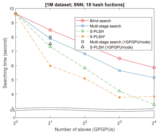
Figure 10. Search time in basic parallel searches and S-PLSH searches on multiple CPUs and GPUs with 10K queries on 1 million audio fingerprints.

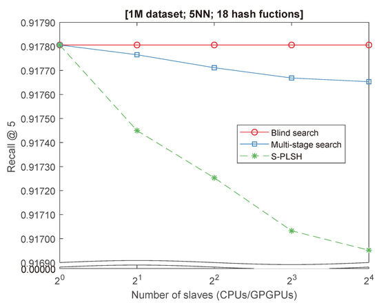
Figure 11. Recall of basic parallel searches and S-PLSH searches on multiple CPUs and GPUs with 10K queries on 1 million audio fingerprints.

In addition, in the case of the system with multiple slaves, the search speed can be affected by the bandwidth. Figure 10 shows the differences in slave search times on the same and different nodes. This shows, in the case of two slaves, the overhead of searching on different nodes (1 GPGPU/node) was about 5–7%. In addition, the distance computation between items takes most of the time in the searching process. When using HiFP2.0 audio fingerprint, taking bit-to-bit XOR operations for the sequences of 4096 bits takes more GPGPU clock cycles than the hashing computation of the vector of 4096 bits.

The impact of different synchronization strategies is shown in Figure 10, where S-PLSH* is the S-PLSH search using MPI messages broadcasted among slaves without using the Master as an intermediary. With a small number of slaves (e.g., 2–8), S-PLSH* showed better performance than S-PLSH, due to the fast transfer. It is clear that, with 10,000 HiFP2.0 features on 16 slaves, S-PLSH sent a total of 2.5 MB/(32 messages) of data for synchronization while S-PLSH* needed 18.75 MB/(240 messages). These amounts of memory were small, compared to the network bandwidth in the test computer. This indicates that the results are acceptable. There was a trade-off between bandwidth and performance in S-PLSH’s strategies. For this reason, S-PLSH* is not recommended for use in a search system with a higher number of slaves or with small bandwidth.

The synchronization performance results are shown in Figure 12. The linear effect of the number of items is clearly shown in this chart. As the message size is smaller with a higher number of slaves, our system was able to process more queries. To send large messages, we could divide them into small messages and send them multiple times. However, the sending time will sharply increase, due to the overhead of sending and receiving packages and management cost. The networks between processes on the same node were always faster than networks on different nodes, which made the synchronization time of eight slaves on two nodes higher than that of eight slaves on the same node. With 16 slaves, we could process the result synchronization process of 1 million queries in 5 s. However, in real-world cases, we do not need to process that many queries at once. Instead, we can split them up to ensure the maximum search time for all queries. The network in supercomputer become faster and faster, that makes our proposed system can reduce the overhead for sending and receiving data.

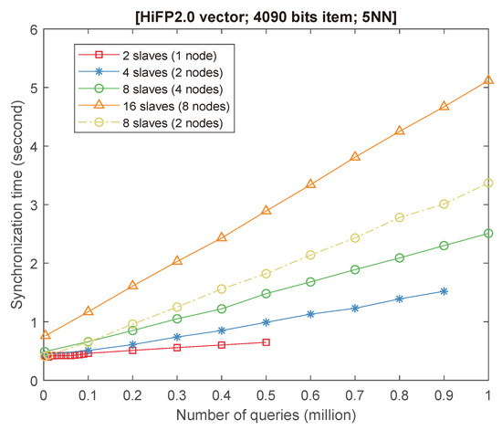
Figure 12. Synchronization time for different number of slaves vs. buffer size.

Finally, Figure 13 shows the scalability of S-PLSH for the big data set. We used most of the storage capacity of one P100 GPGPU (which had 16 GB memory) to store the database of 16 million HiFP2.0 audio fingerprints. Therefore, by using eight P100 GPGPUs, we could store the database of 64 million HiFP2.0 audio fingerprints. With the GPGPU, it was obvious that the search time of the system of eight slaves on 64 million items was similar to that of the system of four slaves on 32 million items, as the kernel of each slave had the same amount of tasks. However, the search processes in a CPU are serial, and the system can stop the search process of an earlier query before changing to other queries. This makes the searching process of a system using a CPU along with a with higher number of GPGPU shorter.

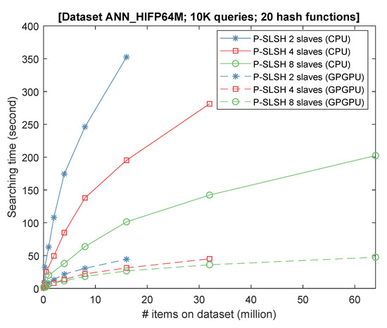
Figure 13. Search time of S-PLSH on the big data set with multiple GPGPUs.

6.2. Comparisons

Table 3 compares the differences of our proposed system with other recent LSH distributed systems. PLSH [21] can support a dynamic data set by using a buffer for storing the new data/items that need to be added to the database. However, the PLSH system requires an interval updating process to add this buffer into the stable database. During that time, the temporary data/items cannot be reached for the NNS problem. Our method employs a single LSH data cluster per each node/device, which is more compatible with GPGPU memory. Further, SES-LSH [22] stores multiple LSH data clusters to increase performance by searching only in selected data clusters. This approach means that our method achieved more accuracy by fully shuffling the queries into all data clusters. We used more network connections among nodes and GPUDirect to reduce the computation of the Master node. This resulted in a reduction in the performance of our system, but meant our system had the best accuracy compared to other similar systems.

Table 3. The advantages and disadvantages of S-PLSH versus other recent multiple LSH cluster systems.

	S-PLSH	SES-LSH	PLSH
Dynamic Data set	Yes	No	Buffered
Data clusters/Node	1	Multiple	1
Network connections	2n	2(n-1)	N/A
GPGPU Support	Yes	No	No
Fully shuffle search	Yes	No	N/A
Distributed HashTable	Yes	Yes	Yes
Hierarchical Searching	Yes	No	Yes
Parallel Searching	Yes	Yes	No
Speed	High	Normal	High

7. Conclusions

The proposed search method in this paper can work efficiently for both CPUs and GPGPUs. However, the use of GPGPUs is entirely suitable for an online real-time information retrieval system. As the memory size of a single GPGPU device is limited, we recommend clustering the data for multiple GPGPU devices. We also proposed a parallel shuffling search for multiple parallel data clusters. The S-PLSH method reduces the duplicated searching process by sharing information among nodes and sequentially swapping parts of the search array. S-PLSH can be reconfigured to suit different data sets and computer systems.

With the advantages of S-PLSH, the information retrieval systems using big data such as identify content that infringes copyright for audio, video, text or images can archive higher performance with the acceleration of GPGPU. On the other hand, the CUStagedLSH helps to handle numerous queries at once by increasing the occupancy of GPGPUs.

For future work, we will focus on optimizing the parallel shuffling search. We aim to reduce the network traffic between slaves, in order to increase the performance of parallel CUStagedLSH on computers with a massive number of nodes.

References

- Bello-Orgaz, G.; Jung, J.J.; Camacho, D. Social big data: Recent achievements and new challenges. Inf. Fusion 2016, 28, 45–59. [Google Scholar] [CrossRef]
- Chen, M.; Mao, S.; Liu, Y. Big data: A survey. Mob. Netw. Appl. 2014, 19, 171–209. [Google Scholar] [CrossRef]
- Park, J.S.; Chen, M.S.; Yu, P.S. An Effective Hash-Based Algorithm for Mining Association Rules; ACM: New York, NY, USA, 1995; Volume 24. [Google Scholar]
- Datar, M.; Immorlica, N.; Indyk, P.; Mirrokni, V.S. Locality-sensitive hashing scheme based on p-stable distributions. In Proceedings of the Twentieth Annual Symposium On Computational Geometry, Brooklyn, NY, USA, 9–11 June 2014; ACM: New York, NY, USA, 2004; pp. 253–262. [Google Scholar]
- Blanas, S.; Li, Y.; Patel, J.M. Design and evaluation of main memory hash join algorithms for multi-core CPUs. In Proceedings of the 2011 ACM SIGMOD International Conference on Management of Data, Athens, Greece, 12–16 June 2011; ACM: New York, NY, USA, 2011; pp. 37–48. [Google Scholar]
- Mau, T.N.; Inoguchi, Y. Scalable Dynamic Locality-Sensitive Hashing for Structured Dataset on Main Memory and GPGPU Memory. Available online: https://airccj.org/CSCP/vol8/csit89715.pdf (accessed on 2 March 2020).
- CUDA Nvidia. Nvidia Cuda C Programming Guide. Available online: https://docs.nvidia.com/cuda/cuda-c-programming-guide/index.html (accessed on 2 March 2020).
- Desrosiers, C.; Karypis, G. A comprehensive survey of neighborhood-based recommendation methods. In Recommender Systems Handbook; Springer: Boston, MA, USA, 2011; pp. 107–144. [Google Scholar]
- Pan, J.; Manocha, D. Fast GPU-based locality sensitive hashing for k-nearest neighbor computation. In Proceedings of the 19th ACM SIGSPATIAL International Conference on Advances in Geographic Information Systems, Chicago, IL, USA, 1–4 November 2011; ACM: New York, NY, USA, 2011; pp. 211–220. [Google Scholar]
- Chang, E.Y. Approximate High-Dimensional Indexing with Kernel. In Foundations of Large-Scale Multimedia Information Management and Retrieval; Springer: Berlin/Heidelberg, Germany, 2011; pp. 231–258. [Google Scholar]
- Andoni, A.; Indyk, P. Near-optimal hashing algorithms for approximate nearest neighbor in high dimensions. In Proceedings of the FOCS’06, 47th Annual IEEE Symposium on Foundations of Computer Science, Berkeley, CA, USA, 21–24 October 2006; pp. 459–468. [Google Scholar]
- Cen, W.; Miao, K. An improved algorithm for locality-sensitive hashing. In Proceedings of the 2015 10th International Conference on Computer Science & Education (ICCSE), Cambridge, UK, 22–24 July 2015; pp. 61–64. [Google Scholar]
- Yang, F.; Sato, Y.; Tan, Y.; Inoguchi, Y. Searching acceleration for audio fingerprinting system. In Proceedings of the Joint Conference of Hokuriku Chapters of Electrical Societies, Imizu, Japan, 1–2 September 2012; Available online: https://www.ieice.org/hokuriku/h24/jhes.htm (accessed on 2 March 2020).
- Araki, K.; Sato, Y.; Jain, V.K.; Inoguchi, Y. Performance evaluation of audio fingerprint generation using haar wavelet transform. In Proceedings of the International Workshop on Nonlinear Circuits, Communications and Signal Processing, Tianjin, China, 1–3 March 2011; pp. 380–383. [Google Scholar]
- Lukač, N.; Žalik, B.; Cui, S.; Datcu, M. GPU-based kernelized locality-sensitive hashing for satellite image retrieval. In Proceedings of the 2015 IEEE International Geoscience and Remote Sensing Symposium (IGARSS), Milan, Italy, 26–31 July 2015; pp. 1468–1471. [Google Scholar]
- Kato, K.; Hosino, T. Multi-GPU algorithm for k-nearest neighbor problem. Concurr. Comput. Pract. Exp. 2012, 24, 45–53. [Google Scholar] [CrossRef]
- Johnson, J.; Douze, M.; Jégou, H. Billion-scale similarity search with GPUs. IEEE Trans. Big Data 2019. [Google Scholar] [CrossRef]
- An Acceleration Superhighway To the AI Era. IBM Power System AC922. 2018. Available online: https://www.ibm.com/us-en/marketplace/power-systems-ac922/details (accessed on 2 March 2020).
- Barker, B. Message passing interface (mpi). In Workshop: High Performance Computing on Stampede; Cornell University Publisher: Houston, TX, USA, 2015; Volume 262, Available online: https://www.cac.cornell.edu/education/training/StampedeJan2015.aspx (accessed on 2 March 2020).
- Wang, Q.; Guo, Z.; Liu, G.; Guo, J. Entropy based locality sensitive hashing. In Proceedings of the 2012 IEEE International Conference on Acoustics, Speech and Signal Processing (ICASSP), Kyoto, Japan, 25–30 March 2012; pp. 1045–1048. [Google Scholar]
- Sundaram, N.; Turmukhametova, A.; NSatish, N.; Mostak, T.; Indyk, P.; Madden, S.; Dubey, P. Streaming similarity search over one billion tweets using parallel locality-sensitive hashing. Proc. VLDB Endow. 2013, 6, 1930–1941. [Google Scholar] [CrossRef]
- Li, D.; Zhang, W.; Shen, S.; Zhang, Y. SES-LSH: Shuffle-Efficient Locality Sensitive Hashing for Distributed Similarity Search. In Proceedings of the 2017 IEEE International Conference on Web Services (ICWS), Honolulu, HI, USA, 25–30 June 2017; pp. 822–827. [Google Scholar]
© 2020 by the authors. Licensee MDPI, Basel, Switzerland. This article is an open access article distributed under the terms and conditions of the Creative Commons Attribution (CC BY) license (http://creativecommons.org/licenses/by/4.0/).