Abstract
Herein, the authors publish the complex design of a numerical coupled model of a vibration-based harvester that transforms mechanical vibrations into electric energy. A numerical model is based on usage of the finite element method, connecting analysis of the damped mechanical oscillation, electromagnetic field and electrical circuit. The model was demonstrated on the design of a microgenerator (MG), and then experimentally tested. The numerical model allows us to execute optimization of the design with many degrees of freedom. The transformation of the wave spreading in the form of mechanical vibrations was solved in the area of resonance of the electromechanical system.
1. Introduction
The extraction of residual energy (harvesting) has been a subject of scientific research in the latest decade. In many projects and publications [1,2,3,4,5,6,7,8,9,10,11,12,13,14,15,16,17,18,19], the arrangement of a system generating electric power is sought as a suitable or optimized solution of design proposals. A very satisfactory tool of basic research is numerical modeling [2,3,4,8,17,18,19]. It can be very robust [2], but also can only be used as a tool for partially solving the hybrid modeling approach [8].
One of the prerequisites for the design of the electromechanical system is a correct way of grasping the physical principle for maximum description of phenomena and processes; it is fundamental in harvesting extraction, as cases in the theses and works [17,18,19]. When comparing the majority of experimental methods and approaches [9,20], including hybrid design methods [6,7,8] with numerically modeled coupled tasks, the realized design using finite element methods (FEM) [2] is difficult to process but it leads to results with significant parameters relative to other quick approaches, as reported in work [19], Table 1, column “Effective power density [W/m3]”.
In Figure 1, an example is shown of a principal design of a harvester model based on the principle of electromagnetic induction using the Faraday induction law in its full range [2,19]. The analysis and results evaluation were based on the numerical model solved by the FEM.
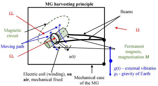
Figure 1.
The principal configuration of the core of the minigenerator a beam version (BV).
The critical parameter can be, for example, the boundary sensitivity of the generator to the minimum vibration amplitude. For the studied design the acceleration value is G = 0.01 g − 0.05 g (g = 9.81 m/s−2). Minimal external dimensions of the microgenerator (MG) had to be found and simultaneously, the expected volume was in the range of VMG = (10 − 50) × 0.10−6 m3. Further, the range of expected output effective power (RMS) was Pout =10–100mW, expected output voltage range Uout =2–20V and excitation frequency range fs =15–35 Hz. The principle of resonant arrangement of the moving MG core was used to attain a high efficiency of the vibration transformation, Figure 1. For moving path selection as linear part with non-linear magnetic braking system (Figure 2a), this concept was fully numerically modeled using the associated FEM model (112) described below. It has been shown that the technical solution of the MG core conductor designed within our approach leads to an increase in the damping coefficient and it does not have sufficient sensitivity to lowest acceleration values in the range G = 0.01 g − 0.02 g. Therefore, the concept of beam version (BV) in the arrangement, Figure 2b,c was approached in the solution. Thus the designed and tested MG achieved the expected parameters in the range G = 0.01 g − 0.02 g.
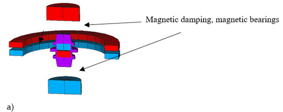
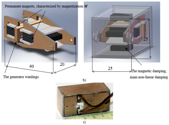
Figure 2.
The geometrical model of microgenerator (MG), (a) a primary version (magnetic bearing), (b) dimensions in mm for MG of BV, (c) experimental BV generator.
A swinging arrangement (BV, Figure 1 and Figure 2b,c) based on bearings with a minimum achievable damping rate lb has been proposed. The swinging arrangement was damped by a non-linear element-magnetic dampers at the extreme positions, Figure 2b,c. For maximum sensitivity, the electro-mechanical system was tuned to enter the resonance in the supposed frequency range fs of mechanical vibrations.
2. FEM Numerical Model
As mentioned in the principles and basics of the analytical design of the model [2,17,18,19], Figure 2, it is possible to describe electromagnetic field more generally with the FEM numerical model (1–11). The electromechanical vibrating harvester (34) works in special modes using resonances; its model includes nonlinearities and material nonlinearities depending on the temperature etc. As the first variant of the MG, the 3D structure with the application of magnetic damping elements was modeled and simulated. This variant did not used the cantilever beam, Figure 2a. Later, the second variant with cantilever beam swivel arrangement (BV) was also modeled a simulated.
The design of the numerical model was based on the reduced set of Maxwell equations in Heaviside’s notation for quasi-stationary cases of electromagnetic field. MG elements with a high degree of non-linearity and hysteresis (permanent magnet, ferromagnetic material of pole pieces, etc.) were used in the model and the MG worked in resonance mode, which is a therefore strongly nonlinear task [2]. The FEM model has taken into account all these criteria and the results of the analyzes were used to find sensitive parameters of the mathematical model. It was necessary to take into account the accuracy of the analysis and the parameters of the MG bond with the source of vibration.
In the numerical model of the discussed MG for quasi-stationary analysis, the effect of displacement currents (Equations (4a) and (6a)) was further retained. This displacement current effect was not used for the present MG model based on Faraday’s law of induction. It was taken in to account within analysis of another type MG with different parameters (higher vibration frequency) based on piezo-electric phenomenon. However, this piezo-electric generator is subject of other research. Therefore, the displacement current effect will not be used in the analysis of MG, Figure 2b,c. Next, a brief derivation of the numerical model for the tetrahedral, pentahedral and hexahedral elements of FEM will be briefly introduced. This model is using the Galerkin method of functional minimization with conversion to a mathematical problem. In the design of the basic model (Equation (12)) the relative motion of the magnetic field generated by the permanent magnet with magnetization M and the induction coil is considered as the source of excitation, Figure 1.
Analysis of MG model can be accomplished by numerical solution, FEM. The electromagnetic part of the model is based on the solution of reduced Maxwell equations in Heaviside notation
where H is the magnetic field intensity vector, B is the magnetic flux density vector, J is the current density vector.
where E is the electric field intensity vector, D is the electric flux density vector, ρe is the electric charge density, which is equal to zero for the considered MG and the area Ωs, Ωv ρeΩs, Ωv. Material relations are represented by the equations, whose respect the application of permanent magnets with magnetization M in both functional parts, the main part of the MG and their damping elements respectively.
where μ0 is vacuum permeability, μr is relative permeability of environment, μ = μrμ0, M is magnetization of permanent magnet, γ is specific conductivity of environment, ε0 is permittivity of vacuum, εr is relative permittivity, ε = ε0εr. The temporal changes of the electric and magnetic fields in the considered model of the MG, Figure 2, are negligible according to the expected parameters. That means, the relations (4b), (6b) are not respected in the proposed numerical model. Vector functions of electric and magnetic fields are expressed using scalar electric φe and vector magnetic potential A
The total current density from Equation (4a) J is superposed from the circuit’s excitation current density Jcirc and the current density from the eddy currents Jv. Movement is respected in the model by current density in both parts, electrically conductive parts and electrical windings of the MG respectively
The electromagnetic field model is formulated from Equations (1) to (10). Based on (1) and (10) is
For individual parts, Figure 1, of the model Ω holds Ω⊂Ωv∪Ωs, where Ωv is the region with dominant eddy currents, according to Equation (6a) Ωs is the region with known current density distribution Js. In the model under consideration:
Ωs ≡ Ωv
Then, Equation (11a) can be modified using formulas from (1) to (10) with respect to the source of the magnetic field or the damping elements based on permanent magnets that are represented by magnetization M, Figure 1:
where v is the velocity of the motion area Ω, s is the displacement vector, M is the magnetization vector and according to (4a) holds
From Equations (3a) and (3b), where the bond between the electric and magnetic field is captured
and is expressed with the help of used potentials relation
From the Equation (4b), where the distribution of the electric field is captured
The boundary and initial conditions will be determined as:
where n is a normal vector perpendicular to the boundary of the surface area Γ, Γi,j is the interface between the area i and the area j, ΓΩ is the interface at the outer edge of the area; the indexes i, j denotes for the quantities their belonging to the areas Ωi ≠ Ωj. Then the initial conditions are
The discretization of relations (12) to (14) can be accomplished by approximating the scalar electrical potential
where φe is the nodal value of the scalar electrical potential, W is the base function, Nφ is the number of nodes of the discretization network,
where S is the coordinate of the node, W is the base function, Ns is the number of nodes of the discretization elements,
where a is the node value of the vector magnetic potential, W is the base function, NA is the number of nodes of the discretization network. Applying the approximation (20) to (22) and the Galerkin method in relation (12) to (14) gives a semi-discrete solution for the region of Ωm model
The Equation (24) is modified by application of 2nd Green’s formula and Gauss’s theorem to expression
Respecting the boundary conditions of the problem according to the expressions (18), the relation (25) changes to
Applying the approximation (20) to (22) and the Galerkin method in relation (17a) gives a semi-discrete solution for the region of Ωm model
The expression (27) is modified by application of 2nd Green’s formula and Gauss’s theorem to expression
Substituting approximation functions, A, s, φε according to (20) to (22) into (26) and (28) gives a semi-discrete solution
Relation (29) can be rewritten to form
The simplified notation of the system of Equations (30) is
The expression is easy to rewrite to form
To simplify the calculation algorithm in the numerical part of the solution of the system of equations and its acceleration, the system (33) is converted to the form
The form of the coefficients is expressed in relations (30) and (31).
where i, j, k are the base vectors of the used Cartesian coordinate space. The algorithm for constructing matrices of coefficients (35) to (44) is simplified when the system of Equations (31) is rewritten to form
The coefficients of the system of the Equations (45) and (46) are expressed in the relations
The system of Equations (45) and (46) is written in the form
The procedure of quantification of the coefficients for tetrahedral, pentahedral and hexahedral element is described in detail [3].
The short description of the elements is shown in Figure 3, Figure 4 and Figure 5. The tetrahedral element in Figure 3 has a base function W
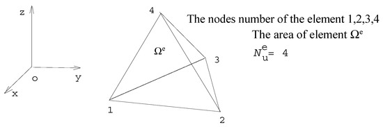
Figure 3.
The tetrahedral element and its symbolic description.
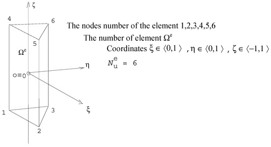
Figure 4.
The pentahedral element.
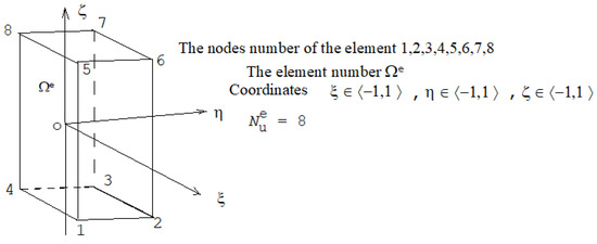
Figure 5.
The hexagonal element.
Make use of
where the indexes at x, y, z coordinates are local node numbers according to Figure 3. The coefficients of the function W can be expressed
where the indexes i, j, k, l change cyclically over a given interval. Index i is the natural number of the element function, indexes j, k, l are coordinate indexes of the element nodes. The coefficients of the model are for the tetrahedral element of Figure 3
where the indexes i, j are node numbers of the element e. If a pentahedral element is selected according to Figure 4 and the function W is displayed on it, then their writing at the selected local Cartesian coordinate system o,ξ,η,ζ is as follows:
and the gradient of the function W is expressed in the Cartesian coordinate system o, x, y, z
After the transformation of the function W into the global Cartesian coordinate system o, x, y, z from the local coordinate system o,ξ,η,ζ from the expressions (30) and (33) are the coefficients of the system of Equations (57). In them are
In the (77) relation, the derivative of the position vector Rp is represented by the following expression
the coordinates x, y, z and their derivatives according to the local coordinates ξ,η,ζ are expressed
When the hexahedral element from Figure 5 is selected, its base functions are written as
For the hexahedral element, the sizes of the coefficients from the set of Equations (57) are calculated from Equations (80)–(89) using the functions (90).
Integration in the relations (80) to (89) can be solved analytically. This method is difficult and time consuming. Avoiding the use of analytically expressed integrals in most cases will not significantly reduce the accuracy of the solution of the system of Equations (57). Another easier solution is to apply the Gaussian quadrature. Its form, usage and properties are known [3]. The coefficients of the system of Equations (57) are then calculated for a numerical solution
The number of integration points of the local coordinates for the tetrahedral element was chosen ng = mg = lg = 5. This number according to tests for accuracy and speed of quantification of quadrature relation fits the mathematical model. The expression of the auxiliary function L is identical to the function (58). By means of the L function, the coordinates of the integration points are determined according to the formulas (102) to (104) below.
Set values of the auxiliary function L and the weight function H for 5 selected points within the area Ωe are
The coordinates of the integration point are determined for the tetrahedral element
Six points of integration ng = mg = lg = 6 were chosen for the pentahedral element. The number corresponds to the required accuracy and speed of the quadrature calculation. The coordinates of the points are determined
Similarly, for a hexahedral element, where ng = mg = lg = 8. The coordinates of the point for calculating the quadrature according to (n102) to (n104) is expressed by the auxiliary function L
The electromagnetic part of the model of the task MG can be characterized by the expression (57). The description of the mechanical part of the model by means of the FEM is known for example from theses and works [1,2] and the system [21], then the electromechanically bounded equation is written in the form
where f is the vector of specific force, λ1, λ2 are auxiliary scalar functions. For the geometrical model, Figure 2, the external mechanical load was not considered. Such presumption will lead to f0 = 0. But, to respect the position of the MG in the earth’s gravitational field, with the acceleration g a static force, it was considered , where mg is the mass of the MG core, Vg is the volume of the MG core. The specific magnetic force fm is expressed as
There are valid boundary and initial conditions for the model, for example known [21]. Similar to the above, mentioned derivation of the electromagnetic part of the model, the coupled dynamical mechanical-electromagnetic model can be written in the form
and the corresponding semi-discrete model solution
After deriving and quantifying the corresponding coefficients of the system of equations, we obtain the overall FEM model with the corresponding matrices of coefficients K, M.
where is the column matrix of unknown magnetic vector potentials in the discretization network nodes, is a column matrix of unknown second derivatives of vector magnetic potentials over time in the discretization network nodes, {S} is a column matrix of unknown specific shift in nodes of the discretization network, {} is a column matrix of unknown second derivatives according to the time shift at the nodes of the discretization network, {t} is a column matrix of unknown temperature in nodes of discretization network, {} is a column matrix of unknown second derivatives according to time of unknown temperature in nodes of discretization network, is column matrix of unknown scalar electrical potentials in nodes of discretization network, column matrix of unknown second derivatives according to time of scalar electric potentials in nodes of discretization network, is column matrix of forces, is column matrix of vectors of tangential pressure components, is column matrix of vectors of normal pressure components is a column matrix of modulus vectors of specific deformation in temperature dependence of material.
Then the overall numerical FEM model of the electromechanical coupled task of the vibration MG is written as a system of equations
This problem can be solved in ANSYS [21] using programming tools and the APDL internal language.
The designed 3D model (112) was used to analyze and evaluate the transient excitation state of MG Figure 2a and Figure 6. Then, a steady state analysis of resonance and the corresponding electrical load RL was performed [18,19]. Sensitive parts of the MG model design have emerged from 3D analyzes and experiments. Due to the magnitude and amount of cumulative computations, absolutely not all details are given, but only the key details (the magnetic field in the MG core region). In order to find a suitable (optimal) direction of the magnetic arrangement solution, an accelerated 2D FEM model and a magneto-static field design were used, which in turn lead to maximizing the induced voltage u(t) in the winding of the MG coil.
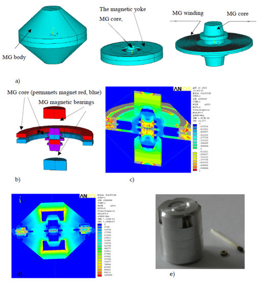
Figure 6.
The 3D model, analysis of the primary version MG (magnetic bearing) and MG realization, (a) geometrical model components, (b) conception, (c) field distribution of magnetic flux density module B [T], (d) field distribution of magnetic field intensity module H [A/m], (e) built MG sample prepared for test.
The 3D model was designed as the primary version of MG, Figure 6, which was not optimally arranged in the electro-mechanical conceptual design. It was solved both for start-up as a transient task and for the so-called steady-state regime in the resonant state by the model (112).
Given the previous experience with the complex analysis of the associated 3D model of the first version of MG, Figure 6, it became clear that critical part is the design of magnetic circuit of the MG (Figure 1 and Figure 8). For the chosen concept of the beam version of MG, Figure 7, only 2D static non-linear problem with hysteresis, Figure 8a was analyzed because of the higher speed of connected simulation. A conceptual solution of the magnetic circuit was proposed, using the results of performed analyzes, Figure 8b. Thus, a design with a maximum magnetic flux density B(t) and maximum amplitude of the electric voltage u(t) on the output of the MG’s winding has been achieved in a relatively rapid manner, Figure 7. According to these auxiliary FEM models and analyzes, the final concept of MG was designed, Figure 2b, Figure 7 and Figure 8.
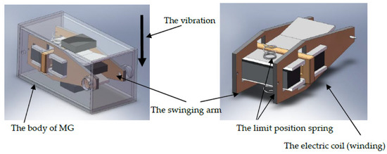
Figure 7.
The basic magnetic circuit of MG, structural design with magnetic damping in the limit position of the rocking arm.
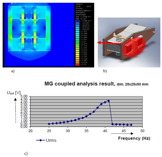
Figure 8.
The example of the beam MG model magnetic field analysis (a), 2D detailed distribution of the magnetic flux density module B [T] (b) the modeled part of generator, (c) coupled 3D model analysis result, output -root mean square (RMS) voltage Uout [V].
3. Modeling the MG
A free-arm system (BV) and its magnetic damping (non-linear) [19], Figure 7, has been designed.
Details of the MG evaluation of the analysis can be demonstrated for example in the magnetic field the distribution of the magnetic flux density module B [T] in Figure 8. The realized MG function sample, Figure 7 and Figure 8, was tested for the frequency range fs = 30–45Hz. Typical frequency dependencies of output voltage and output power of the MG are shown in Figure 9. The graph shows the effective value of the output power P_RMS and the effective electric voltage V_RMS at the MG’s winding output loaded by RL = 2.7KΩ at the vibration G = 0.5 g RMS.
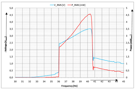
Figure 9.
The MG experimental measurement, root mean square (RMS) output voltage V_RMS, power P_RMS vs. frequency, frequency sweep with RL = 2.7kOhm, G = 0.5 g RMS, main operational resonant frequency.
4. Conclusions
The paper presents a detailed design of a numerical model of a FEM mini-generator for harvesting energy from vibrations within the range of G = 0.05 g − 0.08 g, for the frequency range of fs = 10–100 Hz, fmain = 36–41 Hz.
Based on the proposed beam version MG models and their analyses, evaluation of the parameters, qualitative conclusions were applied to design of the swinging arm of mini-generator, Figure 7. Some partial specific results from this systematic approach to generator design were published in theses and works [17,18,19]. This article describes a complete FEM numerical model that was used for vibration MG analysis. The results of the generator analysis were experimentally verified and subsequently utilized to build the functional MG.
A specific harvesting system for mechanical energy extraction was proposed. It utilizes the principle of transformation of propagating mechanical wave to electrical energy. The designed numerical model was implemented in ANSYS simulation software [21]. The simulated effective transformed mass and volume power densities of the generator are peff = 266 Wm- 3 and peffV = 0.31 Wkg−1 respectively.
The FEM model showed the key moment in the design of the first versions of MG concept and its design solutions. It also pointed out the key parameters of the model and directed the modifications of the MG’s equipment to the optimal solution of the harvester. An associated model (112), was able to detect the sensitive points of the task. This was proved by measurement results from experiments with the MG sample. FEM models of lower geometrical levels (2D) and simplified models (non-linear with hysteresis, etc.) were used as a necessary tool for quick estimation of the changes of design or concept changes.
Author Contributions
P.F. contributed to the theoretical section, numerical model, and experiments; he also wrote the paper; Z.S. conceived and designed the experiments; J.D. contributed to the optimization procedures; P.E., J.Z. and R.P. evaluated the experiments and graphics. All authors have read and agreed to the published version of the manuscript.
Funding
The research was financed by the BD 2020-2022, FEKT-S-20-6360, the infrastructure of the SIX Center was used.
Conflicts of Interest
The authors declare no conflict of interest. The founding sponsors had no role in the design of the study; in the collection, analyses, or interpretation of data; in the writing of the manuscript, and in the decision to publish the results.
References
- Stratton, J.A. Theory of Electromagnetic Field; Czech Version; SNTL: Praha, Czech Republic, 1961. [Google Scholar]
- Fiala, P. Vibration Generator Conception; Research report in Czech; DTEEE, Brno University of Technology: Brno, Czech Republic, 2003; p. 95. [Google Scholar]
- Jirků, T.; Fiala, P.; Kluge, M. Magnetic resonant harvesters and power management circuit for magnetic resonant harvesters. Microsyst. Technol. 2010, 16, 677–690. [Google Scholar] [CrossRef]
- Fiala, P.; Jirků, T. Analysis and Design of a Minigenerator, Progress in Electromagnetics 2008. In Proceedings of the PIERS 2014, Guangzhou, China, 25–28 August 2014; pp. 749–9450, ISBN 1559-9450. [Google Scholar]
- Madinei, H.; Khodaparast, H.H.; Adhikari, S.; Friswell, M. Design of MEMS piezoelectric harvesters with electrostatically adjustable resonance frequency. Mech. Syst. Signal Process. 2016, 81, 360–374. [Google Scholar] [CrossRef]
- Scapolan, M.; Tehrani, M.G.; Bonisoli, E. Energy harvesting using parametric resonant system due to time-varying damping. Mech. Syst. Signal Process. 2016, 79, 149–165. [Google Scholar] [CrossRef]
- Gatti, G.; Brennan, M.; Tehrani, M.; Thompson, D. Harvesting energy from the vibration of a passing train using a single-degree-of-freedom oscillator. Mech. Syst. Signal Process. 2016, 66, 785–792. [Google Scholar] [CrossRef]
- Davino, D.; Krejčí, P.; Pimenov, A.; Rachinskii, D.; Visone, C. Analysis of an operator-differential model for magnetostrictive energy harvesting. Commun. Nonlinear Sci. Numer. Simul. 2016, 39, 504–519. [Google Scholar] [CrossRef]
- Kulkarni, S.; Koukharenko, E.; Torah, R.; Tudor, J.; Beeby, S.; O’Donnell, T.; Roy, S.; Beeby, S. Design, fabrication and test of integrated micro-scale vibration-based electromagnetic generator. Sens. Actuators A Phys. 2008, 145, 336–342. [Google Scholar] [CrossRef]
- Beeby, S.P.; Torah, R.N.; Torah, M.J.; O’Donnell, T.; Saha, C.R.; Roy, S. A microelectromagnetic generator for vibration energy harvesting. J. Micromech. Microeng. 2007, 17, 1257–1265. [Google Scholar] [CrossRef]
- Zhu, D.; Roberts, S.; Tudor, M.J.; Beeby, S.P. Design and experimental characterization of a tunable vibration-based electromagnetic micro-generator. Sens. Actuators A Phys. 2010, 158, 284–293. [Google Scholar] [CrossRef]
- Wang, P.-H.; Dai, X.-H.; Fang, D.-M.; Zhao, X.-L. Design, fabrication and performance of a new vibration-based electromagnetic micro power generator. Microelectron. J. 2007, 38, 1175–1180. [Google Scholar] [CrossRef]
- Yang, J.; Yu, Q.; Zhao, J.; Zhao, N.; Wen, Y.; Li, P.; Qiu, J. Design and optimization of a bi-axial vibration-driven electromagnetic generator. J. Appl. Phys. 2014, 116, 114506. [Google Scholar] [CrossRef]
- Lee, B.-C.; Rahman, A.; Hyun, S.-H.; Chung, G.-S. Low frequency driven electromagnetic energy harvester for self-powered system. Smart Mater. Struct. 2012, 21, 125024. [Google Scholar] [CrossRef]
- Zhu, D.; Tudor, M.J.; Beeby, S.P. Strategies for increasing the operating frequency range of vibration energy harvesters. J. Meas. Sci. Technol. 2010, 21, 22001. [Google Scholar] [CrossRef]
- El-Hami, M.; Glynne-Jones, P.; White, N.; Hill, M.; Beeby, S.; James, E.; Brown, A.; Ross, J. Design and fabrication of a new vibration-based electromechanical power generator. Sens. Actuators A Phys. 2001, 92, 335–342. [Google Scholar] [CrossRef]
- Fiala, P.; Szabo, Z.; Marcon, P.; Roubal, Z. Mini-and Microgenerators Applicable in the MEMS Technology, Smart Sensors, Actuators, and MEMS VIII. Proc. SPIE 2017, 10246, 1–8. [Google Scholar] [CrossRef]
- Szabo, Z.; Fiala, P.; Dohnal, P. Magnetic circuit modifications in resonant vibration harvesters. Mech. Syst. Signal Process. 2018, 99, 832–845. [Google Scholar] [CrossRef]
- Szabó, Z.; Fiala, P.; Zukal, J.; Dědková, J.; Dohnal, P. Optimal Structural Design of a Magnetic Circuit for Vibration Harvesters Applicable in MEMS. Symmetry 2020, 12, 110. [Google Scholar] [CrossRef]
- Figlus, T.; Kozioł, M.; Kuczyński, L. The effect of selected operational factors on the vibroactivity of upper gearbox housings made of composite materials. Sensors (Switzerland) 2019, 19, 4240. [Google Scholar] [CrossRef] [PubMed]
- ANSYS Users Manual, (1991–2020). USA. Available online: www.ansys.com (accessed on 1 July 2018).


© 2020 by the authors. Licensee MDPI, Basel, Switzerland. This article is an open access article distributed under the terms and conditions of the Creative Commons Attribution (CC BY) license (http://creativecommons.org/licenses/by/4.0/).