Selection of the Informative Frequency Band in a Bearing Fault Diagnosis in the Presence of Non-Gaussian Noise—Comparison of Recently Developed Methods

Abstract

The vibration signals acquired on machines usually have complex spectral structure. As the signal of interest (SOI) is weak (especially at an early stage of damage) and covers some frequency range (around structural resonance), it requires its extraction from a raw observation. Until now, most of the techniques assumed the presence of Gaussian noise. Unfortunately, there are cases when the non-informative part of the signal (considered as the noise) is non-Gaussian due to the random disturbances or nature of the process executed by the machine. Thus, the problem can be formulated as the extraction of the SOI from the non-Gaussian noise. Recently this problem has been recognized by several authors and some new ideas have been developed. In this paper, we would like to compare these techniques for benchmark signals (Gaussian noise, cyclic impulsive signals, non-cyclic impulsive signals with random amplitudes and locations of impulses and a mixture of all of them). Our analysis will cover spectral kurtosis, kurtogram, stability index (Alpha selector), conditional variance-based selector, spectral Gini index, spectral smoothness index and infogram. Finally, a discussion on the efficiency of each method is provided.

1. Introduction

The problem of bearings local damage detection is widely discussed in the literature [1,2,3,4]. In the case of constant speed, the task is defined as the detection of the periodic impulsive signals. The vibration under time-varying speed requires special treatment, see [5,6], and will not be considered in this paper. The most popular approach is the envelope analysis and detection of fault frequencies in the spectrum of the envelope for a pre-filtered signal. The modified versions of the envelope are also known, e.g., squared envelope spectrum (SES) [2,7], log-envelope spectrum (LES) [8,9]. The filtration of a raw signal is used to select its informative part and avoid other spectral content not related to the local damage. Depending on the complexity of the structure of the signal one may use simple band-pass filtering, advanced decomposition via Empirical Mode Decomposition (EMD) [10,11] or wavelet transform [12,13,14]. An optimal solution has been proposed by using Wiener filtering [15]. The filter coefficients could be optimized by the genetic algorithm proposed in [16]. The most popular approach is based on the spectral kurtosis as an informative frequency band (IFB) selector (filter characteristic). The kurtosis value is calculated for sub-signal at some narrow frequency band. As kurtosis is sensitive to outliers [17], one can select impulsive content at a given narrow frequency band and filter out other components. Kurtosis is the most intuitive statistic commonly used for machine diagnostics [18]. It has plenty of variations and extensions, e.g., the kurtogram [19]—which is a colored map, where the depth of the color values is proportional to the kurtosis value. Obuchowski showed that other statistics could also be used in such context [20]. Recently, many techniques for searching for optimal frequency band selection have appeared [21].

In the literature, one can also find methods which are based on the cyclostationary approach. Obviously, these algorithms are dedicated to the cyclic behavior identification for the real signals. In the classical approach of cyclostationary-based techniques the assumption of Gaussian noise is taken under consideration [7,9,22,23,24,25,26]. However, one can find the papers where the algorithms for the signals with non-Gaussian noise are proposed [27,28,29,30,31,32,33,34,35,36,37,38]. We refer also to the recent paper, where the new definition of the cyclostationary non-Gaussian signal is given, see [27] for more details. However, in this paper we do not consider the cyclostationary-based methods.

One can also find other approaches for the IFB selection based on artificial intelligence [39,40,41]. However, there is still a need for new approaches that allow us to consistently handle restrictions linked to the amount of available data, specific type of noise, work specifications of the tested machine, etc.

The idea of the paper is not to introduce a new technique which outperforms other methods for signals with the specific behavior, but to demonstrate the advantages and limitations of the selected algorithms. In many papers authors refer to other existing techniques to compare performance. However, due to lack of space in research papers, a novel technique can be compared to one or two other techniques for some specific signal, without a deep understanding of properties/limitations of each method. It makes real comparison difficult. Thus, the main goal of the paper is to compare the recently proposed methods for the IFB selection. The paper provides a comparative study of different methods used for local damage detection for real-life inspired benchmark signals (Gaussian White Noise, cyclic impulsive signals, non-cyclic impulsive signals with random amplitudes and locations of impulses and a mixture of all of them). The most complicated simulated signal considered in this paper, apart from the background noise, contains the non-cyclic impulses which are not informative. According to our knowledge, this kind of signal was not considered in the context of the comparison of different techniques and thus in our opinion, such a comparison is worthy to demonstrate.

The signals with non-cyclic impulsive behavior we observe in the real environment. One of the examples is the crushing machine [42] used in mines. During the operation of the machine (the crushing process), apart from the background noise (which is often assumed to be Gaussian White Noise) large observations appear in the vibration signal, due to the nature of the machine’s work. Moreover, in the case of local damage, additional cyclic impulses are hidden in the noise. In this case, the detection of local damage is very difficult. In this paper, we have used simulated signal with specific properties (cyclic, non-cyclic impulses and noise components). The use of a generic model has allowed presenting the problem and test algorithms for various cases.

The problem can be formulated as the extraction of the SOI from the Gaussian and non-Gaussian noise. Recently the last, more demanding problem has been recognized by several authors and some new ideas have been developed [21,42,43,44].

Our analysis will cover spectral kurtosis [45], kurtogram [19], stability index (Alpha selector) [46], spectral Gini selector [47], spectral smoothness index [17], infogram [48] and conditional variance-based selector [49].

The first six methods were considered in the literature as the most effective and classical ones in the problem of local damage detection. In our recent research [49], we have utilized the statistic called the conditional variance statistic and proposed a new algorithm for local damage detection which seems to be applicable when the background noise is contaminated by the non-cyclic large impulses. In the paper [49], we have indicated the limitations of the proposed method and proved its effectiveness, especially when the ratio of the amplitudes of non-cyclic to cyclic impulses is large. In the current paper, which can be considered as the extension of our previous research, we demonstrate that the results obtained for the conditional variance-based selector are superior with respect to the results based on the mentioned other algorithms.

The rest of the paper is organized as follows. In Section 2, we remind the reader of the definitions of seven considered selectors for local damage detection. Next, in Section 3 we give a short description of the model of the simulated signal and comparatively study the results for the considered algorithms. At the end of this section the efficiency of the analyzed selectors has been tested on real data. The last section concludes the paper.

2. Informative Frequency Band Selectors

Real vibration signals are typically a mixture of sources with a complex spectral structure. The signal of interest is hidden in such a mixture. To improve the Signal-to-Noise Ratio, before demodulation (envelope analysis), an extraction of the SOI is needed. According to the literature, damage signature covers some frequency range around structural resonance [18]. To find the informative frequency band (IFB), some statistical indicators for impulsiveness detection are used. In this section, selected statistics are recalled.

2.1. Kurtosis

The kurtosis statistic is the most known impulsive measure in the probability and statistical theory, see [50]. It gives knowledge about the non-Gaussianity of the signal (for the Gaussian distribution the statistic is equal to 0) or in other words about the impulsiveness of the signal. The kurtosis for the vector $x=(x_1,x_2,\dots ,x_N)$ is defined as follows [51]:

$$\begin{array}{c}\hfill \widehat{K}\left(x\right)=\frac{\frac{1}{N}{\sum }_{i=1}^N{\left(x_i-\overline{x}\right)}^4}{{\left(\frac{1}{N}{\sum }_{i=1}^N{\left(x_i-\overline{x}\right)}^2\right)}^2}-3,\end{array}$$

(1)

where $\overline{x}$ is the sample mean and N is the sample length. It is the most frequently used sparsity index in the diagnosis of bearing faults [45,52]. In our approach, we apply the kurtosis not to the raw signal, but to its time-frequency representation. The time-frequency representation of the signal is widely used because it gives the temporal and spectral content simultaneously and provides much more information about data than the one-dimensional representation in the time domain. The signal decomposition can be performed by the short-time Fourier transform (STFT) or many other techniques (Wavelets, Wigner, EMD, etc.), see, e.g., [53]. In our case, the STFT is applied. The interpretation of the STFT-based map is intuitive—it describes the energy flow in time for some narrow frequency band, i.e., sub-signal [18,20,46,49,54]. The spectrogram has some limitations. It is well known that selection of the window, its length, overlap size, etc., is a compromise between time and frequency domain resolution and strongly depends on the signal. By trials and error, we have found the “optimal” solution for the given signal. To calculate the STFT we assume 512 sampling points to calculate the discrete Fourier transform and Hamming windowing for window size 256. The number of samples of overlap between adjoining segments has been set on $\lfloor 85\%·\mathrm{window}\rfloor$.

The usage of the spectral kurtosis has been proposed in the rotating machinery diagnosis by Antoni [45]. After time-frequency signal decomposition the statistic $\widehat{K}(·)$ applied to the individual frequency band $f_i$: $\widehat{K}\left(f_i\right)$ is called spectral kurtosis.

One may find the usage of the filter bank for the signal decomposition, e.g., $1/3$-binary tree structure [19]. Then the statistic $\widehat{K}(·)$ can be applied to the real part of the envelope of the signal at frequency $f_i$. The representation of the spectral kurtosis in the $(f,\Delta f)$ plane is called a kurtogram [19].

Currently, it is known that methods which are based on the kurtosis statistic have some limitations. The value of the kurtosis decreases when the repetition rate of the impulses increases. If the cyclic impulses become so frequent that they overlap over each other, then the kurtosis vanishes [55]. On the other hand, when the outliers (non-cyclic impulses) are observed in the recorded signal then the kurtosis takes maximal value. This issue was addressed in [3] where the authors proposed an interesting alternative, namely the protrugram. It is based on the kurtosis of the envelope spectrum rather than the signal. However, despite its advantages, the protrugram has some limitations as well. It considers only the periodicity without scoring the impulsive behaviour. What is more, in the case of outliers its envelope spectrum distorts, thus the protrugram’s results can be misleading.

2.2. Stability Index

The class of $\alpha$-Stable distributions is known as an extension of the classical Gaussian distribution, see [56]. One of the distribution’s parameters is the stability index $\alpha \in (0,2]$, which indicates the distance from the Gaussian distribution. In other words, this parameter indicates how impulsive is the distribution. For the $\alpha =2$ the $\alpha$-distribution simplifies to the Gaussian distribution with some parameters $\mu ,\sigma$. If the $\alpha$ tends to 0, then the examined distribution becomes more impulsive (the values of the outliers significantly increase). The $\alpha$-stable distribution is defined by the characteristic function [56], which is as follows:

$$\mathbb{E}[expi\theta X]={\varphi }_X\left(\theta \right)=\left\{\begin{array}{cc}{e}^{-{\sigma }^{\alpha }{\left|\theta \right|}^{\alpha }\left\{1-i\beta \mathrm{sign}\left(\theta \right)tan\left(\pi \alpha /2\right)\right\}+i\mu \theta },\hfill & \alpha \ne 1,\hfill \\ e^{-\sigma \left|\theta \right|\{1+i\beta \mathrm{sign}\left(\theta \right)\frac{2}{\pi }log\left(\right|\theta \left|\right\}+i\mu \theta },\hfill & \alpha =1.\hfill \end{array}\right.$$

The parameters $\sigma >0$, $\beta \in [-1,1]$, and $\mu \in \mathbb{R}$ are the scale, skeweness and shift parameters respectively. To estimate the parameter $\alpha$ from the $\alpha$-stable distribution one can use the following definition, adapted from the McCulloch method [57]:

$$\begin{array}{c}\hfill \widehat{\alpha }\left(x\right)=\psi ({\widehat{v}}_{\alpha },{\widehat{v}}_{\beta }),{\widehat{v}}_{\alpha }=\frac{{\widehat{x}}_{.95}-{\widehat{x}}_{.05}}{{\widehat{x}}_{.75}-{\widehat{x}}_{.25}},{\widehat{v}}_{\beta }=\frac{{\widehat{x}}_{.95}-{\widehat{x}}_{.05}-2{\widehat{x}}_{.5}}{{\widehat{x}}_{.95}-{\widehat{x}}_{.05}},\end{array}$$

(2)

where $\widehat{x_q}$ is the sample quantile of order q based on the vector $x=(x_1,\cdots ,x_N)$. The parameter $\widehat{\alpha }$ is obtained by the linear interpolation $\psi (·,·)$ of the $v_{\alpha }$ and $v_{\beta }$ is based on the McCulloch tabulation of the function $\psi (·,·)$, see Table III in [57].

The usage of the parameter $\alpha$ has been presented in [46,58], where the Alpha selector has been defined as 2-$\widehat{\alpha }$ and applied to the spectral frequency $f_i$: $\widehat{\alpha }\left(f_i\right)$ after time-frequency signal decomposition performed by the short-time Fourier transform (STFT). The Alpha selector was found as an effective tool for the IFB selection in the bearing fault diagnostics. As it was mentioned, if the amplitude of the impulses in the examined data distribution increase then the $\widehat{\alpha }$ parameter tends to 0 and Alpha selector increases.

2.3. Gini Index

Gini index was originally proposed in economics [59] to measure the inequality of wealth and it has been recognized as a sparsity measure. It was also applied in others area, e.g., in the speech signal processing [60]. Recently Miao et al. [47] replaced kurtosis in the framework of a $1/3$-binary tree filter bank (i.e., kurtogram) with the Gini index used to quantify the envelope of filtered signals for extraction of bearing fault signals from a vibration mixture. The results experimentally demonstrated the effectiveness of the spectral Gini index for characterizing repetitive transients caused by bearing defects. Another application of the spectral Gini index for bearing fault diagnosis can be found in the recent work of Wang et al. [61]. The Gini index of signal $x=(x_1,\cdots ,x_N)$ is defined as:

$$\begin{array}{c}\hfill \widehat{G}\left(x\right)=1-2\sum _{i=1}^N\frac{x_{\left(i\right)}}{{∥x∥}_1}\left(\frac{N-i+\frac{1}{2}}{N}\right),\end{array}$$

(3)

where numbers $\left(1\right),\left(2\right),\left(3\right),\cdots ,\left(N\right)$ are the new indices after the sorting operation of vector x and ${\parallel ·\parallel }_p$ is the p-norm of vector x: ${\parallel \mathbf{x}\parallel }_p=\left(\right|x_1{|}^p+|x_2{|}^p+\dots +{\left|x_N\right|}^p{)}^{1/p}$.

In general, the Gini index equal to 0 represents ideal energy equality, that is, each component has the same share, while the Gini index equal to 1 reflects the maximum energy inequality, which means that all energy belongs to one component. The characteristics of this inequality indicator are discussed in [62]. In the recent work of Wong [17] one may find that the Gini index is less sensitive to outlier values than the spectral kurtosis. The IFB selector based on the Gini index is obtained by simply replacing the kurtosis statistic in the kurtogram with the Gini index.

2.4. Smoothness Index

Similar functionality to the kurtosis presents the smoothness index introduced by Bazchalooi and Liang [63]. It has been recognized by Wang [17] as another attractive and important statistical parameter to characterize transient states. The estimator of the smoothness index S for the vector $x=(x_1,\cdots ,x_N)$ is defined as follows:

$$\begin{array}{c}\hfill \widehat{S}\left(x\right)=\frac{\frac{1}{N}{∥x∥}_1}{{\left({\prod }_{i=1}^N{x}_i\right)}^{\frac{1}{N}}}-exp\left(\gamma \right),\end{array}$$

(4)

where $\gamma$ is the Euler–Mascheroni constant $0.5772156649$. The spectral smoothness index is defined as the ratio of the geometric mean and the arithmetic mean of the wavelet coefficient moduli of the vibration signal. The spectral smoothness selector is obtained by simply replacing the kurtosis statistic in the kurtogram with the smoothness index defined in Equation (4).

Thanks to the great efforts made by Wang [17], it has been mathematically proven that the spectral kurtosis, spectral Gini index and spectral smoothness index are sensitive to outliers. However, spectral smoothness index and spectral Gini index are less sensitive to outliers than spectral kurtosis.

2.5. Conditional Variance Statistic

The conditional variance statistic is described in details in [49]. It originates from the statistical phenomenon commonly referred to as the $20/60/20$ Rule [64,65]. It is based on the conditional variance measurement. This rule says that if the population is divided into three groups, according to some arbitrary reference criterion, (e.g., $20\%$ of the smallest, $60\%$ of the middle and $20\%$ of the largest values), this particular relationship often means some kind of balance. In the paper [64], the mathematical illustration that justifies this rule in many real-world situations has been demonstrated. It has been also shown that for any population that can be described by a multidimensional normal vector, this fixed ratio leads to a global equilibrium state. The conditional variance statistic used in [49] for the bearing fault diagnosis is defined as follows:

$$\begin{array}{c}\hfill {\widehat{C}}_7\left(x\right):={\left(\frac{{\widehat{\sigma }}_{A_3}^2-{\widehat{\sigma }}_{A_4}^2}{\widehat{\sigma }}+\frac{{\widehat{\sigma }}_{A_5}^2-{\widehat{\sigma }}_{A_4}^2}{\widehat{\sigma }}\right)}^2\sqrt{N}.\end{array}$$

(5)

The lower index 7 in the statistic $C_7(·)$ refers to the amount of the partitions $A_i$ into which the distribution of the vector $x=(x_1,\dots ,x_N)$ has been divided. Whereas ${\widehat{\sigma }}_{A_i}$ denotes the estimator of the standard deviation ${\sigma }_{A_i}$ in the given set $A_i$. The main property of divisions $A_i$ is that their variances are equal. More specifically, for partitioning on 7 subsets the estimators of $A_i$ are defined as follows [65]:

$$\begin{array}{cc}\hfill {\widehat{A}}_1& :=(-\infty ,{\widehat{x}}_{.004}],\hfill \\ \hfill {\widehat{A}}_2& :=({\widehat{x}}_{.004},{\widehat{x}}_{.062}],\hfill \\ \hfill {\widehat{A}}_3& :=({\widehat{x}}_{.062},{\widehat{x}}_{.308}],\hfill \\ \hfill {\widehat{A}}_4& :=({\widehat{x}}_{.308},{\widehat{x}}_{.692}],\hfill \\ \hfill {\widehat{A}}_5& :=({\widehat{x}}_{.692},{\widehat{x}}_{.938}],\hfill \\ \hfill {\widehat{A}}_6& :=({\widehat{x}}_{.938},{\widehat{x}}_{.996}],\hfill \\ \hfill {\widehat{A}}_7& :=({\widehat{x}}_{.996},\infty ),\hfill \end{array}$$

where ${\widehat{x}}_q$ is the empirical quantile of order q calculated for vector x. Assuming the Gaussian distribution the following equation is fulfilled [65]:

$${\sigma }_{A_1}^2={\sigma }_{A_2}^2={\sigma }_{A_3}^2={\sigma }_{A_4}^2={\sigma }_{A_5}^2={\sigma }_{A_6}^2={\sigma }_{A_7}^2.$$

(6)

As noted in [64], the condition (6) creates a dispersion balance for the conditional populations and a different number of partitioning sets could be considered.

After time-frequency signal decomposition the estimator ${\widehat{C}}_7(·)$ applied to the individual frequency band $f_i$: ${\widehat{C}}_7\left(f_i\right)$ is called conditional variance-based selector (CVB selector). The CVB selector is able to distinguish different impulses occurring based on the distribution of their amplitudes [49]. However, it does not take into account the periodicity of the impulses. It is a general problem for all listed selectors demonstrated above.

2.6. Negentropy

Entropy is a general concept that measures the disorder in a system. In the thermodynamic theory, the strength of the energy is uniform over the whole system (called the state of equilibrium) and it is characterized by constant temperature and maximum entropy. In the signal processing terminology, it means that the system is stationary. One can find the usage of the entropy measure in [66,67].

Negentropy, the opposite of entropy, was proposed by Antoni [48] as a measure of impulsiveness, in the time domain (in SE—Squared Envelope) and in the frequency domain (in SES—Squared Envelope Spectrum), which are additive and their average was proposed as a fault (impulsive and cyclical impulses) detection tool. The associated quantities displayed as functions of the frequency and frequency resolutions form “SE infogram”, “SES infogram” and “average infogram” [48]. The estimator of negentropy for the vector $x=(x_1,\dots ,x_N)$ is defined as follows:

$$\begin{array}{c}\hfill \widehat{I}\left(x\right)=\frac{1}{N}\sum _{i=1}^N\left(\frac{{x_i}^2}{\frac{1}{N}{\sum }_{i=1}^N{x}_i}ln\frac{{x_i}^2}{\frac{1}{N}{\sum }_{i=1}^N{x}_i}\right).\end{array}$$

(7)

In order to obtain the $SE$ and $SES$ infograms ($I_{SE}$, $I_{SES}$) the vector x in the Equation (7) has to be substituted by the corresponding $SE$, or in case of the $SES$ infogram by $\left|SES\right|$, of the filtered signal for the tested frequency band f +/- $\Delta f$. Then, using the formula (8) the average infogram (called infogram) has been proposed [48]:

$$\begin{array}{c}\hfill \Delta I(f,\Delta f)=\frac{I_{SE}+I_{SES}}{2}.\end{array}$$

(8)

Infogram considers both specific features of repetitive transient states: impulsiveness in the time and frequency domains. Hence, it distinguishes oneself among the other selectors. However, the energy from the envelope and the energy from the envelope spectrum have no upper bounds and their scales may differ significantly, therefore the average of both can be exposed to scoring the result, for which the scale is larger.

3. Data Analysis

3.1. Simulated Signals Description

In order to verify the selectors’ efficiency, we simulated four different types of the signals: $s_1,s_2,s_3$ and $s_4$. The first of the signal $s_1$ is the Gaussian White Noise: $s_1=N\left(t\right)$, which corresponds to the bearing vibration in a healthy condition, see Figure 1a. In such a case, we expect that any of the IFB selectors respond significantly. The signal’s frequency is $\mathrm{25,000}$ Hz and its length is 1 s. Signal $s_2$ corresponds to the locally damaged bearing vibration and it is defined as follows:

$$\begin{array}{c}\hfill s_2=ACI·gauspuls(t_0,f{c}_0,b{w}_0)+s_1,\end{array}$$

(9)

where $gauspuls(t,fc,bw)$ is a unity-amplitude Gaussian RF (radio-frequency) pulse at the times indicated in array t, with a center frequency $fc$ in hertz and a fractional bandwidth $bw$. $ACI$ is the amplitude of the cyclic impulses ($ACI=3$), $f{c}_0$ is set to 2500 Hz and the frequency modulation of cyclic impulses is equal to 30 Hz. Simulated signal $s_2$ has been presented in Figure 1b.

Signal $s_3$ imitates the bearing operation of the loaded machine in a healthy condition and it is defined as follows:

$$\begin{array}{c}\hfill s_3=ANCI·gauspuls(t_1,f{c}_1,b{w}_1),\end{array}$$

(10)

where $ANCI$ is the amplitude of the non-cyclic impulses ($ANCI=30$), $t_1$ is the location of the non-cyclic impulses, which has the uniform distribution. Signal $s_3$ has been presented in Figure 1c. The last of the signal is the mixture of previously mentioned, namely, it is defined as follows:

$$s_4=s_2+s_3.$$

It imitates the bearing vibrations in case of the loaded machine operating in the unhealthy condition of bearing, see Figure 1d.

3.2. Results for the Simulated Data

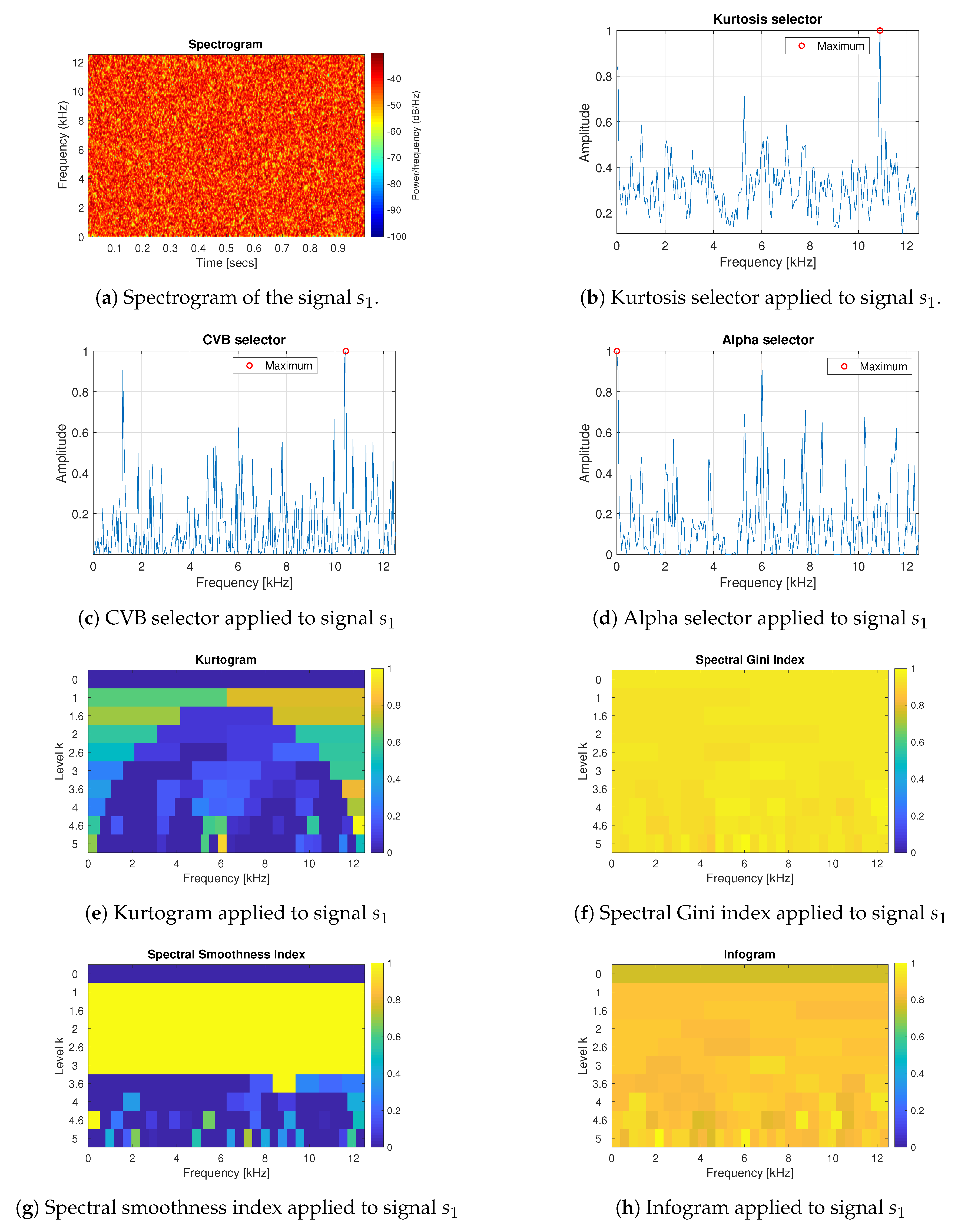
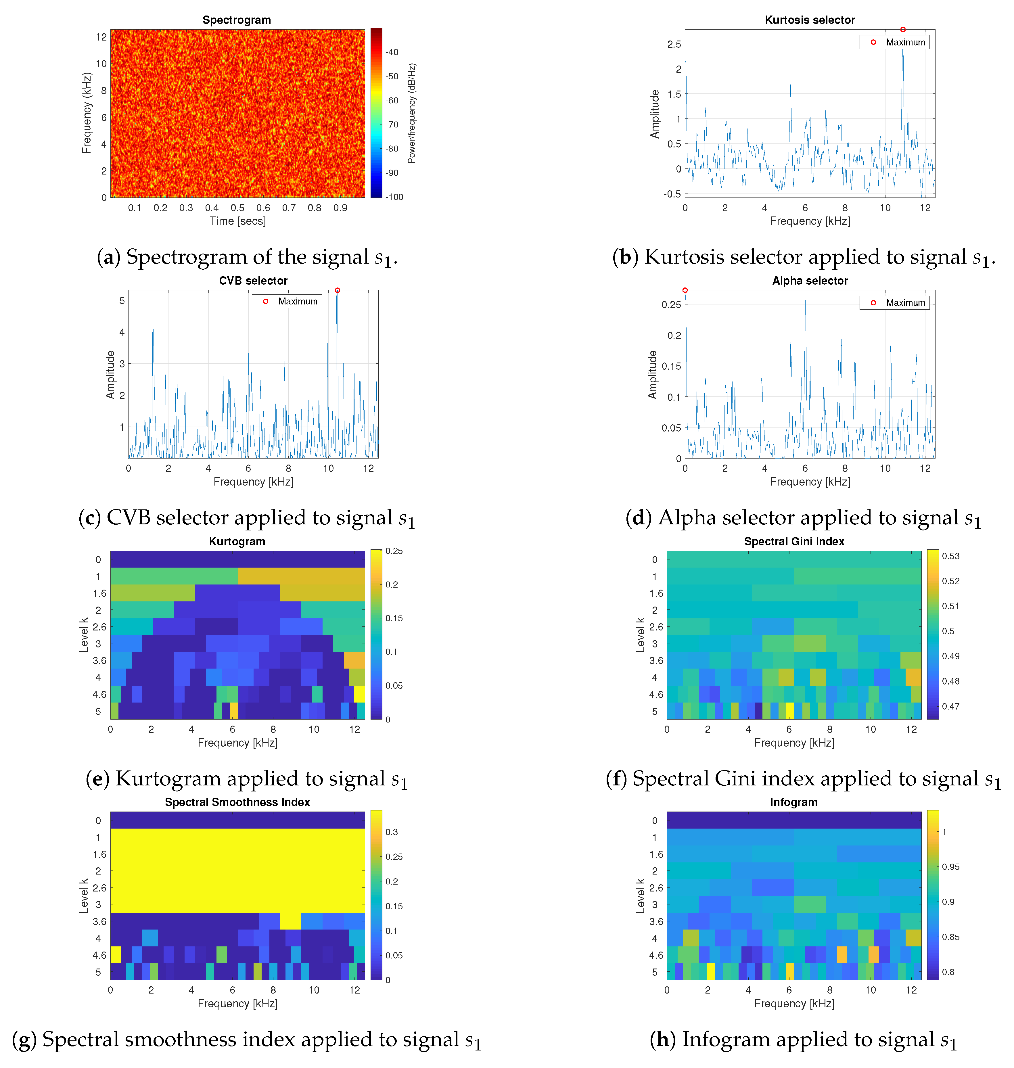
In this section, the comparative results are presented for simulated data. For each of the previously defined signals $s_1,s_2,s_3$ and $s_4$ the selectors presented above have been applied. In Figure 2a the spectrogram of the signal $s_1$ has been presented. The signal is the Gaussian White Noise, so it is not impulsive and not periodic.

As one can see in Figure 2b–h, if the signal contains only Gaussian noise, all of the considered techniques (kurtosis, CVB, Alpha selectors, spectral Gini and spectral smoothness indexes), as well as the infogram, have relatively small amplitudes and do not indicate the informative frequency band, as expected. There is no frequency band within 256 tested, which significantly stands out from the others (in Figure 2e–h see the last 5th level of the decomposition in the $1/3$-binary tree structure). However, one can note that the spectral smoothness index takes maximum value within all frequency range up to the 3rd level of the decomposition. It is related to the decomposition of the signal through the filter bank (for each decomposition level the signal is shorter). It changes the length of the vector, which is tested by the given statistic. As one can see in Equation (4), in the denominator of the statistic’s definition there is the product of the vector’s components. Hence, if the value of the vector components are relatively small in the absolute values, then the spectral smoothness index tends to infinite (marked in yellow in Figure 2g). One can notice that this happen especially in case of the long vectors with small values, here up to the 3rd level of the decomposition.

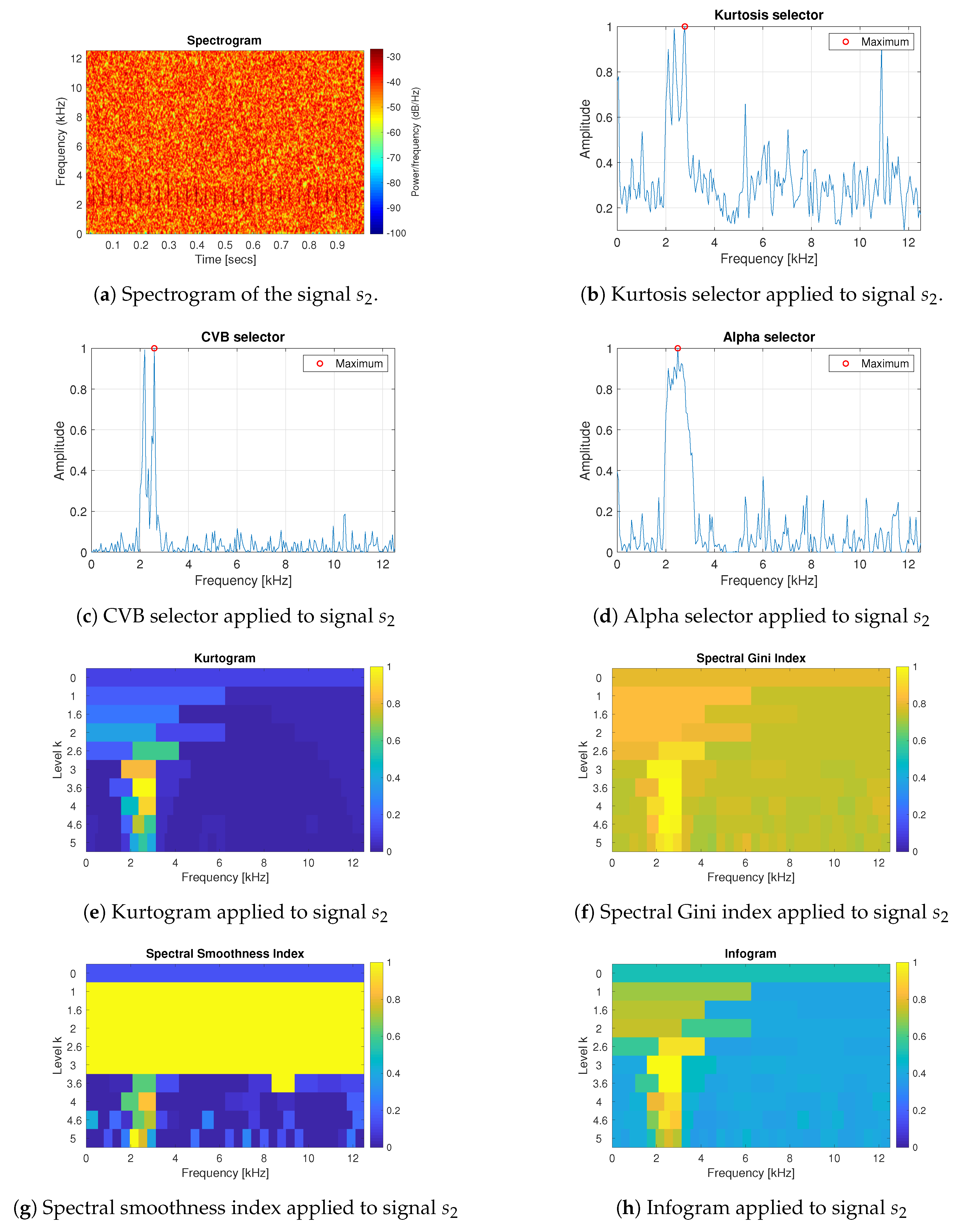
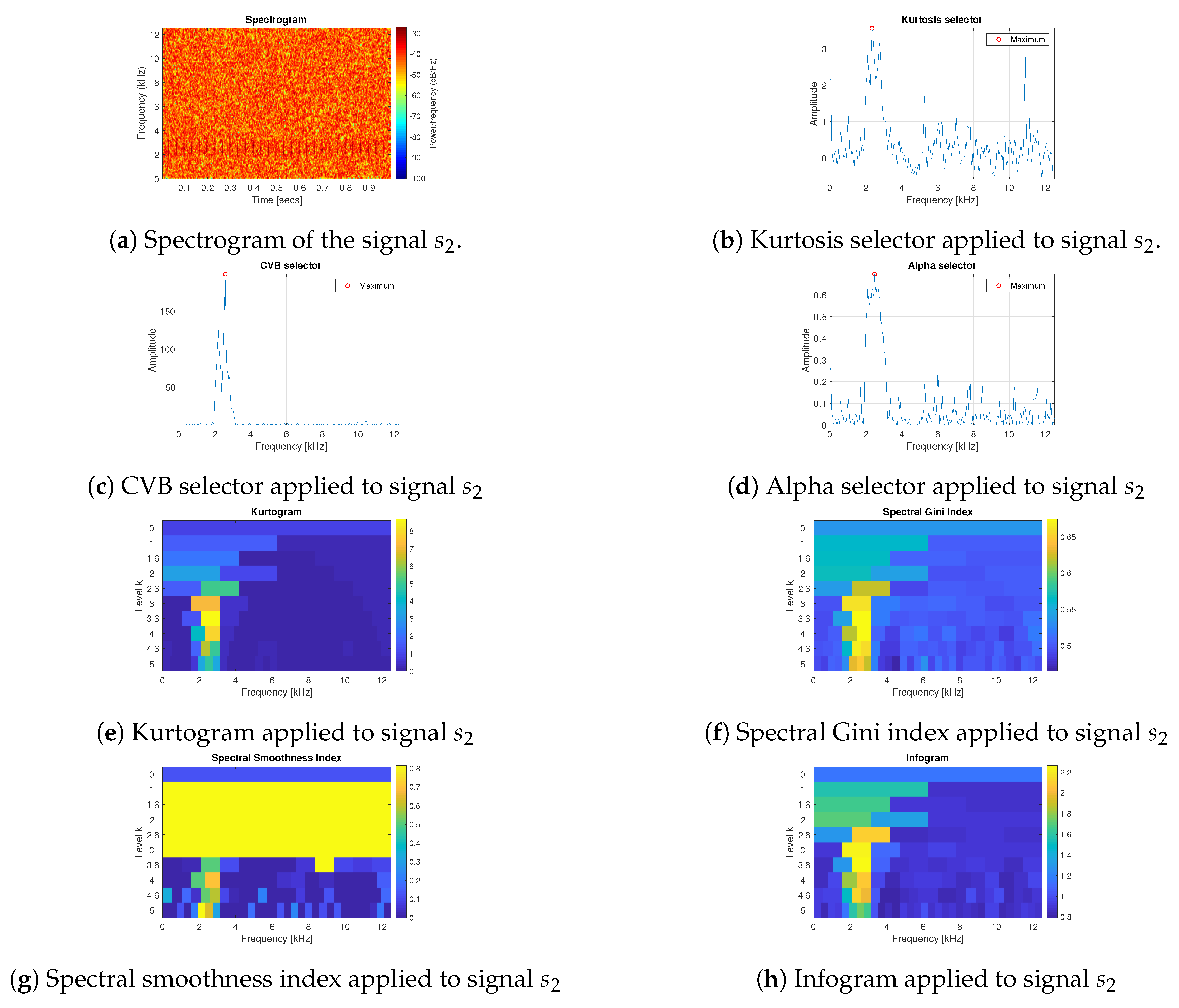
For the cyclic impulsive signal, described in Equation (9), we expect that the techniques point out the IFB between 2–3 kHz (the centre frequency is set on 2500 Hz).

As one can see in Figure 3b–h, for signal $s_2$ all techniques work well but the results for the CVB selector seem to be most unequivocal. The value of the CVB selector in the range of the IFB is significantly higher than for other frequency bins. If the cyclic impulses will have higher amplitudes then their variance will increase and the value of the CVB statistic will increase as well. For the tested signal, the $ACI$ parameter determines the amplitude of the cyclic impulses and it is assumed that $ACI$ is equal to 3. It means that the cyclic impulses are almost fully hidden in the Gaussian noise $ACI\le 3\sigma +\mu$, where $\sigma =1$ and $\mu =0$.

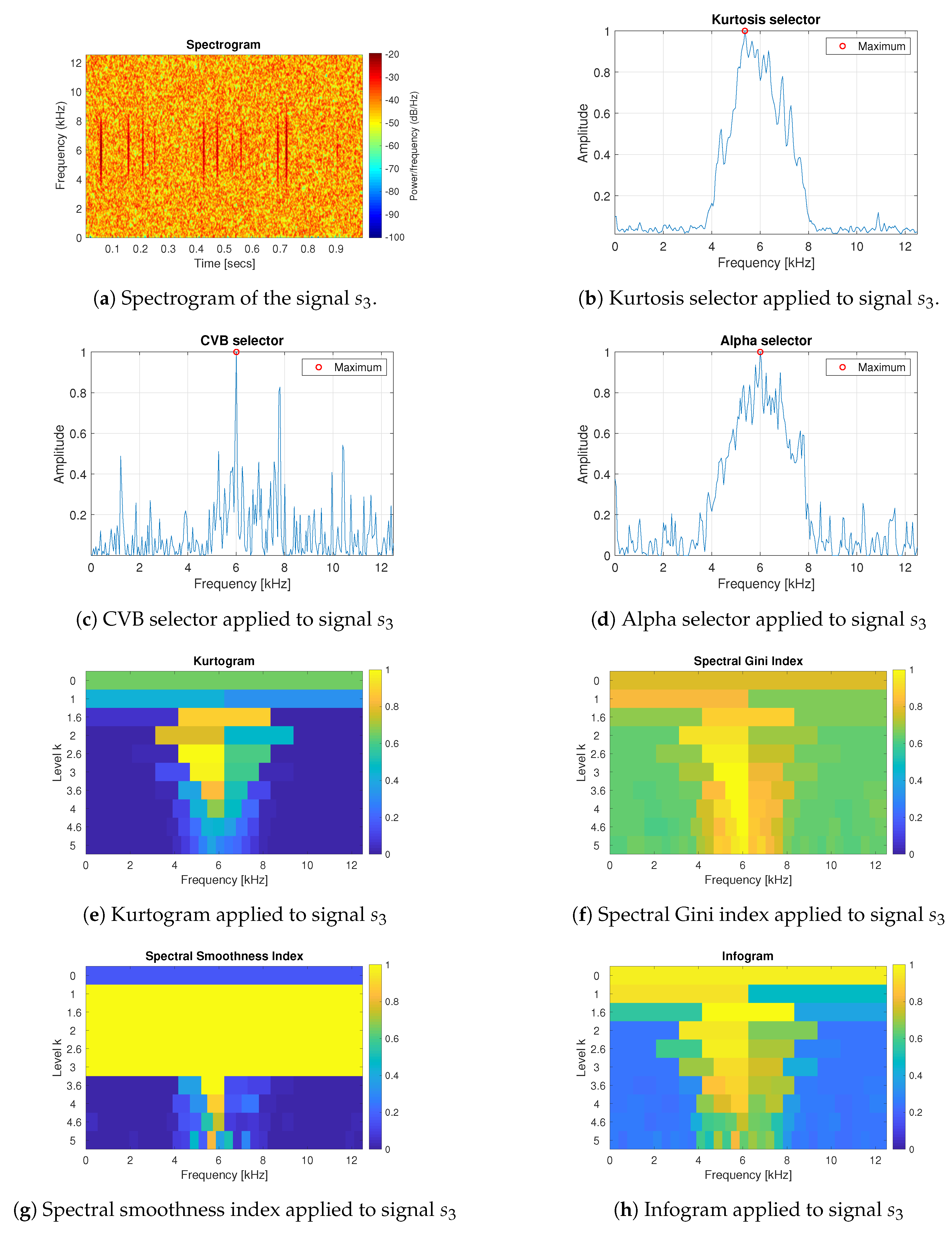
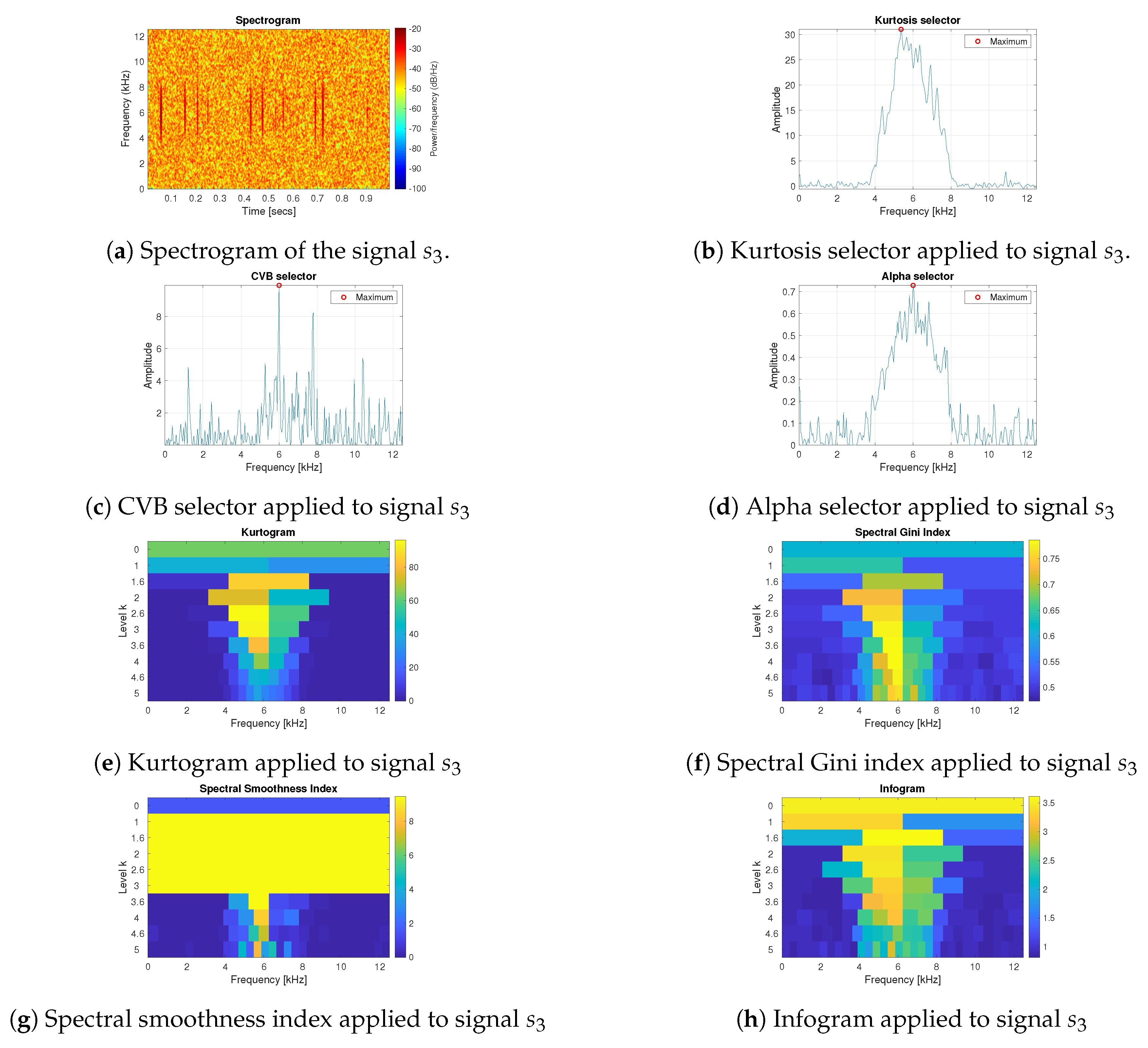
Figure 4 presents the spectrogram and the selectors’ results for the signal with the background of the mixture of Gaussian White Noise and non-cyclic impulses (signal $s_3$) described in Equation (10).

For the non-cyclic impulsive signal $s_3$, all techniques properly select the frequency band where the non-cyclic impulses appear. Note that, none of the methods takes into consideration the cyclic behaviour of the signal, only its impulsiveness. The only exception is the infogram, which takes into consideration both impulsiveness of the signal in the time domain and periodicity in the envelope spectrum; see [48]. However, one can expected it will not point out the frequency band of non-cyclic impulses as there is no periodicity of impulses. In fact, only the SE infogram is sensitive to the impulses. The SES infogram has dispersed values from range 0.45–0.7 kHz, whereas the SE infogram takes values from range 1–6.5 kHz and the maximum value it takes in the middle of this range (6 kHz). However, due to the use of the average of both of them in the infogram definition, see Equation (8), the result is in favor of non-cyclic impulses.

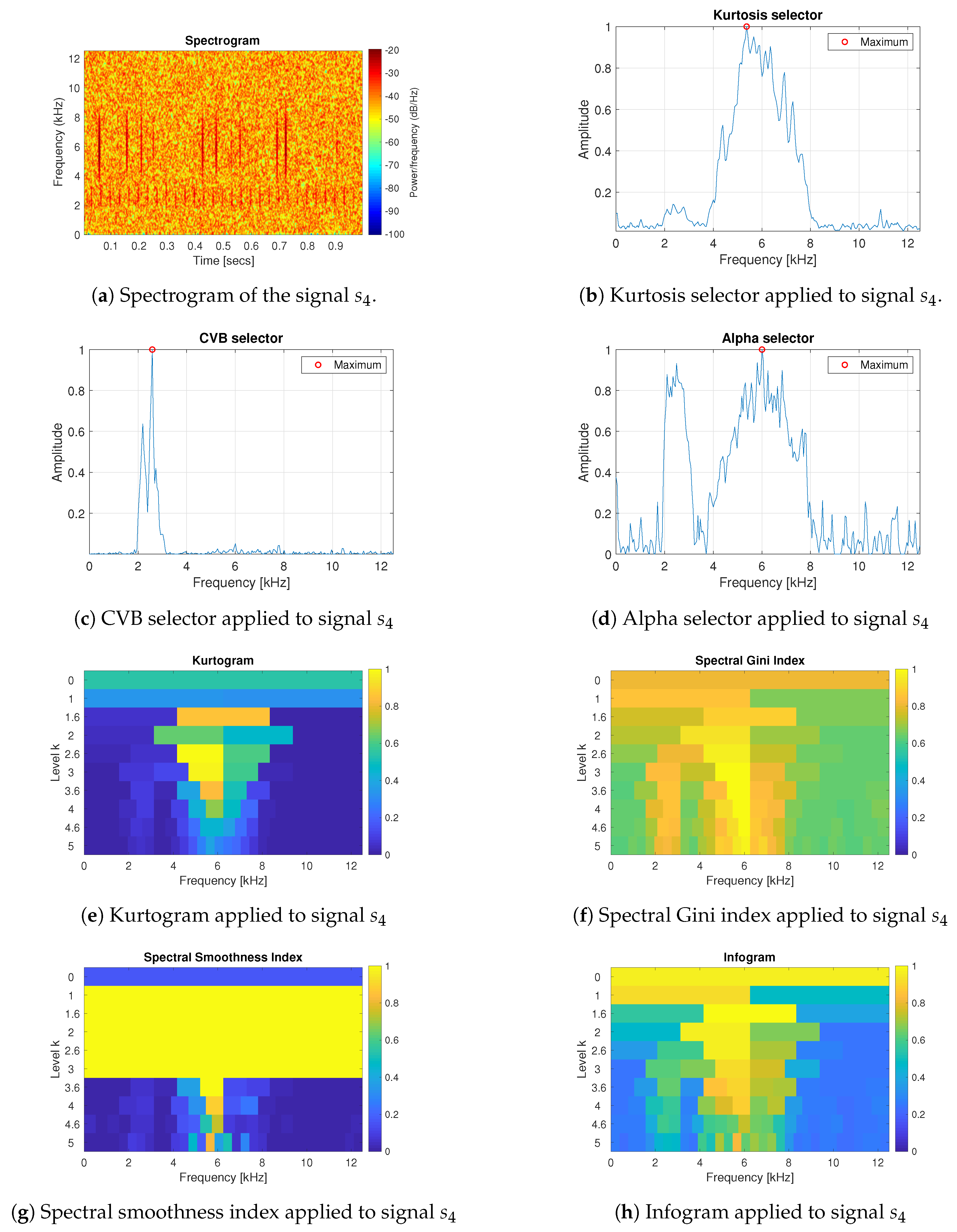
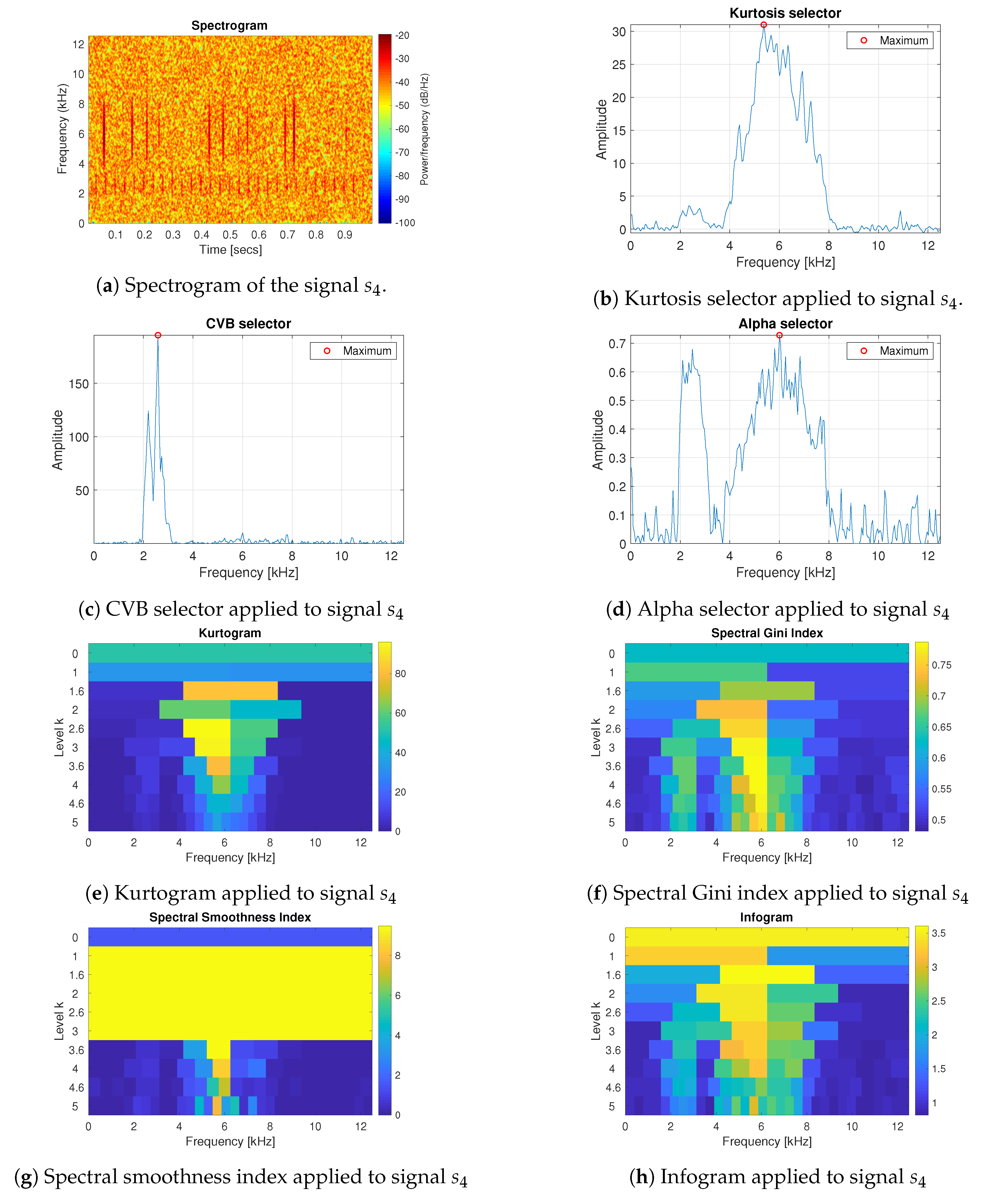
For the most complicated case, presented in Figure 5, i.e., for the signal with a large non-cyclic to cyclic impulses amplitude ratio (signal $s_4$), we expect to find information about the cyclic impulses with possibly suppressed information about non-cyclic impulses. Surprisingly, only the CVB selector correctly identified the frequency band corresponding to the cyclic impulses, based on the distribution of their amplitudes. The Alpha selector, spectral Gini index and infogram indicate both cyclic and non-cylcic impulses frequency ranges. The advantage of the first two ones is that the values of them do not have to be normalized before data filtration, because their values are between 0–1 (according to the definition).

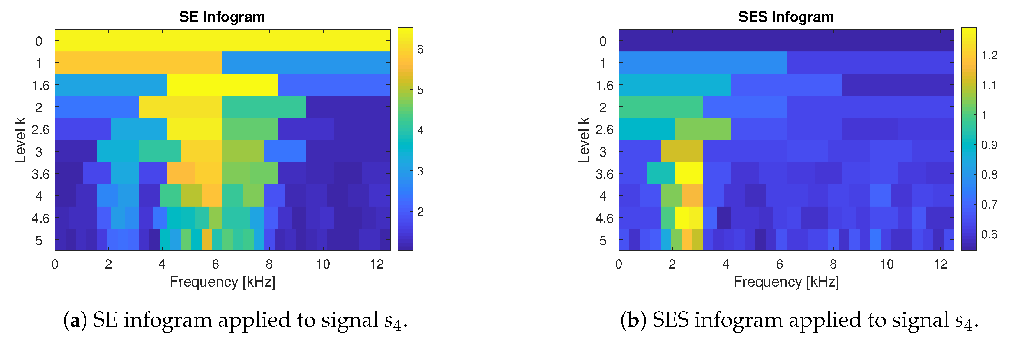
In particular, it is interesting that the Antoni’s infogram method, see [48], which takes into consideration both impulsiveness of the signal in the time domain and periodicity in the envelope spectrum, did not provide clear information for the last type of the signal, i.e., the mixture of the cyclic and non-cyclic impulses (signal $s_4$). As it was mentioned, the infogram is the averaged entropy for a given level of decomposition. In case the cyclic impulses appear in the signal, averaging of high entropy related to high impulses in the time domain, and smaller entropy related to smaller amplitudes of the components in the envelope spectrum, provides some information that favors impulsiveness more than periodicity. We have analyzed separately SE (envelope-based) and SES (spectral envelope-based) parts of the infogram, see Figure 6a,b respectively.

As it was mentioned, for the signal with non-cyclic impulses, the SES infogram contained small values and did not highlight any frequency band. On the other hand, for the mixture of cyclic and non-cyclic impulses, the IFB was correctly recognized but final information was dominated by the SE infogram. It should be mentioned that in [68] the authors suggested the extended version of the infogram with increased accuracy of the IFB selection, i.e., so-called clustered gray infogram. However, there is still place for enhancements and a weighted infogram could be proposed.

Let us note that the normalized version of the selectors’ results (normalization using its maximum value) has been added to the Appendix A to enable the comparison in the same scale. In the main part of the paper, the original scale of the selectors has been proposed in order to obtain the clear information if the given selector properly indicates the informative frequency band.

3.3. Real Data Analysis

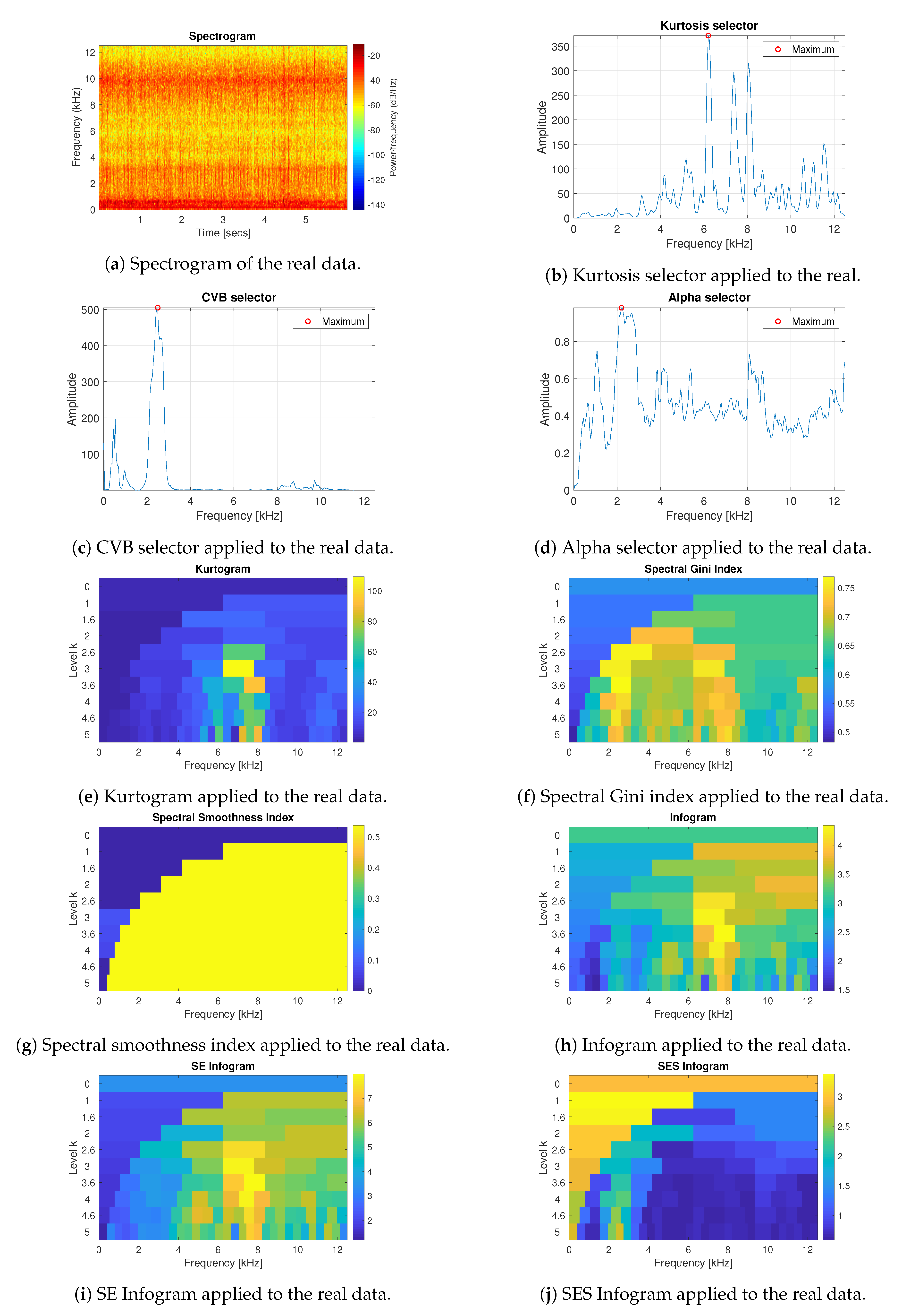
In this section, the tested informative frequency band selectors have been applied to the real vibration data. The effectiveness of the considered methods has been verified on the data origins from the bearing of the crushing machine. However, due to the lack of local fault in the considered vibration data, we decided to introduce an artificial component related to local damage. A similar approach has been performed in [21,42,49]. The signal has been shown in Figure 7. The length of the signal is 6 s and the sampling frequency is 25 kHz. The local fault has been added with the frequency modulation equal to 30 kHz and carrier frequency equal to 2.5 kHz (2–3 kHz). The spectrogram of the data has been presented in Figure 8a. As one can see, the data reveals high-energy wide-band impulses around 0.25, 4.5 and 5.25 s which are related to the falling rocks. The real vibration signal contains various components with a complex structure, and the component related to the damage is almost imperceptible above the noise.

The considered IFB selectors have been applied to the real signal with added fault. The results are presented in Figure 8b–f. Additionally, the results of the SE and SES infograms have been shown in Figure Figure 8g–h. The amplitude of the non-cyclic impulses is smaller than in the considered simulated data but the results of the kurtosis, kurtogram, spectral smoothness index and infogram fail. As it was mentioned in the previous section, the spectral smoothness index is numerically sensitive for small values of the observations. Moreover, the analyzed real signal is 6 times longer than the simulated signals presented in the previous section. Small values and increased signal length cause the selector result to take infinite values. This disadvantage makes it impossible to obtain any sensible result (the infinite values appear up to the 5 level of the decomposition). What is more, the SE infogram does not indicate any impulsiveness in the IFB, only the SES correctly indicates the range of the cyclic impulses occurrence. The Alpha selector and spectral Gini index properly indicate the IFB but with much less selectivity than the CVB selector.

It may happen that the number of random impulses grows up and/or their amplitudes increase. In this case, the spectral distribution of the energy of the analyzed signal will be different and selectivity of the tested selectors could change. Thus, the study of the influence of the number and amplitudes of the non-cyclic impulses on the selectors’ results seems to be interesting.

4. Discussion and Conclusions

In the paper the most prominent techniques of the IFB selection developed in recent years have been tested for benchmark signals that imitate four different cases of the condition of the rotating component of the machine:

• the Gaussian White Noise, which corresponds to the vibration coming from bearings in the healthy condition,
• the Gaussian White Noise with cyclic impulses, which corresponds to the local damaged bearing,
• the non-Gaussian noise, which corresponds to the case without local damage (for the machine is in good condition and executes a specific technological process, e.g., crushing of the rock mass),
• the non-Gaussian noise with cyclic impulses, which corresponds to the damaged bearing in the presence of impulsive noise, associated with the machine operation, e.g., local fault of bearing in the crusher.

In case of the good condition of the machine, we should expect the “flat” distribution of the selector for each technique, whereas for damaged cases one should find some frequency band with a higher value of “diagnostic feature” (selector) than for other frequencies.

In case 1, the values of all considered selectors are relatively small and do not significantly distinguish any frequency band.

For damaged bearing (case 2), all “impulse detectors” point out frequency band where damage-related mechanical impacts excite structural resonance. Unfortunately, there is a high probability that strong impacts related to the technological process will also excite the same structures. Thus, in case of no damage (case 3), one will obtain a suggestion on the informative frequency band that will be a false alarm. Unfortunately, it is a drawback of all tested techniques. To be more precise, the kurtosis selector and kurtogram have 10 times larger values for the frequency band of the non-cyclic impulses than in case of the cyclic impulses of fault. Whereas Alpha selector, spectral Gini index, spectral smoothness index and infogram take similar values in both cases (case 2 and case 3). However, the CVB selector responds more than 17 times more strongly to impulses related to damage than to random impulses related to the operation of the machine. This is related to the definition of the CVB statistic. It omits a significant amount of non-cyclic impulses which fall into the tail of the amplitudes’ distribution.

For the last tested case (case 4), which is the most difficult, there are two types of impulsive (cyclic and non-cyclic) components in the signal. Almost all techniques are focused on the most impulsive component (related to the non-cyclic large observations). The CVB selector, recently proposed in [49] for machine diagnosis, is the unique solution that is based on the relation between amplitude ratio, i.e., the distribution of amplitudes of the background noise, where the predominant noise is Gaussian White Noise and cyclic impulses. Assuming that process-related impulses are much higher than the cyclic impulses, the CVB selector ignore them (they fall into the tail of the distribution) and search for smaller impulses that are cyclic in practice (however, our selector is blind to that property).

In this paper we do not take into consideration the cyclostationary-based approach. However, our future plans are also related to this issue. When large non-cyclic impulses appear in the signal, then the classical cyclostationary methods cannot be applied. Most of them are based on the covariance (or coherence) function. For the impulsive signal, the theoretical covariance does not exist, thus the other measures of dependence need to be applied. Thus, our future plans are related to the application of the alternative measures of dependence to the classical cyclostationary-based methods.

In our diagnostic approach, we always validate the efficiency of SOI extraction by classical envelope analysis. So, for case 3 (no damage), even if all techniques point out some frequency band, it will not be informative in the envelope spectrum (no component with fault frequencies). In case 4, as CVB selects frequencies with cyclic impulses, one may positively recognize the presence of damage.

In this paper we have also checked the results for the real vibration signal. The real data analysis (which corresponds to case 4 of the simulated data) has highlighted several important issues:

• The spectral smoothness index appeared to be numerically sensitive. If the signal is long enough and the values are mostly small in the absolute value then the value of the spectral smoothness index is infinite—this is visible as yellow areas in the map corresponding to the smoothness index.
• Infogram is based on two components, SE and SES. The first one is sensitive for the non-cyclic impulses while the SES indicates the cyclic behaviour of the signal. However, when we take their mean value, then infogram does not give the expected information about the local damage, because the scoring works in favour of non-cyclical impulses. Thus, the results obtained for the real (and simulated) signal indicate that the classical infogram needs to be improved to be more sensitive for the cyclic impulses related to damage than for the non-cyclic ones, which usually have bigger amplitudes. The weighted infogram can be introduced. This is the plan for our future research.
• The kurtosis-based selectors fail as predicted, due to the fact that the kurtosis is very sensitive to outliers, which in the considered cases are the random, non-cyclic impulses with relatively high amplitudes (higher than the cyclic informative impulses). If the amplitudes of impulses are higher, then the value of the kurtosis grows.
• For the presented real data, the amplitude and number of non-cyclical impulses are not very large, thus such selectors as Alpha and CVB selectors, as well as the spectral Gini index, can be successfully used. However, if these values increase (as we have in case 4 for simulated data) then it seems that CVB selector outperforms the other techniques.

As the future work, we also plan to undertake additional study related to the influence of the number and amplitudes of the non-cyclic impulses on the selectors’ results. Currently, this has been done for kurtosis [55] and CVB selector [49]. Such analysis could be interesting for other methods considered in this paper as well.

References

1. Antoni, J.; Randall, R. The spectral kurtosis: Application to the vibratory surveillance and diagnostics of rotating machines. Mech. Syst. Signal Proc. 2006, 20, 308–331. [Google Scholar] [CrossRef]
2. Randall, R.B.; Antoni, J.; Chobsaard, S. The relationship between spectral correlation and envelope analysis in the diagnostics of bearing faults and other cyclostationary machine signals. Mech. Syst. Signal Proc. 2001, 15, 945–962. [Google Scholar] [CrossRef]
3. Barszcz, T.; Jabłoński, A. A novel method for the optimal band selection for vibration signal demodulation and comparison with the Kurtogram. Mech. Syst. Signal Proc. 2011, 25, 431–451. [Google Scholar] [CrossRef]
4. Figlus, T.; Stańczyk, M. A method for detecting damage to rolling bearings in toothed gears of processing lines. Metalurgija 2016, 55, 75–78. [Google Scholar]
5. Yang, Y.; Dong, X.; Peng, Z.; Zhang, W.; Meng, G. Vibration signal analysis using parameterized time–frequency method for features extraction of varying-speed rotary machinery. J. Sound Vib. 2015, 335, 350–366. [Google Scholar] [CrossRef]
6. Abboud, D.; Antoni, J.; Sieg-Zieba, S.; Eltabach, M. Envelope analysis of rotating machine vibrations in variable speed conditions: A comprehensive treatment. Mech. Syst. Signal Proc. 2017, 84, 200–226. [Google Scholar] [CrossRef]
7. Borghesani, P.; Shahriar, M.R. Cyclostationary analysis with logarithmic variance stabilisation. Mech. Syst. Signal Proc. 2016, 70, 51–72. [Google Scholar] [CrossRef]
8. Smith, W.A.; Borghesani, P.; Ni, Q.; Wang, K.; Peng, Z. Optimal demodulation-band selection for envelope-based diagnostics: A comparative study of traditional and novel tools. Mech. Syst. Signal Proc. 2019, 134, 106303. [Google Scholar] [CrossRef]
9. Borghesani, P.; Antoni, J. CS2 analysis in presence of non-Gaussian background noise–Effect on traditional estimators and resilience of log-envelope indicators. Mech. Syst. Signal Proc. 2017, 90, 378–398. [Google Scholar] [CrossRef]
10. Lei, Y.; Lin, J.; He, Z.; Zuo, M.J. A review on empirical mode decomposition in fault diagnosis of rotating machinery. Mech. Syst. Signal Proc. 2013, 35, 108–126. [Google Scholar] [CrossRef]
11. Dybała, J.; Zimroz, R. Rolling bearing diagnosing method based on empirical mode decomposition of machine vibration signal. Appl. Acoust. 2014, 77, 195–203. [Google Scholar] [CrossRef]
12. Peng, Z.; Chu, F. Application of the wavelet transform in machine condition monitoring and fault diagnostics: A review with bibliography. Mech. Syst. Signal Proc. 2004, 18, 199–221. [Google Scholar] [CrossRef]
13. Yan, R.; Gao, R.X.; Chen, X. Wavelets for fault diagnosis of rotary machines: A review with applications. Signal Proc. 2014, 96, 1–15. [Google Scholar] [CrossRef]
14. Figlus, T.; Liščák, Š.; Wilk, A.; Łazarz, B. Condition monitoring of engine timing system by using wavelet packet decomposition of a acoustic signal. J. Mech. Sci. Technol. 2014, 28, 1663–1671. [Google Scholar] [CrossRef]
15. Combet, F.; Gelman, L. Optimal filtering of gear signals for early damage detection based on the spectral kurtosis. Mech. Syst. Signal Proc. 2009, 23, 652–668. [Google Scholar] [CrossRef]
16. Wodecki, J.; Michalak, A.; Zimroz, R. Optimal filter design with progressive genetic algorithm for local damage detection in rolling bearings. Mech. Syst. Signal Proc. 2018, 102, 102–116. [Google Scholar] [CrossRef]
17. Wang, D. Some further thoughts about spectral kurtosis, spectral L2/L1 norm, spectral smoothness index and spectral Gini index for characterizing repetitive transients. Mech. Syst. Signal Proc. 2018, 108, 360–368. [Google Scholar] [CrossRef]
18. Randall, R.B.; Antoni, J. Rolling element bearing diagnostics—A tutorial. Mech. Syst. Signal Proc. 2011, 25, 485–520. [Google Scholar] [CrossRef]
19. Antoni, J. Fast computation of the kurtogram for the detection of transient faults. Mech. Syst. Signal Proc. 2007, 21, 108–124. [Google Scholar] [CrossRef]
20. Obuchowski, J.; Wyłomańska, A.; Zimroz, R. Selection of informative frequency band in local damage detection in rotating machinery. Mech. Syst. Signal Proc. 2014, 48, 138–152. [Google Scholar] [CrossRef]
21. Wodecki, J.; Kruczek, P.; Bartkowiak, A.; Zimroz, R.; Wyłomańska, A. Novel method of informative frequency band selection for vibration signal using Nonnegative Matrix Factorization of spectrogram matrix. Mech. Syst. Signal Proc. 2019, 130, 585–596. [Google Scholar] [CrossRef]
22. Chaari, F.; Leskow, J.; Napolitane, A.; Zimroz, R.; Wylomanska, A. Cyclostationarity: Theory and Methods–IV; Springer: Berlin/Heidelberg, Germany, 2020. [Google Scholar]
23. Lundén, J.; Kassam, S.A.; Koivunen, V. Robust nonparametric cyclic correlation-based spectrum sensing for cognitive radio. IEEE Trans. Signal Proc. 2009, 58, 38–52. [Google Scholar] [CrossRef]
24. Girondin, V.; Pekpe, K.M.; Morel, H.; Cassar, J.P. Bearings fault detection in helicopters using frequency readjustment and cyclostationary analysis. Mech. Syst. Signal Proc. 2013, 38, 499–514. [Google Scholar] [CrossRef] [Green Version]
25. Napolitano, A. Cyclostationarity: New trends and applications. Signal Proc. 2016, 120, 385–408. [Google Scholar] [CrossRef]
26. Antoni, J. Cyclostationarity by examples. Mech. Syst. Signal Proc. 2009, 23, 987–1036. [Google Scholar] [CrossRef]
27. Kruczek, P.; Zimroz, R.; Wyłomańska, A. How to detect the cyclostationarity in heavy-tailed distributed signals. Signal Proc. 2020, 107514. [Google Scholar] [CrossRef]
28. Liu, Y.; Wu, Q.; Zhang, Y.; Gao, J.; Qiu, T. Cyclostationarity-based DOA estimation algorithms for coherent signals in impulsive noise environments. EURASIP J. Wirel. Commun. Netw. 2019, 2019, 81. [Google Scholar] [CrossRef]
29. Gelli, G.; Izzo, L.; Paura, L. Cyclostationarity-based signal detection and source location in non-Gaussian noise. IEEE Trans. Commun. 1996, 44, 368–376. [Google Scholar] [CrossRef]
30. Satija, U.; Mohanty, M.; Ramkumar, B. Cyclostationary features based modulation classification in presence of non Gaussian noise using sparse signal decomposition. Wireless Pers. Commun. 2017, 96, 5723–5741. [Google Scholar] [CrossRef]
31. Liu, Y.; Qiu, T.; Sheng, H. Time-difference-of-arrival estimation algorithms for cyclostationary signals in impulsive noise. Signal Proc. 2012, 92, 2238–2247. [Google Scholar] [CrossRef]
32. Chen, Z.; Yang, Y.; Hu, Z.; Shen, G. Detecting and predicting early faults of complex rotating machinery based on cyclostationary time series model. Vib. Acoust. 2006, 128. [Google Scholar] [CrossRef]
33. Zhao, X.; Qin, Y.; He, C.; Jia, L.; Kou, L. Rolling element bearing fault diagnosis under impulsive noise environment based on cyclic correntropy spectrum. Entropy 2019, 21, 50. [Google Scholar] [CrossRef] [Green Version]
34. Biedka, T.E.; Mili, L.; Reed, J.H. Robust estimation of cyclic correlation in contaminated Gaussian noise. In Conference Record of the Twenty-Ninth Asilomar Conference on Signals, Systems and Computers; IEEE: Piscataway, NJ, USA, 1996; Volume 1, pp. 511–515. [Google Scholar]
35. Ma, X.; Nikias, C.L. Joint estimation of time delay and frequency delay in impulsive noise using fractional lower order statistics. IEEE Trans. Signal Proc. 1996, 44, 2669–2687. [Google Scholar]
36. Yu, G.; Li, C.; Zhang, J. A new statistical modeling and detection method for rolling element bearing faults based on alpha–stable distribution. Mech. Syst. Signal Proc. 2013, 41, 155–175. [Google Scholar] [CrossRef]
37. Katkovnik, V. Robust M-periodogram. IEEE Trans. Signal Proc. 1998, 46, 3104–3109. [Google Scholar] [CrossRef]
38. Jeon, J.H.; Kim, Y.H. Localization of moving periodic impulsive source in a noisy environment. Mech. Syst. Signal Proc. 2008, 22, 753–759. [Google Scholar] [CrossRef]
39. Salehzadeh, N.A.; Ferri, A.M. Vibration-Based Techniques For Damage Detection And Localization In Engineering Structures; World Scientific: Singapore, 2018; Volume 10. [Google Scholar]
40. Liu, R.; Yang, B.; Zio, E.; Chen, X. Artificial intelligence for fault diagnosis of rotating machinery: A review. Mech. Syst. Signal Proc. 2018, 108, 33–47. [Google Scholar] [CrossRef]
41. Zhao, Y.; Li, T.; Zhang, X.; Zhang, C. Artificial intelligence-based fault detection and diagnosis methods for building energy systems: Advantages, challenges and the future. Renew. Sustain. Energy Rev. 2019, 109, 85–101. [Google Scholar] [CrossRef]
42. Wylomanska, A.; Zimroz, R.; Janczura, J.; Obuchowski, J. Impulsive Noise Cancellation Method for Copper Ore Crusher Vibration Signals Enhancement. IEEE Trans. Ind. Electron. 2016, 63, 5612–5621. [Google Scholar] [CrossRef]
43. Wodecki, J.; Michalak, A.; Zimroz, R.; Barszcz, T.; Wyłomańska, A. Impulsive source separation using combination of Nonnegative Matrix Factorization of bi-frequency map, spatial denoising and Monte Carlo simulation. Mech. Syst. Signal Proc. 2019, 127, 89–101. [Google Scholar] [CrossRef]
44. Wyłomańska, A.; Żak, G.; Kruczek, P.; Zimroz, R. Application of tempered stable distribution for selection of optimal frequency band in gearbox local damage detection. Appl. Acoust. 2017, 128, 14–22. [Google Scholar] [CrossRef]
45. Antoni, J. The spectral kurtosis: A useful tool for characterising non-stationary signals. Mech. Syst. Signal Proc. 2006, 20, 282–307. [Google Scholar] [CrossRef]
46. Żak, G.; Wyłomańska, A.; Zimroz, R. Application of alpha-stable distribution approach for local damage detection in rotating machines. J. Vibroeng. 2015, 17, 2987–3002. [Google Scholar]
47. Miao, Y.; Zhao, M.; Lin, J. Improvement of kurtosis-guided-grams via Gini index for bearing fault feature identification. Meas. Sci. Technol. 2017, 28, 125001. [Google Scholar] [CrossRef]
48. Antoni, J. The infogram: Entropic evidence of the signature of repetitive transients. Mech. Syst. Signal Proc. 2016, 74, 73–94. [Google Scholar] [CrossRef]
49. Hebda-Sobkowicz, J.; Zimroz, R.; Pitera, M.; Wylomanska, A. Informative frequency band selection in the presence of non-Gaussian noise—A novel approach based on the conditional variance statistic. Mech. Syst. Signal Proc. 2020. submitted. [Google Scholar]
50. Westfall, P.H. Kurtosis as peakedness, 1905–2014. R.I.P. Am Stat. 2014, 68, 191–195. [Google Scholar] [CrossRef] [Green Version]
51. Joanes, D.; Gill, C. Comparing measures of sample skewness and kurtosis. J. R Stat. Soc. Ser. D Stat. 1998, 47, 183–189. [Google Scholar] [CrossRef]
52. Dyer, D.; Stewart, R. Detection of rolling element bearing damage by statistical vibration analysis. J. Mech. Des. 1978, 100, 229–235. [Google Scholar] [CrossRef]
53. Feng, Z.; Liang, M.; Chu, F. Recent advances in time–frequency analysis methods for machinery fault diagnosis: A review with application examples. Mech. Syst. Signal Proc. 2013, 38, 165–205. [Google Scholar] [CrossRef]
54. Żak, G.; Teuerle, M.; Wyłomańska, A.; Zimroz, R. Measures of dependence for-stable distributed processes and its application to diagnostics of local damage in presence of impulsive noise. Shock Vib. 2017, 2017. [Google Scholar] [CrossRef] [Green Version]
55. Pachaud, C.; Salvetat, R.; Fray, C. Crest factor and kurtosis contributions to identify defects inducing periodical impulsive forces. Mech. Syst. Signal Proc. 1997, 11, 903–916. [Google Scholar] [CrossRef]
56. Samoradnitsky, G. Stable Non-Gaussian Random Processes: Stochastic Models with Infinite Variance; Chapman & Hall: Boca Raton, FL, USA, 1994. [Google Scholar]
57. McCulloch, J.H. Simple consistent estimators of stable distribution parameters. Commun. Stat. Simul. Comput. 1986, 15, 1109–1136. [Google Scholar] [CrossRef]
58. Żak, G.; Wyłomańska, A.; Zimroz, R. Data-driven vibration signal filtering procedure based on the α-stable distribution. J. Vibroeng. 2016, 18. [Google Scholar]
59. Gini, C. Measurement of inequality of incomes. Econ. J. 1921, 31, 124–126. [Google Scholar] [CrossRef]
60. Loza, C.A.; Principe, J.C. Transient model of EEG using Gini Index-based matching pursuit. In 2016 IEEE International Conference on Acoustics, Speech and Signal Processing (ICASSP); IEEE: Piscataway, NJ, USA, 2016; pp. 724–728. [Google Scholar]
61. Wang, Y.; Yang, L.; Xiang, J.; Yang, J.; He, S. A hybrid approach to fault diagnosis of roller bearings under variable speed conditions. Meas. Sci. Technol. 2017, 28, 125104. [Google Scholar] [CrossRef]
62. Hurley, N.; Rickard, S. Comparing measures of sparsity. IEEE Trans. Inf. Theory 2009, 55, 4723–4741. [Google Scholar] [CrossRef] [Green Version]
63. Bozchalooi, I.S.; Liang, M. A smoothness index-guided approach to wavelet parameter selection in signal de-noising and fault detection. J. Sound Vib. 2007, 308, 246–267. [Google Scholar] [CrossRef]
64. Jaworski, P.; Pitera, M. THE 20-60-20 RULE. Discrete Cont. Dyn. Syst. Ser. B 2016, 21. [Google Scholar] [CrossRef] [Green Version]
65. Jelito, D.; Pitera, M. Newfat-tail normality test based on conditional second moments with applications to finance. arXiv 2018, arXiv:1811.05464. [Google Scholar]
66. Brillouin, L. Science and Information Theory; Courier Corporation: Chelmsford, MA, USA, 2013. [Google Scholar]
67. Perthame, B. Boltzmann type schemes for gas dynamics and the entropy property. SIAM J. Num. Anal. 1990, 27, 1405–1421. [Google Scholar] [CrossRef]
68. Li, C.; Cabrera, D.; de Oliveira, J.V.; Sanchez, R.V.; Cerrada, M.; Zurita, G. Extracting repetitive transients for rotating machinery diagnosis using multiscale clustered grey infogram. Mech. Syst. Signal Proc. 2016, 76, 157–173. [Google Scholar] [CrossRef]
Figure 1. Exemplarysimulations of the considered signals: (a) Gaussian White Noise, (b) Gaussian White Noise with the cyclic impulses added, (c) Gaussian White Noise with non-cyclic impulses added, (d) Gaussian White Noise with cyclic and non-cyclic impulses added.
Applsci 10 02657 g001
Figure 2. Results of the informative frequency band selection for 7 different methods for the signal s 1 .
Applsci 10 02657 g002
Figure 3. Results of the informative frequency band selection for 7 different methods for the signal s 2 .
Applsci 10 02657 g003
Figure 4. Results of the informative frequency band selection for 7 different methods for the signal s 3 .
Applsci 10 02657 g004
Figure 5. Results of the informative frequency band selection for 7 different methods for the signal s 4 .
Applsci 10 02657 g005
Figure 6. Results of the informative frequency band selection for signal s 4 SE and Squared Envelope Spectrum (SES) inforgrams.
Applsci 10 02657 g006
Figure 7. Real signal from the crushing machine with the local fault added.
Applsci 10 02657 g007
Figure 8. Results of the informative frequency band selection for 7 different methods for the real data from the bearing of the crushing machine.
Applsci 10 02657 g008