Abstract
Many rural communities in western China use renewable energy-based clean energy supply methods, and the community microgrid system of “photovoltaic + energy storage + electric heating” has been widely used. However, the energy management effect of such a typical rural community microgrid system is not very satisfactory. Aiming at the problem of the comprehensive economic operation of the microgrid system in rural communities, a method for optimizing the operation strategy parameters of typical operating scenarios is proposed, and critical parameters of the real-time energy management strategy of the microgrid system are optimized. Through the evaluation of the annual time-scale simulation results, it is proved that the proposed strategy can improve the comprehensive economic benefits of the operation of the rural community microgrid system (comprehensive economic benefits include electricity bills and energy storage system (ESS) life loss). Relying on the actual community microgrid demonstration project system in western China, a community-level microgrid energy management monitoring system is built. The control strategy proposed in this paper is applied to the demonstration system for experimental verification. The operational data of the demonstration system shows that the proposed method is feasible and effective.
1. Introduction
In recent years, with the rapid development of China’s economy, energy consumption has increased, and traditional energy sources have faced huge challenges. At the same time, the smog problem has attracted increasing attention, and clean energy technologies have been valued. Photovoltaic power generation has undergone many years of development, progressing from centralized to distributed approaches, and is already a relatively mature power generation technology. With the continuous increase of installed capacity of distributed photovoltaic power generation in recent years, photovoltaic power generation has become a large-scale, decentralized feature, and many distributed photovoltaic power generators have been connected to the grid at low voltage. However, further research is required on their safety, stability, reliability, and dissipation. Microgrid systems have become a better solution to the energy supply problem in rural areas [1,2]. With more than one billion people living in rural areas around the world, the issue of energy supply in rural areas needs more attention [3,4]. Nearly 600 million people in China live in rural areas. In order to meet the clean energy supply needs of rural communities in western China, renewable energy-based microgrid systems have been widely used. Combined photovoltaic and energy storage microgrid systems can well solve the problem of clean energy supply in rural communities. At the same time, electric heating is used instead of coal-fired heating to achieve clean heating in rural communities.
Numerous scholars have conducted significant research into energy management of photovoltaic storage microgrid systems. Generally, these systems are divided into two types: grid-connected [5] and off-grid [6]. Reference [7] focused on the PV and storage microgrid system and studied a multi-objective optimal scheduling algorithm that comprehensively considered battery cost and carbon emissions. The algorithm was also applied to microgrids with hybrid renewable generators to solve complex power management problems. Reference [8] investigated the dynamic power optimization control strategy of multiple independent distributed PV and storage systems in microgrids, and applied RTDS simulation to verify the correctness of the theory. The authors of [9] studied the dynamic power optimization strategy of distributed energy storage systems. The distributed energy storage units in the system included EV modules. Reference [10] studied the energy management algorithm of the PV and storage microgrid system based on photovoltaic power generation and load power prediction. The algorithm helped the microgrid system run more stably and reliably.
In the research of rural community microgrids, the literature [11,12] discusses the architecture of rural community microgrid systems in some countries and the specific design methods of these community microgrids. Reference [13] proposed a microgrid energy management system (EMS) to achieve optimal management of isolated rural microgrids. Reference [14] presented the improvement of rural social and economic conditions using microgrid systems to solve the problem of power supply. Reference [15] adopted the DC bus microgrid system to solve the problem of clean energy supply in rural communities. The main goal of the control strategy was to improve the penetration rate of renewable energy in the microgrid system.
In terms of energy management algorithm verification, reference [16] proposed a layered energy management strategy, verified its own algorithm using a laboratory-level experimental platform, and performed a simplified simulation at a given time scale. Reference [17] used a layered multi-agent EMS structure and proposed solutions for improving the calculation speed of energy management. It also utilized a laboratory-level experimental platform to verify its own algorithm. In the actual demonstration project case, the economy of the battery energy storage system (ESS) is an important constraint. Reference [18] fully considered the impact of the energy storage life on the operation strategy. The data in the study came from a real island demonstration project. Most of the research on PV and storage microgrid systems applied in rural communities is at the simulation research stage, and some studies have verified the correctness of their algorithms using a laboratory experimental platform. The rural community PV and storage microgrid system studied in this paper is a real community microgrid demonstration project in northwestern China. The proposed energy management strategy has been implemented in the demonstration system project.
This paper mainly studies the comprehensive economic optimization of rural community microgrid systems, proposes a real-time control strategy considering the cost of the ESS, and adds a priority charging strategy to increase the energy storage life, thereby realizing the real-time optimization control of the community microgrid system. An annual time-scale parameter optimization method based on particle swarm optimization (PSO) is proposed. Two important parameters in the real-time control strategy-the preset energy storage charge value, SOCpro, and the minimum energy storage discharge capacity, SOCmin-are optimized. The objective function comprehensively considers the electricity bill and ESS life loss. Combining the operating characteristics of a typical rural community microgrid system in western China, four types of operating scenarios are summarized, and the optimal setting scheme of operating parameters is studied under these scenarios. The simulation results at the annual time scale prove the correctness of the proposed strategy. This method can adjust the operating parameters to adapt to changes in different seasons and weather to obtain better operating results. The target comprehensively considers the combined impact of energy storage battery life and electricity costs, and economic performance optimization is improved. At the same time, the approach improves the actual application performance of the method. Relying on the demonstration project system of a real community microgrid in western China, a community-level microgrid energy management monitoring system is built, and the multi-scenario variable parameter energy management strategy proposed in this paper is applied to the demonstration system for experimental verification.
2. System Structure
This paper studies a community microgrid demonstration system that includes 24 villas. This community is a typical rural microgrid demonstration system in Qinghai Province, China. An aerial image of the demonstration community is shown in Figure 1. Photovoltaic system installation adopts the form of decentralized installation, taking full advantage of the roof area of the building, forming a small-scale power supply system for self-use and sale of surplus electricity to the utility.

Figure 1.
Aerial image of demonstration community.
The heating method for users in the community is decentralized electric heating, and each villa is designed as a renewable energy-based cogeneration microgrid. In order to improve the power supply reliability of the community microgrid system, the community has set up a centralized ESS. During grid-connected operation, the ESS relies on the time-of-use electricity price policy to improve the economics of the microgrid system; when the utility is out of power, it acts as a backup power source to ensure that the system is continuously powered. The microgrid system structure is shown in Figure 2.

Figure 2.
System structure diagram of the community microgrid.
There are 24 villas in the community, which are powered by renewable energy. The community uses the forms of “photovoltaic + carbon fiber electric heating” and “photovoltaic + air source heat pump” to realize the combined supply of heat and electricity to the main energy users. There are two types of heating load: the carbon fiber geothermal electric heating load, and the air source heat pump heating load. The system consists of the utility, distributed photovoltaic power generation system, battery ESS, and the internal load of the microgrid system. It is a typical “source–utility–load–storage” microgrid system structure. The system is a grid-connected microgrid system, which can realize power exchange with the utility and, as a user, settle electricity charges and distributed generation subsidies with the utility. The grid has a time-of-use electricity price incentive policy for the microgrid systems.
3. Real-Time Control Strategy Considering Cost per kWh of Storage Batteries
3.1. Mathematical Model of Control Strategy
In the grid-connected mode of the distributed microgrid system, the current economically optimal mode is “self-generated self-use, surplus electricity to the utility”. The internal composition of the microgrid can be divided into three categories: resource, load, storage, and distribution grid system. In addition, there are four types of unit: resource, load, storage, and the utility related to the energy flow of the microgrid. If the energy management of the microgrid does not abandon PV power or load controlling under special circumstances, the execution unit is generally the ESS. The main function of the energy storage system is to compensate the energy margin. The mathematical model of the energy margin in the PV and storage microgrid is:
For microgrid systems, this power margin can be compensated by the ESS or the utility:
When choosing which form of electricity to supplement the power margin, the costs of the ESS and the distribution grid system are compared, and the one with the lower use cost is preferred. When the ESS encounters state of charge (SOC) limits or charge and discharge power limits, it is all digested by the distribution grid. The mathematical expressions of the cost per kWh of the ESS and electricity price of the utility are as follows:
where Ces_unit is the cost per kWh of the ESS. This is not the cost of the initial installation of the ESS, but only the cost of battery life loss, because the ESS generally does not need to be replaced except for the batteries. Crep is the total cost of replacing the batteries, Elifecycle is the total energy value that the batteries can emit throughout their life cycle, in kWh, is the charge and discharge efficiency of the ESS, and Cg_unit is the electricity price of the utility.
The implementation of the energy management strategy is mainly achieved by controlling the energy storage power, and the point of common connection (PCC) power can be obtained naturally from the power flow relationship. The execution mathematical expression of the above algorithm is:
In the period when the grid electricity price is relatively high, the ESS is used first. Before controlling the ESS, whether the power in the ESS meets the requirements must be considered.
When the new energy generation in the microgrid exceeds the load power consumption, the corresponding strategies are formulated according to different situations:
(1). The excess photovoltaic power is less than the maximum chargeable power of the ESS:
The ESS absorbs the entire power margin:
(2). The excess power of photovoltaic power generation is greater than the maximum charging power of the ESS, and the distribution grid can absorb excess power:
At this time, the ESS is charged at full power, and the remaining power is absorbed by the distribution grid:
(3). The extra power generated by photovoltaic power generation is greater than the maximum charging power of the ESS and exceeds the dissipation capacity of the distribution grid:
At this time, the ESS is charged at full power, and the distribution grid is fully loaded to send electricity. At the same time, the method of limiting photovoltaic power generation is adopted to maintain system power balance:
where is the power value of photovoltaic power generation abandoned by the microgrid at time t.
There is a possibility in the above situations, that is, the ESS is full:
The ESS cannot be recharged:
For relatively large loads, the power shortage required for the load is supplemented by the utility or ESS. When choosing which electricity to use, it is necessary to compare the electricity price of the utility and the cost per kWh of the ESS; the lower of the two is selected.
When the photovoltaic power generation inside the microgrid is less than the load power consumption, the corresponding strategies formulated according to different situations are as follows.
(1). The electricity price of the utility is lower than the cost of energy storage. The utility can meet the power supply requirements:
Electricity is used from the utility, rather than from the ESS:
(2). The electricity price of the utility is lower than the cost of energy storage. The utility cannot meet the power supply requirements, but adding energy storage can meet the requirements:
The utility is supplied with full power, and the ESS discharges to supplement the remaining margin:
(3). The electricity price of the utility is lower than the cost of energy storage. The utility and energy storage together cannot meet the requirements:
The utility is fully loaded, the ESS is discharged at maximum power, and some unimportant loads are cut out:
(4). The electricity price of the utility is higher than the cost of energy storage. Energy storage can meet the power supply needs:
Energy storage provides the power required by the load:
(5). The electricity price of the utility is higher than the cost of energy storage. Energy storage cannot meet power supply needs, but joining the distribution grid can:
The ESS is discharged at full power, and the remaining power margin is supplemented by the utility:
(6). The electricity price of the utility is higher than the cost of energy storage. The ESS and distribution grid together cannot meet the power supply needs:
Both the energy storage and distribution grid supply power at full load and cut out some unimportant loads:
(7). The battery power is too low, and the utility can supplement the power margin:
The ESS stops working and the power margin is provided by the utility:
(8). The battery power is too low, the utility does not have the ability to supplement the margin:
The energy storage is stopped, the utility is working at full capacity, and some unimportant loads are cut out:
where Pcut(t) is the load power discarded at time t. The program flow chart of the strategy is shown in Figure 3.
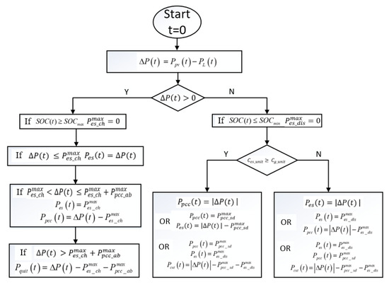
Figure 3.
Energy management strategy program flow chart.
As can be seen from the program flow chart of the energy management strategy, the control strategy first calculates the margin between photovoltaic power generation and load power consumption. There are two types of response according to the difference between supply and demand: when the photovoltaic power generation is larger, the excess power is charged to the battery. After the battery is full, it is sent to the power grid. If the maximum power delivered by the distribution system is reached, a part of the photovoltaic power generation is chosen to be abandoned. When there is relatively little photovoltaic power generation, the strategy will compare the grid electricity price with the cost per kWh of the battery and choose the one with the lower cost to supplement the margin. When the utility and the battery still cannot meet the requirements, some unimportant loads will be cut off.
During long-term simulation of the strategy, it is found that the SOC status of the ESS needs to be improved, especially when the load margin caused by the season is large. Therefore, based on the above strategy, a long-term SOC optimization control method of the ESS is added in which a strategy of charging batteries with preset priority is adopted. The specific implementation scheme is:
- When the SOC status of the ESS is lower than the set value SOCpro, the grid electricity price is lower than the cost per kWh of the ESS, charge the ESS first if possible.
- When the photovoltaic power is greater than the load power, charge the ESS. When the grid price is low, purchase electricity from the distribution grid to ensure the charging power of the ESS.
- When the utility price is low, use as little energy from the batteries as possible, and try to supplement the ESS when SOC is lower than the preset SOCpro.
This strategy can prolong the service life of the ESS and enhance the islanding capability of the microgrid.
3.2. Simulation Results and Analysis
3.2.1. Data and Parameters
The simulation data are historical meteorological data and historical load data of a typical year of the demonstration microgrid system. The data are shown in Figure 4.
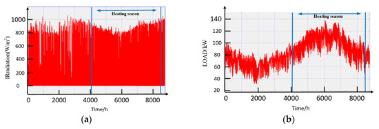
Figure 4.
Simulation data: (a) annual irradiation data; (b) annual load history data.
Figure 4a shows the historical irradiation data of the microgrid system demonstration project location. The abscissa is the hours and the ordinate is the irradiation value. Figure 4b shows the annual load historical data of the demonstration community. The abscissa is time, the unit is hour, and the ordinate is the load power. From the typical annual meteorological data and load data, we can see that the local light resources are very rich, and the maximum annual irradiation can reach 1060 W/m2. The local load varies greatly between seasons and between day and night. The annual maximum load is 138.6 kW, the minimum load is 31 kW, and the average load is 83.78 kW.
The data in the above case are used to verify the energy management algorithm. The simulation parameters are shown in Table 1.

Table 1.
Simulation system parameters.
Time-of-use electricity price parameters are shown in Table 2. After considering the charging and discharging efficiency of the ESS, the actual cost per kWh of the ESS is equivalent to 0.58/0.8 = 0.725 yuan. Therefore, when the electricity price is 0.9402 yuan during peak hours, the electricity price of the utility is higher, so the ESS is preferentially selected to discharge, and the utility is preferentially used in other periods.
Table 2.
Time-of-use electricity price parameters.
3.2.2. Simulation Results and Analysis
The pre-charge optimization strategy for the ESS is not added, and only the maximum and minimum limits of the SOC are added. The annual operation curve of the SOC of the ESS is shown in Figure 5a. The energy storage SOC simulation results after adding the energy storage pre-charge strategy are shown in Figure 5b.
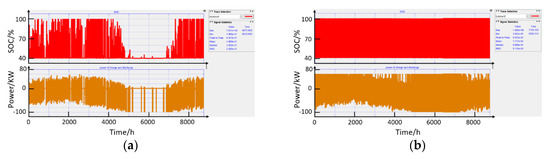
Figure 5.
Simulation results: (a) without pre-charge strategy; (b) with pre-charge strategy.
It can be seen from Figure 5a that the battery has been in a low SOC state for a long time, with an average SOC value of 0.487. It can be seen from Figure 5b that the battery has no long-term power loss, and the average SOC value is 0.772. After the pre-charge strategy is added, the average SOC value of the energy storage battery is improved, and the operating effect of the microgrid system is improved.
3.2.3. Analysis of Economic Benefits
According to the electricity bill settlement method of “self-generated self-use, surplus electricity to the utility” the calculation formula for the total electricity cost of the microgrid system is summarized as:
where COSTt is the total electricity cost; Mg is the electricity fee that needs to be paid for the utility; and Mps is the policy subsidy income for distributed generation. The electricity fee income includes photovoltaic power generation subsidies. The power generation subsidies are 0.37 yuan/kWh and the on-grid tariff is 0.3274 yuan/kWh. Both photovoltaic power generation self-use and grid connection can be subsidized, and grid-connected electricity prices can be directly obtained from grid-connection. Self-use can be reflected in the reduction of grid electricity charges. Because the power of the heating load is large, the overall calculation result of the microgrid still accounts for the payment of the electricity fee to the utility, and the improvement of the operating economy is also reflected in the reduction of the electricity bill.
Calculated according to Equation (48), the comprehensive electricity bill results for the whole year are 52,830 yuan without the charging strategy, and 45,560 yuan after adding the priority charging strategy. These results show that adding the energy storage priority charging strategy has a good optimization effect in terms of battery life and electricity bill.
4. Optimization of Multi-Scenario Parameters Based on PSO
4.1. Parameter Optimization Method Based on PSO
The minimum discharge capacity, SOCmin, is an important parameter associated with battery life. The energy storage charging priority preset value, SOCpro, and the minimum value, SOCmin, of the discharged energy of the ESS are two key parameters that affect the energy storage life and system operation economy. The determination of SOCpro and SOCmin is key to achieving the best operating results.
The simulation of real-time operation strategy was implemented in Simulink. Figure 6 shows the flow chart of the PSO optimization strategy. The PSO randomly generates the initial particles of the SOCpro and SOCmin parameters and inputs the generated parameters into the Simulink simulation model. The Simulink model simulates according to the parameters, calculates performance indicators, and informs the PSO of the results. The particle swarm algorithm judges whether to terminate based on the termination conditions. When the conditions are not met, new particles are updated and continue to be assigned to the simulation model until the parameters with the best running indicators are obtained.
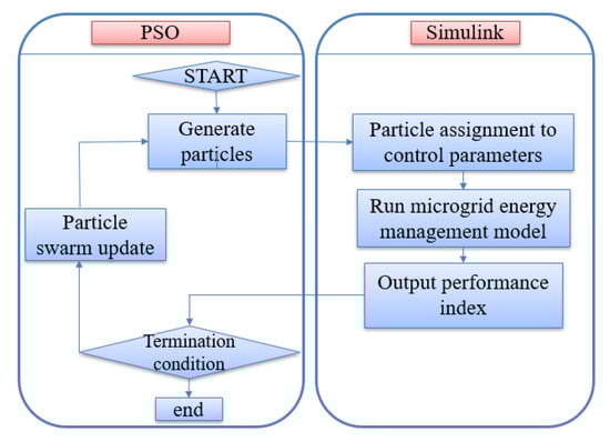
Figure 6.
Particle swarm optimization (PSO) optimization strategy parameter flow chart.
First, we need to establish a mathematical model of the operating battery cost of the energy storage batteries. The commonly used loss cost calculation method is the depreciation method. In an actual PV and storage microgrid system, the depth and rate of charge and discharge are constantly changing. The accuracy of the depreciation method cannot satisfy the needs of practical applications. This article has carried out a quantitative calculation of the loss for a lead–carbon battery system. The loss cost can be accurately expressed by the initial investment of the system and the loss coefficient:
where CBS is the loss cost of the ESS in a specified period, ICBS is the total cost, and DAM is the loss coefficient. The throughput method is used to calculate the life loss coefficient DAM. The throughput of the equivalent total current of the energy storage batteries during the entire life cycle [19] can be used to measure the life loss. The ESS life loss rate can be expressed by the following formula:
where Ac is the equivalent throughput generated in the time period to calculate and Atotal is the equivalent throughput of the entire life cycle.
The approximate calculation formula for the life-cycle throughput of a lead-acid battery is Atotal = 390Q, where Q is the rated ampere-hour of the battery [20]. According to the reference data given by manufacturers, the life of lead–carbon batteries is more than six times longer than that of ordinary lead-acid batteries. It can be roughly obtained that the total throughput of the life cycle of the lead–carbon battery is Atotal = 2340Q.
The calculation of the equivalent throughput, Ac, is related to the actual SOC throughput and the SOC level at runtime. Here, an equivalent conversion coefficient for SOC throughput is introduced. The specific expression is:
where is the equivalent throughput conversion factor and Arc is the throughput of the actual energy storage battery. The calculation formula of the actual throughput is (52). This method calculates both charge and discharge, so the throughput is half of the value:
The determination of is related to the performance of the battery, and needs to be confirmed by referring to the relevant experimental data of the battery. Different SOC states correspond to different throughput conversion coefficients. According to the battery parameters provided by the supplier, the relationship curve between battery SOC and throughput conversion coefficients is shown in Figure 7.
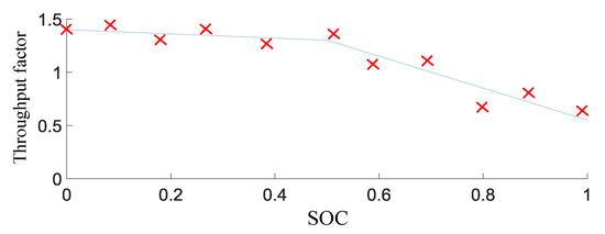
Figure 7.
Relationship curve between and state of charge (SOC).
When the ESS is running, the minimum SOC limit must be set. Above the protection limited SOCmin, and SOC have an approximately linear relationship. is usually obtained by curve fitting. The commonly used expression is:
Considering both the electricity cost formula (Equation (48)) and the ESS life loss formula (Equation (49)), the expression of the comprehensive objective function is:
where α and β are normalization coefficients.
4.2. Multi-Scenario Variable Parameter Optimization
The optimization parameters are implemented by the PSO method. When selecting the optimization parameters, the optimal parameter setting scheme for the annual operation can be obtained by evaluating the comprehensive optimization function. In the process of analyzing the actual demonstration system operating conditions, it was found that the requirements for operating strategies under different weather and load conditions are quite different. The use of uniform parameters throughout the year is not applicable to all scenarios, and may compromise the optimal setting scheme for the whole year. This paper proposes a scenario-based parameter design method. According to the photovoltaic power generation and load characteristics of rural communities in western China, we can summarize four operating scenarios as heating season sunny, heating season cloudy, non-heating season sunny, and non-heating season cloudy. Then, we are able to solve the optimal operating parameters in different scenarios. During the operation, different operating parameters are adopted according to the different scenarios.
Scene 1: Sunny day during the non-heating season
In the non-heating season, the power load is relatively small, and the maximum power of the load is about 55 kW. In sunny conditions, the photovoltaic power generation effect is good, and the maximum power exceeds 100 kW. The ESS is charged at noon when the photovoltaic effect is strong and discharged at night when the load is large. The charging rule is basically one charge and discharge cycle per day. Due to the large photovoltaic power generation, the maximum power of the PCC point power sent to the utility during the day is up to 50 kW, and the load power at night is close to 60 kW. Waveforms of Scene 1 is shown in Figure 8.
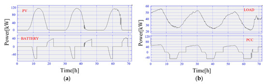
Figure 8.
Waveforms of Scene 1: (a) PV and storage; (b) load and point of common connection (PCC).
The optimal individual fitness value is the lowest value of the comprehensive cost. The total number of iterations is 20. Because the power of photovoltaic power generation is high, its cost value is negative, which means that it can obtain online revenue through photovoltaic power generation. The total comprehensive income obtained in three days is about 232.8 yuan. The simulation waveform is shown in Figure 9.
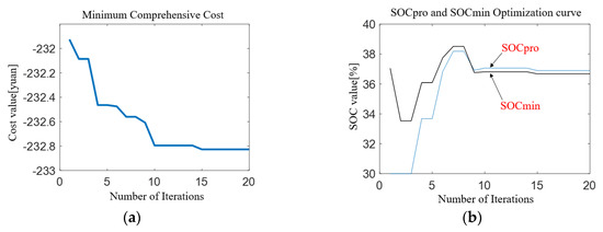
Figure 9.
PSO curves of Scene 1: (a) comprehensive cost; (b) SOCpro and SOCmin.
It can be seen from Figure 9 that the parameter optimization results are SOCpro = 36.5 and SOCmin = 36.4. This means that in the non-heating season, when the photovoltaic power generation is sufficient on sunny days, there is no need to consider the pre-charging of energy storage batteries in advance. Because there is a large amount of photovoltaic power generation on sunny days, the operating strategy will choose to recharge the ESS when photovoltaic power exceeds the load.
Figure 10 shows the simulated waveforms of the SOC curve and the energy storage curve. The implementation effect of the energy storage control strategy is roughly charging during the day and discharging at night. During daytime the ESS can be fully charged, and discharged when the electricity price is high at night; on average, there is one charge and discharge cycle per day.
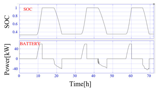
Figure 10.
SOC and storage waveforms of Scene 1.
Scene 2: Cloudy day during the non-heating season
As can be seen in Figure 11, the light intensity is relatively small on cloudy days, and the photovoltaic power generation is low. The maximum power is only about 20 KW. The maximum load power is about 55 KW.
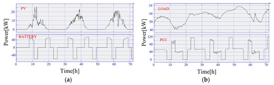
Figure 11.
Waveforms of Scene 2: (a) PV and storage; (b) load and PCC.
The power of the PCC points is all above 0, because the photovoltaic power is small and can be fully self-used, and there is no “remaining power” to sell. Because photovoltaic power generation is always small, it is occasionally necessary to take electricity from the utility to charge the ESS, so the power consumption at the PCC point is often greater than the load power, and the maximum value exceeds 100 kW.
Figure 12 is the optimization curve of SOCpro and SOCmin. The optimization results are SOCpro = 100 and SOCmin = 30.2. The final comprehensive cost result was 1562 yuan. In the scenario where the photovoltaic power generation is very small on cloudy days, attention needs to be paid to charging the ESS in advance. If the ESS is not charged in advance, the photovoltaic power generation is small, so there is no excess electricity to charge the ESS, which will cause the ESS to stay at a low level for a long time and thereby affect the life of the batteries. At the same time, when the electricity price of the utility is high and power needs to be provided for the load, the ESS capacity is insignificant and cannot meet the requirements.

Figure 12.
PSO curves of Scene 2: (a) comprehensive cost; (b) SOCpro and SOCmin.
Figure 13 shows the simulated waveforms of the ESS SOC and charge/discharge power. It can be seen that the ESS is charged during the period when the electricity price is low, and the ESS can be discharged during the two periods when the electricity price is high to provide support for the load electricity consumption.
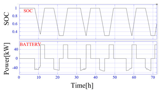
Figure 13.
SOC and storage waveforms of Scene 2.
Scene 3: sunny day during the heating season
In sunny days during the heating season, both the load electricity consumption and photovoltaic power generation are relatively large. The peak power value of photovoltaic power generation during the day reached more than 100 kW, and the peak value of load power consumption at night also reached more than 100 kW.
As can be seen from the power curve of PCC in Figure 14, the span of the micro-grid and utility exchange power is relatively large (much power is generated at day and more is used at night). The maximum power consumption at night reached more than 100 kW, and photovoltaic power generation was sufficient during the day, so the power returned to the grid also reached nearly 50 kW. The total amount of power fluctuations is still relatively large. The large power difference between day and night is a characteristic of sunny days in the heating season.
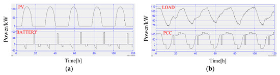
Figure 14.
Waveforms of Scene 3: (a) PV and storage; (b) load and PCC.
As can be seen in Figure 15, the optimization results of the parameter settings are SOCpro = 75.15 and SOCmin = 58.47. If only from the perspective of electricity cost, SOCpro and SOCmin should be set to 30. However, because the algorithm adds consideration of battery life loss, placing it at a lower SOC level has a certain impact on battery life loss. So, through optimization, we found a better solution in this scenario, namely, discharge the electricity when the electricity price is high and the load is heavy, and when the electricity price is relatively low at night, add a certain amount of power to the battery to reduce the influence of lower SOC level on the battery. Charging the battery to 75.15 with the lower electricity price of the grid can keep the battery at a better SOC level while leaving some margin to absorb the photovoltaic power generation the next day. In this way, the optimal result of the comprehensive evaluation cost, considering the loss of the energy storage battery and the power cost, can be obtained as 1459.5 yuan.
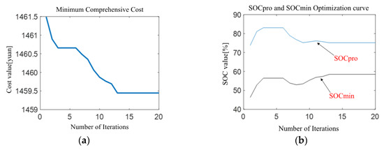
Figure 15.
PSO curves of Scene 3: (a) comprehensive cost; (b) SOCpro and SOCmin.
The SOC and ESS charge and discharge power waveforms are shown in Figure 16. The SOC of the ESS stays around 75 for a period, which is the consequence of charging part of the ESS at night.
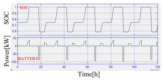
Figure 16.
SOC and storage waves of Scene 3.
Scene 4: cloudy day during the heating season
The demand for the heating season load is relatively large, the minimum value of the load is also above 50 kW, and the maximum value is close to 80 kW. At the same time, the weather is cloudy, photovoltaic power generation is relatively small, and the maximum power generation is only a little more than 30 kW. Waveforms of Scene 4 is shown in Figure 17. Large load demand and insufficient renewable energy supply is the characteristic of this scenario.
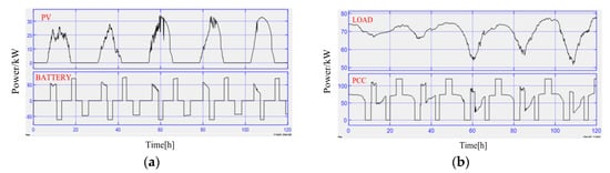
Figure 17.
Waveforms of Scene 4: (a) PV and storage; (b) load and PCC.
Figure 18 shows the simulation curves of PSO optimization. The result is SOCpro = 100, SOCmin = 30, and the minimum value of the comprehensive cost is 2894.
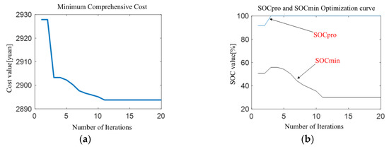
Figure 18.
PSO curves of Scene 4: (a) comprehensive cost; (b) SOCpro and SOCmin.
Due to the large power shortage in this case, we need to pay attention to pre-charging the battery. The load is relatively large, and the photovoltaic power generation is relatively small. It is important to pre-charge the battery.
The SOC and ESS charge/discharge power waveforms are shown in Figure 19. In this case, the power shortage is relatively large. In order to ensure the stability of the power supply of the load, more use of the ESS is needed. Approximately two charge and discharge cycles are required each day to meet the load’s power demand.
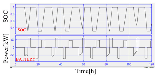
Figure 19.
SOC and storage waveforms of Scene 3.
4.3. One-Year Running Effect Comparison
Through the evaluation of the annual operation effect, according to the same optimization design method, optimal parameters for the annual comprehensive operation can be obtained: SOCpro = 100, SOCmin = 40. After setting the parameters of SOCpro and SOCmin, the annual operation of the microgrid system is simulated, and the annual operation curve regardless of the scenario can be obtained as shown in Figure 20.
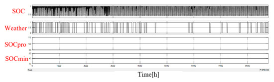
Figure 20.
Simulation waveforms of constant parameters.
The waveforms in Figure 20 from top to bottom are: SOC, weather parameters, SOCpro, and SOCmin. Figure 21 shows the results of the simulation of the comprehensive cost.
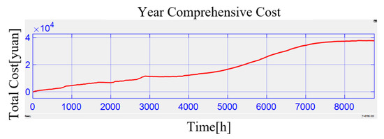
Figure 21.
Comprehensive cost value of constant parameters.
In Figure 21, the ordinate is the comprehensive cost value and the abscissa is the simulation time. The final comprehensive cost simulation result is 37,754 yuan.
According to the four scenarios discussed in the previous section, four sets of optimal parameters can be obtained, as shown in Table 3.
Table 3.
Optimal parameter values in different scenarios.
According to the annual historical irradiation curve and historical weather conditions, the annual weather conditions curve can be plotted, as shown in Figure 22, where 1 represents sunny and 0 represents cloudy.
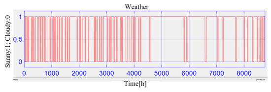
Figure 22.
Statistics of weather conditions.
According to different weather conditions and seasons, different parameters are set for different scenarios, and the running curve is shown in Figure 23.
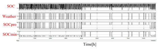
Figure 23.
Variable parameter simulation waveform.
As can be seen from the above figure, the weather parameters constantly change. According to local heating policies, the heating time is from October 15 to April 15 of the following year, and the corresponding simulation hours are 4020 h to 8400 h. The two parameters of SOCpro and SOCmin constantly change with the weather and season to adjust the operating strategy of the microgrid system to achieve better operating results. The final comprehensive cost operation results are shown in Figure 24, with a comprehensive cost value of 36,187 yuan.
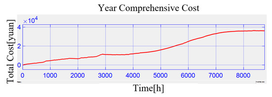
Figure 24.
Comprehensive cost value of variable parameters.
It can be seen from Table 4 that the multi-scenario variable parameter optimization method proposed in this paper has better performance of power grid electricity costs and battery loss costs.
Table 4.
Annual operation effect of different strategies.
After using variable parameter operation, the annual comprehensive operating cost is reduced by 1567 yuan compared with the overall optimized constant parameter operation strategy, for a cost saving rate of 4.15%. The operating cost is also 3945 yuan lower than the basic real-time control strategy, for a cost saving rate of 9.76%. The use of different operating strategy parameters according to different scenarios is worth adopting in an actual demonstration system.
5. Introduction and Analysis of Experimental Results of the Demonstration System
5.1. Introduction of the Demonstration System
The structure of the demonstration community microgrid system is shown in Figure 2. The entire community includes a typical community microgrid system, a public building sub-microgrid system, a family sub-microgrid system, a rooftop photovoltaic installation capacity of 100 kW, a container-type 100 kW/210 kWh battery ESS, and three sets of 5 kWh distributed lithium battery ESS; the total load in the community is about 130 kW. Photographs of key equipment in the microgrid system are shown in Figure 25, including rooftop photovoltaics, energy storage batteries, electric heating facilities, air-source heat pumps, and monitoring systems.
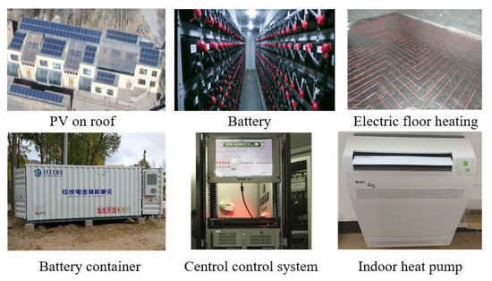
Figure 25.
Photos of key equipment of the microgrid.
The microgrid monitoring system interface is shown in Figure 26. The monitoring system realizes the monitoring and control of photovoltaic power, the ESS, the load, and other equipment in the community microgrid system. The monitoring system can display the status of photovoltaic power generation and the status of energy storage batteries. It can monitor the real-time data of load power consumption and the weather data. For controllable equipment, the monitoring system can send instructions to control it. The monitoring system includes a local database function to record and store operating data. Historical data can be displayed in the form of curves, lists, and so on. The strategy of energy management is realized by programming in the monitoring system.
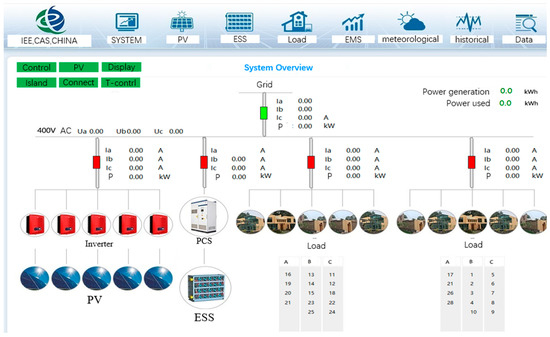
Figure 26.
Interface of the monitoring system.
5.2. Analysis of Running Effect and Experimental Waveform
Figure 27, Figure 28, Figure 29 and Figure 30 display the history curves of the monitoring system. In each figure, the abscissa is time and the ordinate is power. The red curve is the photovoltaic power curve, referred to as PV; the green curve is the ESS power curve, referred to as ESS; positive values represent ESS charging and negative values represent ESS discharge; purple curves are load power curves, referred to as LOAD; and the blue curve is the PCC power curve, referred to as PCC. A positive signifies that the microgrid system uses power from the grid, and a negative sign represents that the microgrid system sends power to the grid. The right side is a graphic illustration that shows the maximum and minimum values of the corresponding data.
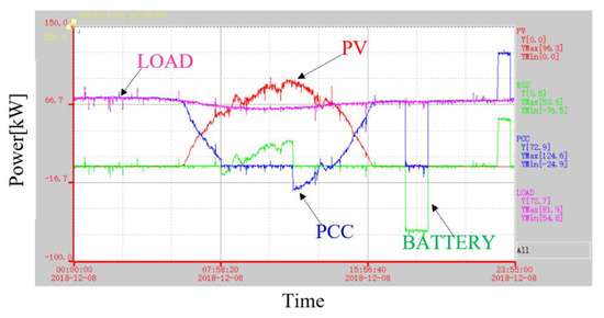
Figure 27.
Experimental waveform of a sunny day in the heating season.
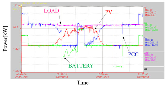
Figure 28.
Experimental waveform of a cloudy day in the heating season.
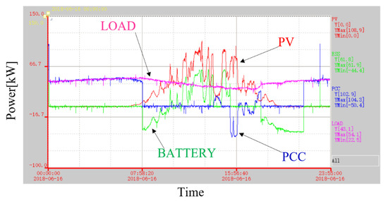
Figure 29.
Experimental waveform of a sunny day in the non-heating season.
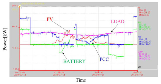
Figure 30.
Experimental waveform of a cloudy day in the non-heating season.
From the experimental waveforms, it can be seen that when the photovoltaic power generation is greater than the load power after 8 am, photovoltaic power generation charges the ESS. After 12:00, the ESS is full, and excess electricity from photovoltaic power generation is sold to the grid. At night when the electricity price is very high, the ESS releases electricity to make up for the shortage of load. In order to prevent the battery from stagnating at a low level for a long period of time, resulting in excessive life loss, the battery is charged until the power level reaches the SOCpro value during the night when the electricity price is low.
It can be seen from the actual running waveform that because of the program for pre-charging the battery, the ESS is charged from the grid when the midnight electricity price is low. When the electricity price is high at 8 a.m., photovoltaic power generation cannot meet the load demand, the ESS is discharged, and the power shortage is replenished. After the early peak electricity price, the electricity price in the afternoon is in the parity period, and the electricity price of the grid is lower than the cost of the ESS. During the period when the peak electricity price is high at night, the power in the ESS is discharged. Then, electricity is replenished at low electricity prices during the night.
This scenario does not include pre-charging of the ESS because, during the day, photovoltaic power generation is greater than the load, and there is therefore a lot of electricity. Basically, the battery can be fully charged during the day, and will not be in a low SOC level for a long time, which will damage the battery life. From the waveforms of the demonstration system operation, it can be seen that at night, there is no operation of charging the ESS. At around 8 a.m. when the peak electricity price is high, photovoltaic power generation cannot yet meet the load power consumption, and the ESS discharge makes up for the margin. After 9 a.m., the photovoltaic power generation exceeds the load power consumption, and the ESS begins to charge. Because the ESS is not charged at night, the ESS is fully charged until 4 p.m., and the remaining portion of photovoltaic power generation is sold to the grid. During the night when the electricity price is high, the ESS discharges to supplement the power margin.
In this scenario, photovoltaic power generation is relatively small and, at the same time, the power of the load will be less than the heating season. Because photovoltaic power experiences greater power changes due to weather, it can basically be used by the load. In order to prevent the ESS from being in a low-power state for a long period of time, a control strategy that preferentially charges ESS is implemented. From the waveform of the demonstration operation, it can be seen that the ESS is charged from the utility at the moment when the night electricity price is low. At the time when the early peak electricity price is high, photovoltaic power generation cannot meet the load power consumption, and the ESS discharges to supplement the power shortage. In the afternoon, the ESS is charged at the parity time of the utility. First, it is charged with photovoltaic power, then the shortage is supplemented by the utility. The ESS will be discharged during the period when the peak electricity price is high, late at night, to supply power for the load.
6. Conclusions
The cost of ESS is relatively high at this stage. When microgrid operation economics are optimized, the impact of ESS life loss needs to be considered. This paper establishes an operation control strategy model of a rural community PV and storage microgrid system and proposes an economic optimized operation strategy suitable for the “self-generated self-use, surplus electricity to the utility” mode. The strategy considers the influence of the cost per kWh of the energy storage battery and adds a long-term operating ESS pre-charge strategy. The operating strategy uses different control strategies to control the ESS at different times of the time-of-use electricity price to achieve economic optimization under real-time operation.
This paper focuses on the setting of two important parameters, SOCpro and SOCmin, and proposes a parameter optimization method using PSO. The objective function considers two factors: the electricity cost and the ESS life loss. The calculation of electricity costs considers factors such as time-of-use electricity prices, subsidies for distributed photovoltaic power generation, load electricity consumption, and other factors. The ESS life loss is calculated using the equivalent throughput method, and the impact of low battery static electricity on life loss is added.
Combined with the actual operation of the rural community microgrid in western China, four typical operating scenarios are summarized, namely, sunny in the heating season, cloudy in the heating season, sunny in the non-heating season, and cloudy in the non-heating season. Parameter optimization was performed for four typical scenarios to obtain the optimal parameters in different scenarios. Comparing the annual time scale operation effect of the variable parameter strategy and the constant parameter strategy, the results show that the variable parameter strategy can reduce the overall cost by 4.15%, which is worth adopting.
Relying on the 100-kilowatt-level engineering demonstration system, a community-level microgrid energy management monitoring system is built, and the control strategy proposed in this paper and the multi-scenario parameter optimization system obtained through simulation are experimentally verified. The experimental results of four typical operational scenarios are introduced, and the operation data of the demonstration system show that the proposed method is feasible and effective.
Author Contributions
Conceptualization and methodology, L.G.; validation, L.G. and Z.Y.; writing, L.G.; supervision, H.X.; project administration, Z.Y.; funding acquisition, Y.W. All authors have read and agreed to the published version of the manuscript.
Funding
This research was funded by [the Qinghai Major Science and Technology program] grant number [2019-GX-A] and [the K.C. Wong Education Foundation] grant number [GJTD-2018-05].
Conflicts of Interest
The authors declare no conflict of interest.
Nomenclature
| Symbol | Description |
| Ppv(t) | Photovoltaic power at time t |
| PL(t) | Load power at time t |
| The power margin | |
| Pes(t) | Power of energy storage system |
| Ppcc(t) | Power of PCC point |
| Ces_unit | Cost per kWh of the ESS |
| Crep | Total cost of replacing the batteries |
| Elifecycle | Total energy of the ESS |
| Cg_unit | Utility electricity price |
| V(t) | The utility electricity price at time t |
| Charge and discharge efficiency of the ESS | |
| The maximum chargeable power of the ESS | |
| Maximum dischargeable power of the ESS | |
| Maximum absorbable power of the PCC | |
| Maximum power the PCC point can provide | |
| The abandoned power of PV | |
| SOC(t) | The SOC of ESS at time t |
| SOCmax | Maximum SOC limit |
| SOCmin | Minimum SOC limit |
| Pcut(t) | The cut power of unimportant load |
| COSTt | Total electricity cost |
| Mg | Electricity fee for the utility |
| Mps | Policy subsidy income for distributed generation |
| CBS | The loss cost of the ESS |
| ICBS | Total cost of the ESS |
| DAM | Loss coefficient of the ESS |
| Ac | Equivalent throughput in the time period to be calculated |
| Atotal | Equivalent throughput of the entire life cycle |
| Equivalent throughput conversion factor | |
| Comprehensive cost |
References
- Hatziargyriou, N. Microgrids: Architecture and Control; Wiley-IEEE Press: Piscataway, NJ, USA, 2013. [Google Scholar]
- Mohn, T. It Takes a Village: Rural Electrification in East Africa. IEEE Power Energy Mag. 2013, 11, 46–51. [Google Scholar] [CrossRef]
- Maheshwari, Z.; Ramakumar, R. Smart Integrated Renewable Energy Systems (SIRES) for rural communities. In Proceedings of the 2016 IEEE Power and Energy Society General Meeting (PESGM), Boston, MA, USA, 17–21 July 2016. [Google Scholar]
- Anvari-Moghaddam, A.; Monsef, H.; Rahimi-Kian, A. Cost-effective and comfort-aware residential energy management under different pricing schemes and weather conditions. Energy Build. 2015, 86, 782–793. [Google Scholar] [CrossRef]
- Carpinelli, G.; Mottola, F.; Proto, D.; Russo, A. A Multi-Objective Approach for Microgrid Scheduling. IEEE Trans. Smart Grid 2017, 8, 2109–2118. [Google Scholar] [CrossRef]
- Mercier, P.; Cherkaoui, R.; Oudalov, A. Optimizing a Battery Energy Storage System for Frequency Control Application in an Isolated Power System. IEEE Trans. Power Syst. 2009, 24, 1469–1477. [Google Scholar] [CrossRef]
- Wu, X.; Cao, W.; Wang, D.; Ding, M. A Multi-Objective Optimization Dispatch Method for Microgrid Energy Management Considering the Power Loss of Converters. Energies 2019, 12, 2160. [Google Scholar] [CrossRef]
- Morstyn, T.; Hredzak, B.; Agelidis, V.G. Network Topology Independent Multi-Agent Dynamic Optimal Power Flow for Microgrids with Distributed Energy Storage Systems. IEEE Trans. Smart Grid 2016, 9, 3419–3429. [Google Scholar] [CrossRef]
- Wang, T.; O’Neill, D.; Kamath, H. Dynamic Control and Optimization of Distributed Energy Resources in a Microgrid. IEEE Trans. Smart Grid 2015, 6, 2884–2894. [Google Scholar] [CrossRef]
- Michaelson, D.; Mahmood, H.; Jiang, J. A Predictive Energy Management System Using Pre-Emptive Load Shedding for Islanded Photovoltaic Microgrids. IEEE Trans. Ind. Electron. 2017, 64, 5440–5448. [Google Scholar] [CrossRef]
- Martin-Martínez, F.; Sánchez-Miralles, A.; Rivier, M. A literature review of Microgrids: A functional layer-based classification. Renew. Sustain. Energy Rev. 2016, 62, 1133–1153. [Google Scholar] [CrossRef]
- Shahzad, M.K.; Zahid, A.; Ur Rashid, T.; Rehan, M.A.; Ali, M.; Ahmad, M. Techno-economic feasibility analysis of a solar-biomass off grid system for the electrification of remote rural areas in Pakistan using HOMER software. Renew. Energy 2017, 106, 264–273. [Google Scholar] [CrossRef]
- Kumar, A.; Deng, Y.; He, X.; Kumar, P.; Bansal, R.C. Energy management system controller for a rural microgrid. J. Eng. 2017, 13, 834–839. [Google Scholar] [CrossRef]
- Jha, S.K.; Stoa, P.; Uhlen, K. Socio-economic Impact of a Rural Microgrid. In Proceedings of the 4th International Conference on the Development in the in Renewable Energy Technology (ICDRET), Dhaka, Bangladesh, 7–9 January 2016. [Google Scholar]
- Gunasekaran, M.; Mohamed Ismail, H.; Chokkalingam, B.; Mihet-Popa, L.; Padmanaban, S. Energy Management Strategy for Rural Communities’ DC Micro Grid Power System Structure with Maximum Penetration of Renewable Energy Sources. Appl. Sci. 2018, 8, 585. [Google Scholar] [CrossRef]
- Luna, A.; Meng, L.; Diaz Aldana, N. Online Energy Management Systems for Microgrids: Experimental Validation and Assessment Framework. IEEE Trans. Power Electron. 2017, 33, 2201–2215. [Google Scholar] [CrossRef]
- Harmouch, F.Z.; Ebrahim, A.F.; Esfahani, M.M.; Krami, N.; Hmina, N.; Mohammed, O.A. An Optimal Energy Management System for Real-Time Operation of Multiagent-Based Microgrids Using a T-Cell Algorithm. Energies 2019, 12, 3004. [Google Scholar] [CrossRef]
- Zhao, B.; Zhang, X.; Chen, J. Operation optimization of standalone microgrids considering lifetime characteristics of battery energy storage system. IEEE Trans. Sustain. Energy 2013, 4, 934–943. [Google Scholar]
- Sauer, D.U.; Wenzl, H. Comparison of different approaches for lifetime prediction of electrochemical systems—Using lead-acid batteries as example. Power Sources 2008, 176, 534–546. [Google Scholar] [CrossRef]
- Jenkins, D.P.; Fletcher, J.; Kane, D. Lifetime prediction and sizing of lead-acid batteries for microgeneration storage applications. IET Renew. Power Gener. 2008, 2, 191–200. [Google Scholar] [CrossRef]


© 2020 by the authors. Licensee MDPI, Basel, Switzerland. This article is an open access article distributed under the terms and conditions of the Creative Commons Attribution (CC BY) license (http://creativecommons.org/licenses/by/4.0/).