An ADS-Based Sparse Optimization Method for Sonar Imaging Sensor Arrays

Abstract

The Mills Cross sonar sensor array, achieved by the virtual element technology, is one way to build a low-complexity and low-cost imaging system while not decreasing the imaging quality. This type of sensor array is widely investigated and applied in sensor imaging. However, the Mills Cross array still holds some redundancy in sensor spatial sampling, and it means that this sensor array may be further thinned. For this reason, the Almost Different Sets (ADS) method is proposed to further thin the Mills Cross array. First, the original Mills Cross array is divided into several transversal linear arrays and one longitudinal linear array. Secondly, the Peak Side Lobe Level (PSLL) of each virtual linear array is estimated in advance. After the ADS parameters are matched according to the thinned ratio of the expectant array, all linear arrays are thinned in order. In the end, the element locations in the thinned linear array are used to determine which elements are kept or discarded from the original Mills array. Simulations demonstrate that the ADS method can be used to thin the Mills array and to further decrease the complexity of the imaging system while retaining beam performance.

1. Introduction

Sonar imaging is widely used for underwater detection applications, such as military defense, engineering maintenance, accident rescue, topographic survey, and so on [1]. A variety of array sensor systems play an important role in sonar imaging. The conventional underwater array imaging systems generally include two main forms: front-view or side-scan sonar imaging. Both imaging approaches employ a one-dimensional (1D) linear array sensor to obtain two-dimensional (2D) imaging, and then further to get three-dimensional (3D) imaging [2]. Recently, a sonar imaging approach with a 2D array sensor has been in use, which adopts a subarray system and implements a multibeam technique. However, the imaging quality based on the subarray system is related to the number of subarrays and array elements. The higher the imaging quality, the more subarrays and array elements are required. This results in a very complex imaging system and increased manufacturing cost. One of the ways to solve this contradiction is to use sparse array sensor and synthetic aperture imaging technology. The first task is to design a sparse layout of array sensor elements while maintaining beam performance and imaging quality [3].

The sparse layout optimization of the sonar array sensor resembles that of a radar array antenna. Therefore, sparse methods for the sonar array sensor can be developed from the sparse radar array antenna [4]. These methods are mainly divided into two categories: random and determined. For the random methods, the distribution characteristics of beam response can be utilized in sparse optimization. Yan Tao employed an improved genetic algorithm (GA) to obtain 2D sparse planar arrays, in which he established an optimization model with the goal of minimizing the peak side lobe level (PSLL). This method not only provides a specific sparse ratio of the array elements, but also maintains the array performance [5]. Rodríguez used the simulated annealing algorithm (SAA) to synchronously optimize the locations and the weighting coefficients of linear array elements when the side lobe of the beam pattern meets the relevant requirements [6]. The Convex Optimization (CO) method proposed by D’Urso can globally optimize the positions and weighting coefficients of the array elements to obtain the maximal thinned array, and effectively reduce the computational complexity and PSLL values [7]. For a rectangular array with unequal amplitude excitation, Yuan Zhihao employed the improved Particle Swarm Optimization (PSO) algorithm to perform sparse optimization of the array, in which the inertia weighting strategy is utilized for the global optimal particle perturbation and hopping. The improved algorithm greatly improves the convergence speed and accuracy [8]. The random array optimization algorithms are implemented repeatedly in the iterative search strategy to achieve one global optimal solution under constrained conditions. However, the common disadvantage of the random methods is the huge computational workload and the lack of real-time capacity in practical applications.

Liu Xuesong proposed a low-complexity cross-type array, in which the multifrequency (MF) emission and parallel subarray (PS) beam-forming algorithms are used. The obtained sparse array can greatly bring down the hardware cost and complexity of the imaging system [9]. This scenario uses the Cyclic Difference Set (CDS) to perform sparse optimization on Multiple Inputs and Multiple Outputs (MIMO) arrays. The CDS method can obtain the prior estimates of PSLL and the position of array elements. However, this method cannot provide a solution to those arrays with an arbitrary aperture size due to the binary property of the autocorrelation function of the CDS [10]. Dong Jian adopted the Almost Difference Set (ADS) to perform sparse optimization of MIMO uniform linear arrays. The ADS method can determine the position of each array element of the transmit array and receive array, and perform a prior estimation on the side-lobe level of the beam pattern. Therefore, the ADS method greatly enhances the service efficiency of the array element and can be popularized for large arrays [11]. Because deterministic algorithms do not require iteration or fewer iteration times, the solution speed is faster and the convergence is better. Therefore, the ADS method may have great potential in the sparse optimization of the array sensor. Luo Yi-yang constructed a nonequidistant sparse antenna array on the Latin square array structure by using the cyclic difference set as the unit. This method can ensure high sparsity with low lateral radiation [12]. Matteo Carlin analyzed the robustness of the analytical refinement algorithm based on the Almost Difference Set when there are defective elements in the linear array, and derived the PSLL statistics of the damage layout from the values of different aperture sizes [13].

The ADS method possesses many advantages, such as obtaining a prior estimation on the side-lobe level of the array beam power pattern, enhancing the using efficiency of array element, fitting the large size array, and avoiding the binary property of the autocorrelation function. Therefore, the ADS method is suggested to further thin the Mills Cross array sensor, which is based on virtual array element technology in this paper. The purpose is to further reduce the number of array elements, the manufacturing cost, and the system complexity when using the cross array sensor while maintaining beam pattern and imaging quality.

2. Almost Difference Set and Sparse Optimization of Mills Cross Array

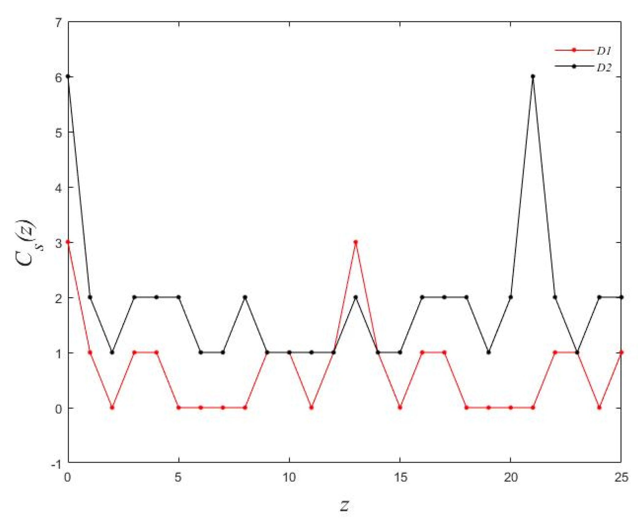
2.1. Almost Difference Sets

Let D be a K subset of an Abelian group G of order N, and the differences between any two nonzero elements in D will form a set F. If t nonzero elements in G appear in each of Λ times, and the remaining (N-t-1) nonzero elements appear (Λ + 1) times each, then D is said to be (N, K, Λ, t)-ADS [14,15].

If the set D is (N, K, Λ, t)-ADS, and there is a binary sequence of length N that satisfies D, where the n-th element is represented as:

$$a_n=\{\begin{array}{c}1,n\in D\\ 0,\mathrm{other}\end{array}$$

(1)

Then, the characteristic binary sequence (that corresponding to D) $S=\left\{s_n,n\in Z\right\}$ is expressed as:

$$s_n=\{\begin{array}{l}1,{\mathrm{mod}}_N\left(n\right)\in D\\ 0,\mathrm{other}\end{array}$$

(2)

where, ${\mathrm{mod}}_N(n)$ means taking the modulus of N, and there exists a periodic autocorrelation function $C_s\left(z\right)$ about $S_n$:

$$C_s\left(z\right)={\displaystyle \sum _{n=0}^{N-1}{S}_n{S}_{n+z}},\mathrm{z}\in \mathbb{Z}$$

(3)

The autocorrelation function is characterized as ‘‘three-valued’’:

$$C_s(\mathrm{z})=\{\begin{array}{ll}K,& \mathrm{z}=0\\ \Lambda +1,& z\in L\\ \Lambda ,& \mathrm{other}\end{array},K\ge \Lambda +1$$

(4)

In the period $z\in \left[0,N-1\right]$, L being a set of $N-1-t$ elements (i.e., L = {$l_p\in \mathbb{Z}$; $p=1,...,N-1-t$ }). For illustrative purposes, let us consider the examples of ADSs reported in

Table 1. All Peak Side Lobe Levels (PSLLs) for the arrays thinned by ADS.

K	Sparse Ratio	$\mathit{E}\left\{{\mathsf{\Phi }}_{\mathit{N}}^{\mathbf{min}}\right\}$	$\mathit{P}\mathit{S}{\mathit{L}}_{\mathbf{min}}^{\mathit{o}\mathit{p}\mathit{t}}\left(\mathbf{dB}\right)$	$\mathit{P}\mathit{S}{\mathit{L}}_{\mathbf{max}}^{\mathit{o}\mathit{p}\mathit{t}}\left(\mathbf{dB}\right)$
20	50%	2.65	−13.5	−7.57

of the literature [16] together with the corresponding binary sequences and autocorrelation functions. In the interest of saving space, however, only two ADS sequences D₁ and D₂ are given. They are {5, 6, 9} and {0, 1, 3, 13, 16, 17}, respectively. The autocorrelation functions $C_s^{\mathrm{ADS}}\left(z\right)$ of D1 and D2 are shown in Figure 1.

Through the comparison and analysis, we can see that the autocorrelation function $C_s^{\mathrm{ADS}}\left(z\right)$ of a (N, K, Λ, t)-ADS is close to that of the (if any) corresponding (N, K, Λ)-CDS.

$$C_s^{\mathrm{CDS}}\left(z\right)=\{\begin{array}{l}Kz=0\\ \Lambda \mathrm{other}\end{array}$$

(5)

In addition, the ADSs share several other properties with the CDSs; for example, both ADS and ADS cannot be defined for every value of N, K, Λ and t. However, it should be noted that the autocorrelation function of CDS is “binarity”. As a result, the condition limitations of ADS are fewer than those of CDS. Therefore, ADS is able to generate more sets and arrays, and thus it is easier to obtain the array form achieving the designed beam pattern [16].

$$K\left(K+1\right)=t\Lambda \left(N-1-t\right)(\Lambda +1)$$

(6)

Another characteristic of ADS is cyclic shift, assuming that $D^{(\sigma )}$ is a sequence obtained by cyclic shifting $\sigma$ of the original ADS sequence. These shifted ADS sequences are called the isomorphic ADS sequences and have the same parameters as the original ADS sequences (N, K, Λ, t). Since the maximum number of cyclic shifts $\sigma$ is the length N of the original ADS sequence, N different isomorphic ADS sequences can be obtained by cyclic shift, which are expressed as:

$$D^{(\sigma )}=\{d_k^{(\sigma )}={\mathrm{mod}}_N(d_k+\sigma ),k=1,...,K\}$$

(7)

Here, $\sigma \in \mathbb{Z}$.

2.2. ADS-Based Arrays

According to the investigations from Oliveri [17], ADS can be used to thin the linear array sensors. The basic idea is to arrange N array elements into a one-dimensional linear array and express them according to the ADS sequence, and then the power function and PSLL estimation are obtained by the autocorrelation function of the linear array and its “ternary value” characteristics. Through the power function and the isomorphism ADS sequences, the discarded or reserved elements in the original linear array are determined. This will ensure that the thinned array sensor achieves or approximates the required beam performance.

Suppose that the weighting coefficient $w\left(n\right)$ is used to indicate whether the array element exists, here $w(n)\in \{0,1\},n=1,...,N$. When $w\left(n\right)$ is equal to 1 and 0, respectively, the reservation or desertion of the array element are indicated. The array factor can be expressed as:

$$S\left(u\right)={\displaystyle \sum _{n=0}^{N-1}w\left(n\right)\exp \left(i2\pi n\gamma u\right)}$$

(8)

where $\gamma$ is the ratio of the array element spacing to the signal wavelength, $u=\sin \theta$, and $\theta$ represents the angle between the signal and the normal direction. In addition, the weighting coefficients of the ADS array by can be obtained according to Equations (1) and (2):

$$w\left(n\right)=\{\begin{array}{l}1,n\in D\\ 0,\mathrm{other}\end{array}$$

(9)

From Equation (8), when the sampling interval $u=1/N\gamma$, the beam power pattern ${\left|S\left(u\right)\right|}^2$ at $u=k/N\gamma$ is expressed as:

$${\left|S\left(k/N\gamma \right)\right|}^2=\Xi \left(k\right),k=0,1,...,N-1$$

(10)

According to the ADS autocorrelation function, the beam power pattern $S\left(u\right)$ at $u=k/N\gamma$, that is, the sampling of $S(u)$, is the Fourier transform of the autocorrelation function $C_s(z)$ [17]:

$$\Xi \left(k\right)=\triangleq {\displaystyle \sum _{z=0}^{N-1}{C}_s\left(z\right)}\exp \left(i2\pi zk/N\right)$$

(11)

It is further expressed as:

$$\Xi \left(k\right)=K-\Lambda +N\Lambda \delta \left(k\right)+\psi \left(k\right)$$

(12)

For Equation (12), $\delta \left(k\right)$ is the discrete impulse function [$\delta \left(k\right)=1$ if $k=0$, and $\delta \left(k\right)=0$ otherwise], $\Psi \left(k\right)\triangleq IDFT\left\{\psi \left(z\right)\right\}$ where $\psi \left(z\right)\triangleq {\displaystyle {\sum }_{p=1}^{N-1-t}\delta \left(z-z^r\right)}$ and $z^r$, $r=1,...,N-1-t$ are the indexes at which $C_s\left(z\right)=\Lambda +1$ (an analogous relationship holds true in the linear case [17]). According to Equation (4), the ADS sequence exhibits a three-level autocorrelation function. The PSLL of the beam power direction satisfies the inequation [18]:

$$PSL{L}_{MIN}^{opt}\le PSL{L}_{DW}^{opt}\le PSL{L}_{}^{opt}\left\{D\right\}\le PSL{L}_{UP}^{opt}\le PSL{L}_{MAX}^{opt}$$

(13)

where $PSL{L}^{opt}={\min }_{\sigma \in [0,N-1]}\left\{PSLL\left(D^{\left(\sigma \right)}\right)\right\}$, $PSL{L}_{DW}^{opt}=\max \left\{PSL{L}^{\infty },PSL{L}^{\min }\right\}$, $PSL{L}_{UP}^{opt}=E\left\{{\Phi }_N^{\min }\right\}PSL{L}^{\infty }$, $PSL{L}_{MIN}^{opt}=PSL{L}_{MIN}^{\infty }$ and $PSL{L}_{MAX}^{opt}=E\left\{{\Phi }_N^{\min }\right\}PSL{L}_{MAX}^{\infty }$, being $E\left\{{\Phi }_N^{\min }\right\}\approx 0.8488+1.128{\log }_{10}N$ [18] and $PSL{L}^{\min }=E\left\{{\Phi }_N^{\min }\right\}{\min }_n\left(P{P}_{\infty ,n}\right)/P{P}_{\infty ,0}$. It should be pointed out that $PSL{L}_{DW}^{opt}$ and $PSL{L}_{UP}^{opt}$ are determined when the ADS sequence is available since they require the knowledge of the coefficients $P{P}_{\infty ,n}$. On the contrary, $PSL{L}_{MIN}^{opt}$ and $PSL{L}_{MAX}^{opt}$ can be always computed a priori from Equations (14) and (15).

$$PSL{L}_{MIN}^{opt}=\frac{K-\Lambda -1+\sqrt{t(N-t)/(N-1)}}{(N-1)\Lambda +k-1+N-t}$$

(14)

$$PSL{L}_{MAX}^{opt}=E\left\{{\Phi }_N^{\min }\right\}\frac{K-\Lambda -1+\sqrt{t\left(N-t\right)}}{\left(N-1\right)\Lambda +k-1+N-t}$$

(15)

According to the relevant theory and research of ADS, it is extremely difficult to deduce a more accurate $PSL{L}_{DW}^{opt}$ and $PSL{L}_{DW}^{opt}$ as the limits of PSLL estimation completely from mathematics, while it is relatively easy to use $PSL{L}_{DW}^{opt}$ and $PSL{L}_{UP}^{opt}$, and it can meet the requirements of PSLL prior estimation of the beam power pattern [18]. For illustrative purposes, let us use the cases in the literature [16]. When using the (42, 21, 10, 31)-ADS sequence, the ADS-based MIMO transmitting array is $D_{21}^{\left(0\right)}$ = (0, 1, 2, 4, 7, 8, 11, 12, 13, 14, 16, 17, 20, 22, 25, 27, 35, 36, 37, 38, 39) and 41 other isomorphic sequences are obtained by applying cyclic shifting to the original ADS. Then, calculate the PSLLs of different ADS-based virtual arrays to obtain the optimal PSLL.

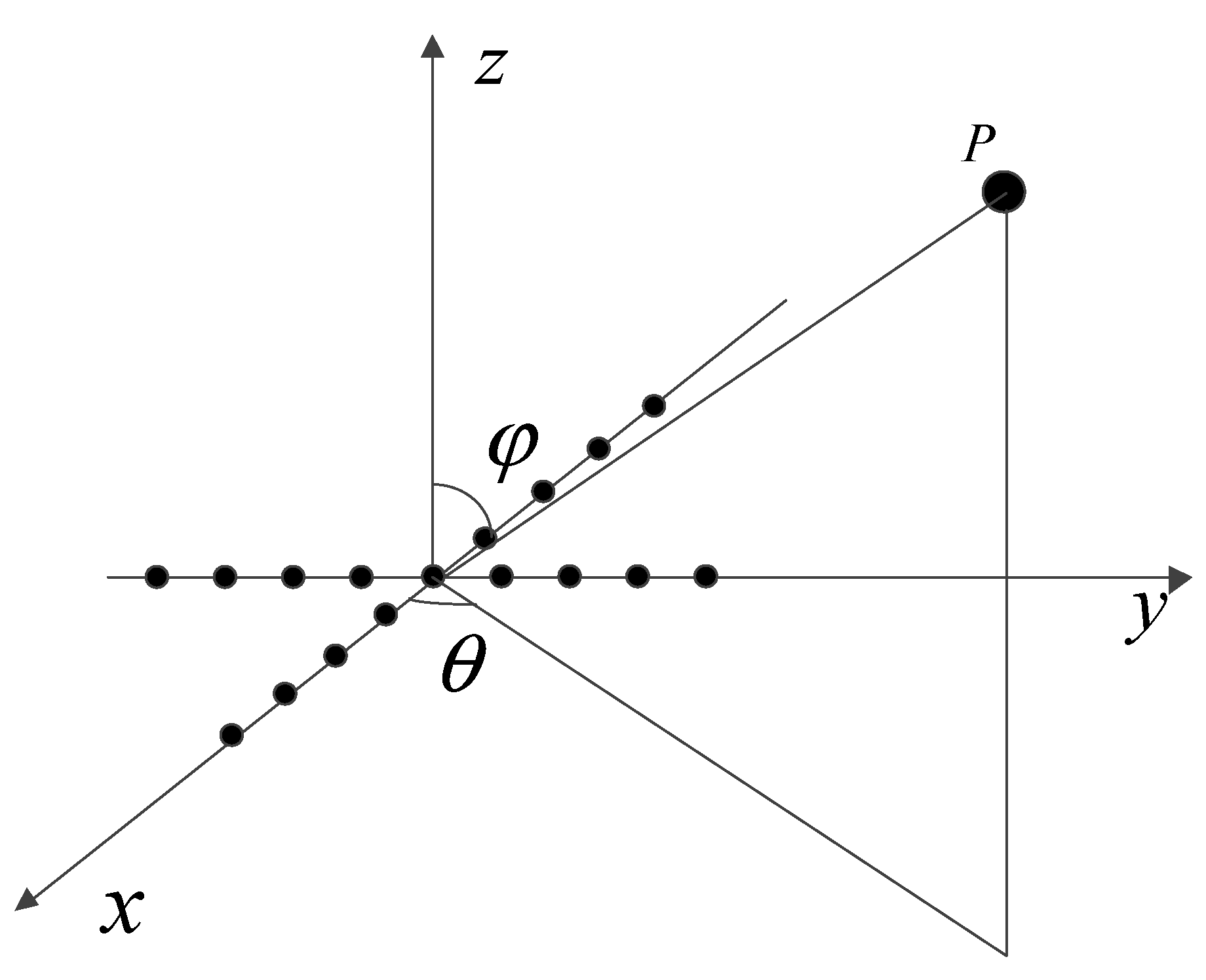
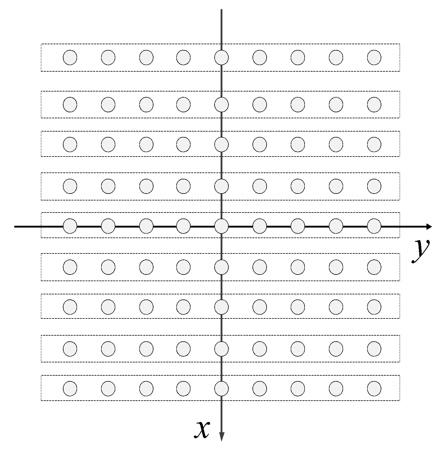
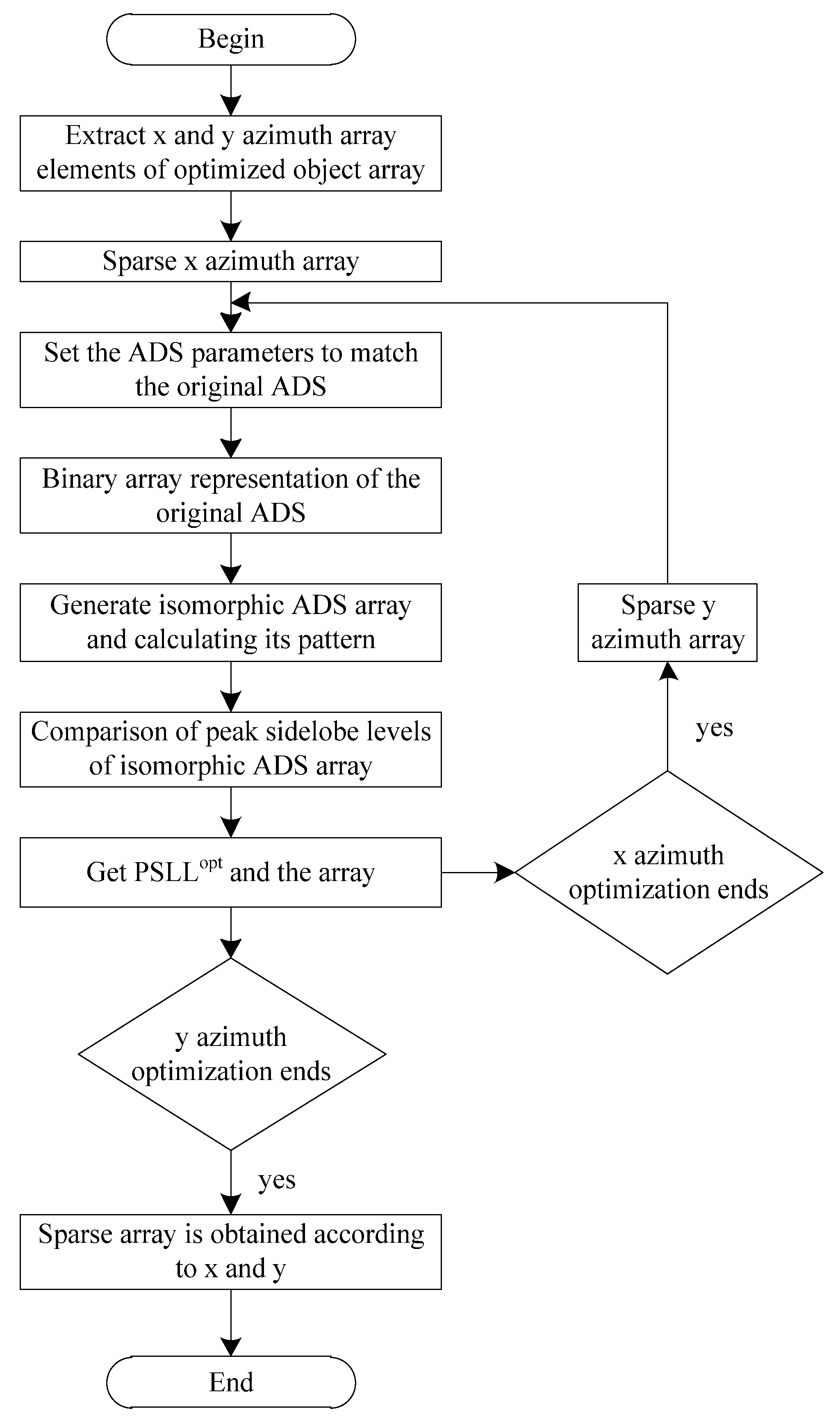
3. Mills Cross Array Optimization Using ADS Method

The Mills Cross array sensor is a kind of regular array, which is obtained by virtual array element technology. It has been widely investigated in radar and sonar imaging [19]. Figure 2 shows a Mills Cross array with nine transmit and nine receive elements, which form a transmit and receive array, respectively, arranged on the X and Y axes of the Cartesian coordinate system. According to the equivalent phase principle, the Mills Cross array can determine a 9 × 9 virtual array sensor under the condition of far field, as shown in Figure 3. Therefore, this will allow to greatly decrease the complexity of the imaging system compared with the common real array. However, there is still some degree of redundancy in the Mills Cross array sensor when the number of array elements reaches a certain scale.

Because the Mills Cross array sensor is one two-dimensional planar array, there will be a problem of large computational complexity if the existing ADS optimization strategies are directly used [20]. For this reason, this paper proposes a different optimization strategy to avoid this problem. Firstly, the two-dimensional virtual array sensor from the Mills Cross array should be divided into several virtual linear arrays with equal length. As shown in Figure 3, the virtual circle represents the locations of virtual array elements, and each dashed frame is one virtual linear array of the same length. According to array theory [21], each virtual linear array can be regarded as a “virtual large array element”. In this way, in the direction perpendicular to the virtual linear array, a linear array composed of virtual linear array can be formed. According to the expected beam pattern and the estimated PSLL, the linear array can be thinned by the ADS method to choose a virtual linear array, and then some virtual array elements are gained in the same way. As such, the sparse optimization of two-dimensional virtual array sensors can be realized from the azimuth X and Y. Finally, the position of these resultant sensors is used for reverse calculation to reserve and discard the array elements in the original Mills Cross array. As a result, a two-dimensional array with a more sparse and nonuniform “cross” shape is obtained. The optimization implementation is described in Figure 4.

Because the beam performance of the array is greatest when the sensors are spaced at half the wavelength of the transmitting sound wave [21], the virtual array elements from the Mills Cross array are also on the grid at half wavelength. Secondly, after the finite length linear array from the virtual array elements is thinned by the ADS method, the sensor arrangement of the sparse array is represented by a binary sequence, that is, 1 is represented as array element retention and 0 as array element abandonment. The obtained K array elements are sparsely distributed at N half-wave positions. Moreover, the advantages of the ADS method are shown by the low redundancy of fewer array elements. In this paper, 40 transmitting and 40 receiving elements were used in the original Mills Cross array.

Because the thinned ratio in ADS research is usually 50%, that is, K is 20, the parameters (N,K,Λ,t) in the ADS library are only (40, 20, 9, 10), and the corresponding original sequence is:

$$D_{20}^{\left(0\right)}=\left(1,3,4,5,7,8,11,14,16,17,18,19,22,24,25,26,27,31,32,36\right)$$

The PSLL range of the corresponding array expressed by this sequence is shown in Table 1.

After the Mills Cross array with 40 transmitting elements and 40 receiving elements is further thinned by the (N, K, Λ, t)-ADS method, the element locations in the thinned array are determined, as shown in Figure 5a. The two-dimensional virtual array formed from the thinned array is shown in Figure 5b. The vacant position on the grid in Figure 5 is a discarded array element.

4. Analysis of ADS Thinned Array

4.1. Effect of Cycle Index

According to the PSLL estimation inequality of the beam pattern in the ADS method, the PSLL bounds of transmitting and receiving arrays can be obtained for the original Mills Cross array. Based on the equivalent relation of product theorem, the beam pattern of virtual array can be expressed as:

$$P_{virtual}(\theta ,\phi )=P_t(\theta ,\phi )\cdot P_r(\theta ,\phi )$$

(16)

where $P_{virtual}(\theta ,\phi )$, $P_t(\theta ,\phi )$, and $P_r(\theta ,\phi )$ represent the normalized power pattern of the virtual array, the transmitting array, and the receiving array, respectively.$(\theta ,\phi )$ indicates the angle of the beam. For the normalized beam power pattern of the transmitting or receiving array, the maximum PSLL is 1 (main lobe region or grid lobe), which satisfies the virtual array power pattern:

$$PSL{L}_r^{\min }\le PSL{L}_{virtual}^{\min }\le PSL{L}_{virtual}^{\max }\le PSL{L}_r^{\max }$$

(17)

Because the obtained virtual array also satisfies the prior PSLL prediction of the ADS linear array, the prediction PSLL inequality of the transmitting and receiving array can be used. Figure 6 is a power cross-sectional view of an obtained array beam pattern in the x direction when $\theta =0$, $\phi =0$ and the number of cycles is 0, 15, and 28, respectively (in order to make the curve clear, only the beam patterns of three isomorphic sequences are given, because the different array element layout have different power patterns, including the optimal one). It can be seen from Figure 6 that the beam performance of the array sensor is different with different cycles. When $\sigma =28$, the PSLL of the array power pattern is the lowest. Therefore, in order to obtain a sparse array with the optimal PSLL, the number of cycles needs to be correct. In Figure 6, PSLL-max and PSLL-min are the estimated maximum and minimum PSLL, respectively.

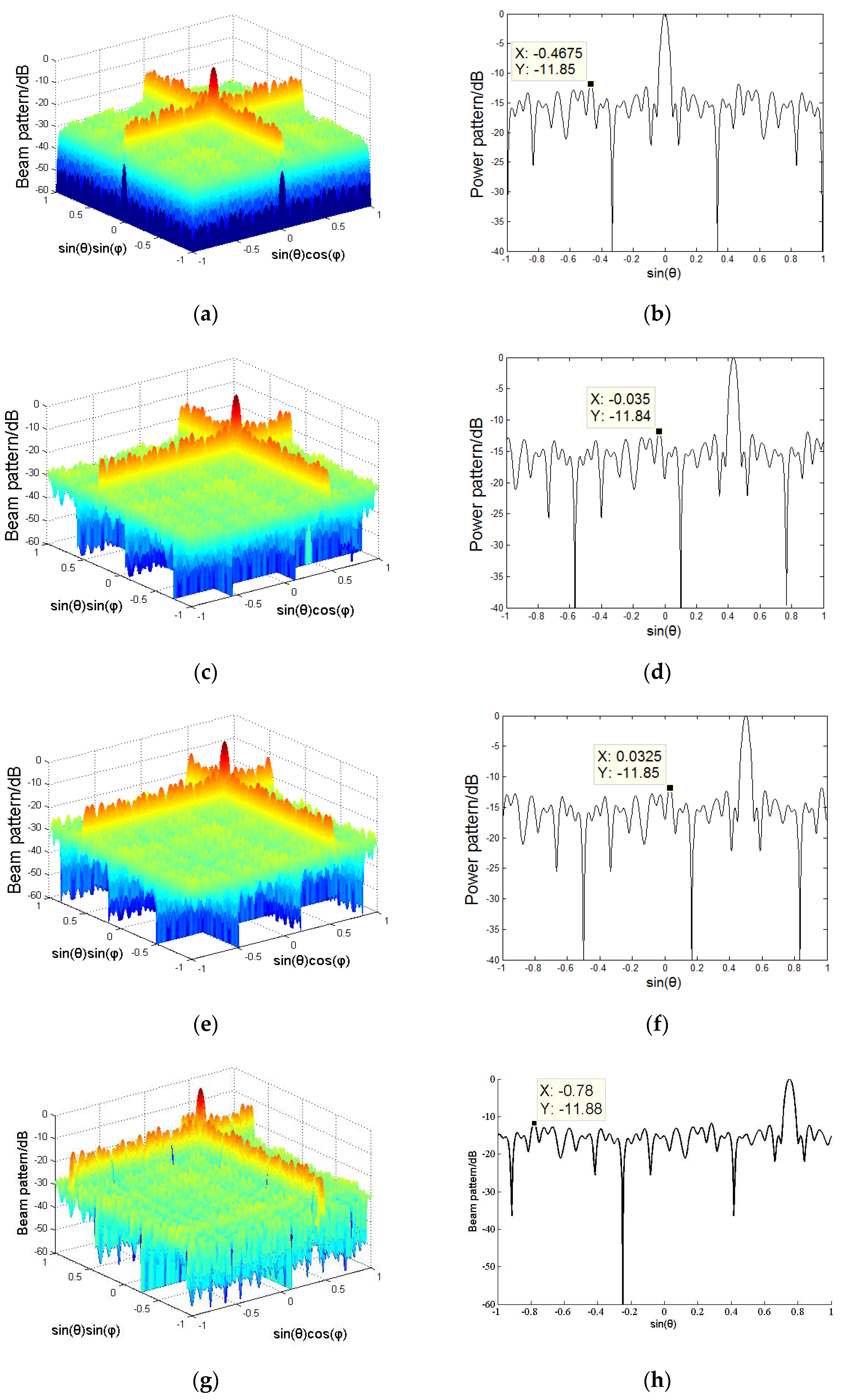
4.2. Azimuth Angle Performance

In order to evaluate the beam performance of the obtained array in different directions, the 3D power patterns were simulated in different directions. In this paper, the beam power diagrams are given in Figure 7 when $\theta$ and $\phi$ are 0°, 30°, 45°, 60°, and 75°, respectively. The main lobe width is about 2.6° in the case of −3 dB, and increases slightly as the azimuth angle increases. The slight change of the main lobe width is probably a result of the size of the array aperture being small when compared to the detection range, only about 30 cm under a carrier frequency of 100 KHz. In addition, the amplitude of the main lobe remains consistent when the azimuth angle is less than 45° and drops significantly when the azimuth angle exceeds 45°. Nevertheless, the PSLL also remains relatively steady from 11.83 to 11.85 when the azimuth angle changes. It can also be seen from these simulation results that the width and amplitude of the main lobe and the PSLL change slightly within the scope of azimuth angular variation.

In order to further identify the performance of the array thinned by ADS, we compare the beam pattern of the target array with those of the original Mills Cross array with 40 × 40 elements and the sparse array by the CDS method. When using the CDS method, the parameters (N, K, Λ) are set as (40, 21, 1) to make the element count of the thinned array approximately the same as that after ADS. The PSLL values of the beam patterns at various steering angles are given in

Table 2. PSLL values of the beam patterns for three arrays at various steering angles.

	Steering Angle	0°	30°	45°	60°	75°
Array
Original Mills		−13.27	−13.27	−13.26	−13.22	−13.25
Thinned by CDS		−12.33	−12.35	−12.32	−12.12	−12.07
Thinned by ADS		−11.85	−11.84	−11.85	−11.88	−11.83

. Meanwhile, the beam pattern graphs of the Mills Cross array and the thinned array by CDS are also presented here. The beam patterns are given in the case of $\theta$ and $\phi$ at 45° and are shown in Figure 8 and Figure 9.

These results indicate that the original Mills array has the best beam performance compared to the other thinned arrays with roughly equal beam width. The major difference is the PSLL values of the beam patterns. This difference is due to a larger thinned ratio in CDS and ADS sequence results in the spatial undersampling of the array. Comparison of the two arrays thinned by CDS and ADS demonstrates this point. In our investigation, the thinned ratios of the CDS and ADS methods are 21 and 20, respectively, and the element counts of the two virtual arrays are 441 and 400, respectively. Therefore, the PSLL values of the beam patterns following CDS method are slightly lower than those using ADS. In addition, ADS is able to generate more sequence sets and arrays compared to CDS, and thus it is easier to obtain an estimated array. Unfortunately, we cannot deduce other sets due to our weaker mathematical ability, but we will contact Oliver’s research group and invite them to guide us in creating a new set. At that time, we will provide the further investigation results. Here, the results are just to demonstrate that the ADS method can be applied to sparse the sensor array.

4.3. Azimuth Resolution

In this paper, the MVDR direction spectrum estimation method is used to evaluate the azimuth resolution of the thinned array after applying the ADS method. The azimuth resolution in the radar field is defined as the minimum azimuth angle between two objects that can be distinguished by radar in the same radar detection direction. Using MVDR direction spectrum estimation, we determine the azimuth resolution based on the azimuth angle when the minimum value of the direction spectrum of the two sources is increased by 3 dB, that is, the lowest depression between the direction spectra of two sources is raised by 6 dB. It is important to note that the azimuth resolution has a direct relationship with the width of the main lobe of the beam pattern. Figure 10 displays the MVDR direction spectra estimations of different arrays with the steering angle at $\phi$ = 0° and $\theta$ = 0°, where the subfigures a and d respectively correspond to the sparse arrays after application of the ADS and CDS methods to the original Mills Cross array with 40 × 40 and 20 × 20 elements, respectively. Here, we indicate that the ADS and CDS methods still correspondingly use the parameters above. According to Figure 10, the azimuth resolutions of the various arrays in subfigures a and b are roughly 5.2°, 5.5°, 5°, and 10.2°. To fully describe the azimuth performance of these four arrays,

Table 3. Average values and standard deviations of azimuth resolutions of the arrays.

	Items	Transmit Elements	Receive Elements	Aperture Size	Azimuth Average	Azimuth Deviations
Array
Thinned by ADS		20	20	19.5$\lambda$	5.25°	0.31°
Thinned by CDS		21	21	18.5$\lambda$	5.62°	0.28°
Mills Cross		40	40	19.5$\lambda$	5.00°	0.16°
Mills Cross		20	20	9.5$\lambda$	10.21°	0.12°

gives the average values and standard deviations of the azimuth resolutions of the arrays at the different steering angles. Here, the acoustic wavelength $\lambda$ is set as 100 KHz.

From these results, one can observe that the azimuth resolution of the thinned array using ADS is superior to that using CDS, although the CDS method can produce a better PSLL of the thinned array. The reason for this disadvantage of the CDS method is that the autocorrelation function of the CDS method has the ‘binarity’ property. Besides, this work also implies that the same azimuth resolution can be achieved by the ADS method using half the numbers of the original Mills array. With these results, there is reason to believe that the ADS method can produce one sparse array with unchanged beam performance when the right ADS sequence is created.

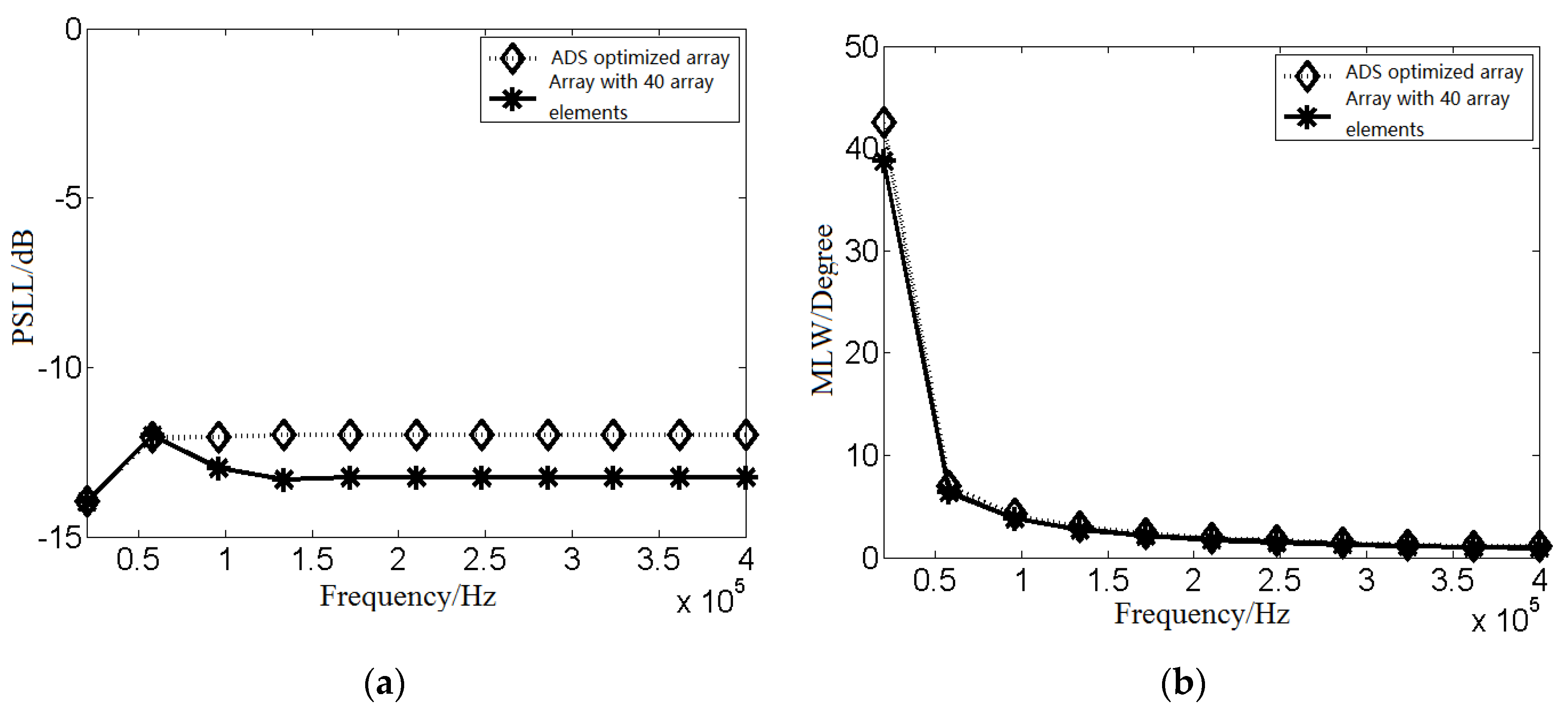
4.4. Frequency Performance

It is essential to investigate the frequency performance of the sparse array obtained via the ADS method, so that this sparse optimization method can be applied to future practical projects. Therefore, the above obtained sparse array using the (40,20,9,10)-ADS sequence structure is used to produce some frequency examinations, and the results are compared with those of the original Mills Cross array with 40 × 40 elements. The relevant parameters are set as follows: center frequency (design frequency) $f_0$ = 300 kHz, signal frequency range $f_{\min }$ = 20 kHz, $f_{\max }$ = 400 kHz, frequency step 40 kHz. Main lobe width (MLW) and PSLL are adopted as performance indices. The experimental results are shown in Figure 11. The size of array aperture is specified as $(k-1)\cdot \lambda /2$ in the simulation experiments. Otherwise, the grating lobes must appear when the wave frequency increases to a certain extent if using the fixed size of array aperture.

As shown in Figure 11, the PSLL values of the two arrays are different in the given frequency range, except for 60 kHz below, while their MLW have consistent values. The PSLL deviations are always 1.5 dB at the different frequencies. The deviations are caused by the aforementioned overlarge thinned ratio resulting from the spatial undersampling of the array sensor. This illustrates that the trends of PSLL and MLW of the sparse array after the ADS method are in line with the original Mills Cross array in the given frequency range.

5. Conclusions

This paper proposes the ADS method to further thin Mills Cross arrays while keeping the beam pattern unchanged, in order to reduce the complexity and cost of array sonar imaging systems. Simulations of the thinned arrays were conducted and compared with those of the original Mills Cross array. The results demonstrate that the PSLL values of the beam pattern are affected by the thinned ratio and the cycle number. The beam patterns do not decrease as long as the ADS parameters are correctly assigned. In addition, the MLW and PSLL values remain almost unchanged with azimuth angle and frequency variation. The azimuth resolution is maintained when using the given ADS sequence, but it is possible that the azimuth resolution is influenced by the thinned ratio. However, it is true that the azimuth resolution and the MLW are affected by the aperture size of the array sensor. From these experimental results, it is concluded that the ADS method can further decrease the redundancy of a Mills Cross array while maintaining the beam pattern. A mathematically deduced ADS sequence for Mills Cross array sensor sparse optimization will be provided in our future work.

References

1. Silkaitis, J.M.; Douglas, B.L.; Lee, H. Synthetic-aperture sonar imaging: System analysis, image formation, and motion compensation. In Proceedings of the Conference on Signals, Systems and Computers, Pacific Grove, CA, USA, 30 October–1 November 1995; pp. 423–427. [Google Scholar]
2. Hansen, E.R. Synthetic Aperture Sonar Technology Review. Mar. Technol. Soc. J. 2013, 47, 117–127. [Google Scholar] [CrossRef]
3. Repetto, S.; Palmese, M.; Trucco, A. Design and Assessment of a Low-Cost 3-D Sonar Imaging System Based on a Sparse Array. In Proceedings of the 2006 IEEE Instrumentation and Measurement Technology, Sorrento, Sorrento, Italy, 24–27 April 2006; pp. 410–415. [Google Scholar]
4. Liu, X.H.; Sun, C.; Yi, F.; Li, M. Underwater three-dimensional imaging using narrowband MIMO array. Sci. China Phys. Mech. Astron. 2013, 56, 1346–1354. [Google Scholar] [CrossRef]
5. Ha, B.V.; Zich, R.E.; Mussetta, M.; Pirinoli, P. Improved compact Genetic Algorithm for thinned array design. In Proceedings of the Antennas and Propagation (EuCAP), 2013 7th European Conference on IEEE, Gothenburg, Sweden, 8–12 April 2013; pp. 1807–1808. [Google Scholar]
6. Rodríguez, J.A.; Ares, F.; Moreno, E. Linear array pattern synthesis optimizing array element excitations using the simulated annealing technique. Microw. Opt. Technol. Lett. 2015, 23, 224–226. [Google Scholar] [CrossRef]
7. D’urso, M.; Prisco, G.; Tumolo, R.M. Maximally Sparse, Steerable, and Nonsuperdirective Array Antennas via Convex Optimizations. IEEE Trans. Antennas Propag. 2016, 64, 3840–3849. [Google Scholar] [CrossRef]
8. Yuan, Z.H.; Geng, J.P.; Jin, R.H.; Fan, Y. Pattern Synthesis of 2-D Arrays Based on a Modified Particle Swarm Optimization Algorithm. J. Electron. Inf. Technol. 2007, 29, 1236–1239. [Google Scholar]
9. Liu, X.; Zhou, F.; Zhou, H.; Tian, X.; Jiang, R.; Chen, Y. A low-complexity real-time 3-D sonar imaging system with a cross array. Ieee J. Ocean. Eng. 2015, 41, 262–273. [Google Scholar]
10. Scenario, I.T. Minimum Redundancy MIMO Array Synthesis by means of Cyclic Difference Sets. Int. J. Antennas Propag. 2013, 2013, 356–360. [Google Scholar]
11. Dong, J.; Liu, F.; Guo, Y.; Shi, R. MIMO radar array thinning optimization exploiting almost difference sets, Optik, 2016, 10, 4454-4460. Optik 2016, 10, 4454–4460. [Google Scholar] [CrossRef]
12. Luo, Y.Y.; Guo, Q.; Lutsenko, V.I.; Zheng, Y. Nonequidistant Two-Dimensional Antenna Arrays Based on the Structure of Latin Squares Taking Cyclic Difference Sets as Elements. In Proceedings of the 2019 European Microwave Conference in Central Europe (EuMCE), Prague, Czech Republic, 13–15 May 2019; pp. 427–430. [Google Scholar]
13. Carlin, M.; Oliveri, G.; Massa, A. On the Robustness to Element Failures of Linear ADS-Thinned Arrays. IEEE Trans. Antennas Propag. 2011, 59, 4849–4853. [Google Scholar]
14. Arasu, K.T.; Ding, C.; Helleseth, T.; Kumar, P.V.; Martinsen, H.M. Almost difference sets and their sequences with optimal autocorrelation. IEEE Trans. Inf. Theory 2001, 47, 2934–2943. [Google Scholar] [CrossRef]
15. Zhang, Y.; Lei, J.; Zhang, S. A new family of almost difference sets and some necessary conditions. IEEE Trans. Inf. Theory 2006, 52, 2052–2061. [Google Scholar] [CrossRef]
16. Oliveri, G.; Donelli, M.; Massa, A. Linear Array Thinning Exploiting Almost Difference Sets. IEEE Trans. Antennas Propag. 2009, 57, 3800–3812. [Google Scholar] [CrossRef] [Green Version]
17. Oliveri, G.; Massa, A. ADS-based array design for 2-D and 3-D ultrasound imaging. IEEE Trans. Ultrason. Ferroelectr. Freq. Control 2010, 57, 1568–1582. [Google Scholar] [CrossRef] [PubMed] [Green Version]
18. Oliveri, G.; Massa, A. Genetic algorithm (GA)-enhanced almost difference set (ADS)-based approach for array thinning. Microw. Antennas Propag. Iet 2015, 5, 305–315. [Google Scholar] [CrossRef]
19. Li, L.; Wang, B.; Xia, C.; Liu, X.; Cao, S. Design of Array with Multiple Interleaved Subarray based on Subarray Excitation Energy-matching. J. Beijing Univ. Aeronaut. Astronaut. 2016, 42, 2395–2402. [Google Scholar]
20. Sun, F.; Lan, P.; Gao, B.; Chen, L.A. A low complexity direction of arrival estimation algorithm by reinvestigating the sparse structure of uniform linear arrays. Prog. Electromagn. Res. C 2016, 63, 119–129. [Google Scholar] [CrossRef] [Green Version]
21. Skolnik, M. Radar Handbook, 2nd ed.; McGraw-Hill: New York, NY, USA, 2003. [Google Scholar]
Figure 1. Autocorrelation function C s ADS ( z ) of D.
Applsci 10 03176 g001
Figure 2. Mills Cross array with nine transmit and nine receive elements.
Applsci 10 03176 g002
Figure 3. Virtual array form Mills Cross array in Figure 2.
Applsci 10 03176 g003
Figure 4. Almost Different Sets (ADS) optimization procedure for a Mills Cross array.
Applsci 10 03176 g004
Figure 5. Thinned array from the Mills Cross array and the corresponding virtual array. (a) ADS thinned array form the Mills Cross array; (b) Virtual Array formed from subfigure (a).
Applsci 10 03176 g005
Figure 6. Power pattern when K = 20 , ϕ = 0 , and φ = 0 ; σ = 0, 15, and 28, respectively.
Applsci 10 03176 g006
Figure 7. 3D and 2D power patterns of the obtained sparse array after ADS. (a) θ and φ are 0°; (b) θ and φ are 0°; (c) θ and φ are 30°; (d) θ and φ are 30°; (e) θ and φ are 45°; (f) θ and φ are 45°; (g) θ and φ are 60°; (h) θ and φ are 60°; (i) θ and φ are 75°; (j) θ and φ are 75°.
Applsci 10 03176 g007aApplsci 10 03176 g007b
Figure 8. Beam power pattern of the original Mills Cross array. (a) 3D pattern; (b) 2D section pattern.
Applsci 10 03176 g008
Figure 9. Beam power pattern of the obtained array after employing the CDS method. (a) 3D pattern; (b) 2D section pattern.
Applsci 10 03176 g009
Figure 10. Azimuth resolution of four different arrays. (a) Sparse array after ADS implementation (40,20,9,10); (b) Sparse array after CDS implementation (40,21,1); (a) Sparse array after ADS implementation (40,20,9,10); (d) Mills Cross array with 20 × 20 elements.
Applsci 10 03176 g010
Figure 11. Receiving performances of two arrays at different frequencies. (a) PSLL changes at different frequencies; (b) main lobe width (MLW) changes at different frequencies.
Applsci 10 03176 g011