Abstract
As a powerful numerical analysis tool, PFC (Particle Flow Code) is widely applied to investigate the mechanical behavior of rock specimen or rock engineering under different stress states. To match the macroscopic properties of the PFC model with those of the rock, a set of micro-scale parameters of the model needs to be calibrated. Thus, this paper proposed an optimization method combining Box–Behnken experimental design and desirability function approach to quickly and accurately find the values of the micro-scale parameters. The sensitivity of the main micro-scale parameters (mean value of parallel-bond normal strength σc, ratio of particle normal to shear stiffness Ec, and Young’s modulus at each particle–particle contact kn/ks) and their interactions to the macroscopic responses (uniaxial compressive strength, Young’s modulus, and Poisson’s ratio) were thoroughly analyzed using response surface theory. After that, validation study was conducted on the calibrated model. The results manifest that the uniaxial compressive strength is extremely significantly affected by σc and kn/ks, the Young’s modulus is highly correlated with Ec and kn/ks, and the Poisson’s ratio is most significantly influenced by kn/ks. Additionally, the interaction of micro-scale parameters also has different impact upon the responses. Moreover, the simulated crack behavior around differently shaped openings in rock samples under uniaxial compression is found to be well agreeable with the experimental results, which verifies the reliability of the proposed method.
1. Introduction
With the rapid development of information technology and computational mechanics theory, more and more commercial software based on finite element method (FEM), discrete element method (DEM), boundary element method (BEM), or finite difference method (FDM) has been developed [1,2,3,4,5,6], such as Abaqus [7], Ansys [8,9], FLAC (Fast Lagrangian Analysis of Continua) [10,11], Rocscience [12], UDEC (Universal Distinct Element Code) [13], and PFC (Particle Flow Code) [14]. Since these pieces of software possess significant merits like low cost, high efficiency, and broad range of applications [15,16,17], they have been widely applied to investigate both the macroscopic and microscopic mechanical behavior of large-scale rock engineering or small-size rock specimens.
DEM is a numerical solution devoted to describing the mechanical behavior of discontinuous media, particularly the rock and rock-like materials. Inspired by molecular dynamics method, Cundall [18] first proposed a DEM model to simulate the gradual motion of blocky rock mass. Afterwards, it was employed to study the mechanical characteristics of granular assemblies, and the results indicated that the obtained force vector plots by a computer program show good agreement with those from photoelastic disc tests [19]. Later on, a series of versions of DEM-based PFC software was released by Itasca Consulting Group, Inc. This piece of promising software has a wide range of applications, e.g., slope stability, rock fracture, underground mining, hydraulic fracturing, and flow simulation.
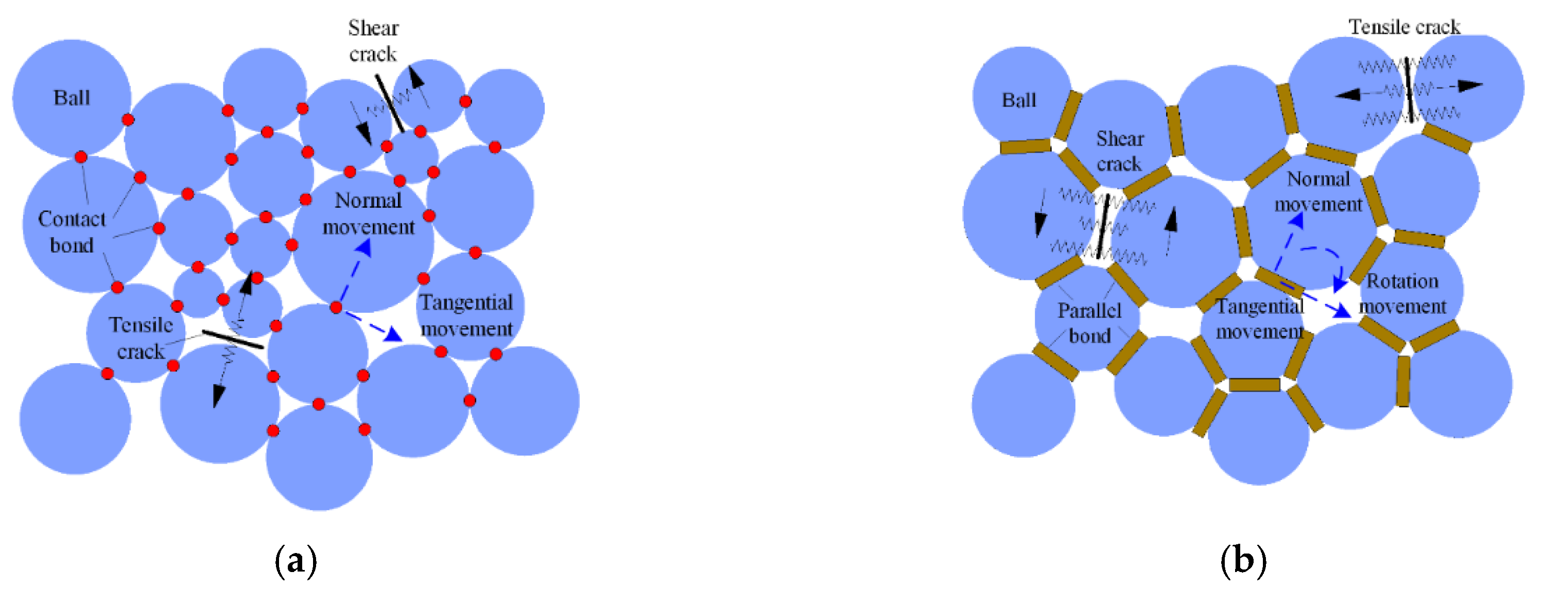
In PFC model, the medium is idealized as an assembly of various sized rigid particles and the bonds between them. The motion and interaction of the particles affect the macromechanical behavior. The shape of the particles is circular in PFC2D (Two-dimensional PFC) and spherical in PFC3D (Three-dimensional PFC). There are two types of bonds: contact bond and parallel bond [20] (Figure 1). For the contact-bond model, the adjacent particles are connected by point-formed bonds; that is, the particles can only move in translation and not in rotation. As long as the particles are in contact, the contact stiffness remains the same regardless of whether the bond is broken [21]. Clearly, this is not realistic in rock mechanics. With regard to the parallel-bond model, particles are contacted via a bond with a certain thickness and radius. When particles translate or rotate, both the force and moment can be transmitted through the bond. Once the normal or tangential stress on the bond exceeds its normal or tangential strength, fracture will occur as tensile or shear cracks. This behavior is consistent with the actual fracture of the rock. Hence the parallel-bond model was selected for PFC modeling in this study. During modeling, the macroscopic physical and mechanical properties as well as the constitutive model of the material are not required to predefine. The reason is that the mechanical response is controlled by the motion and interaction of the particles. Thus, determining a set of micro-scaled physical and mechanical parameters of the particle and contact to match the macro-response of the material is essential. Obviously, the accuracy of PFC simulation is strongly associated with these parameters.
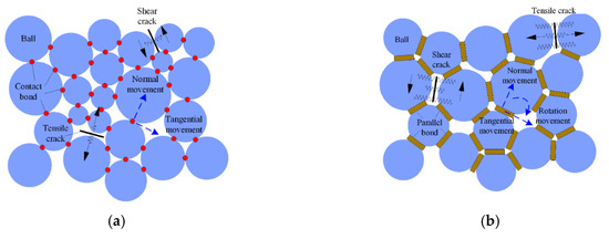
Figure 1.
Type of bond model: (a) contact-bond model and (b) parallel-bond model.
Currently, the trial-and-error method is commonly used to calibrate the micro-scale parameters of the PFC model based on uniaxial compression test results of rock specimens; that is, they need to repeat performing uniaxial compression simulation by adjusting these parameters until the simulated uniaxial compressive strength, elastic modulus, Poisson’s ratio, and failure mode of the model are consistent with the laboratory test results. Indeed, the number of the micro-scale parameters is quite large, and determining a proper set of micro-scale parameter values is extremely time consuming and troublesome. Therefore, it is meaningful to find an approach to address this issue quickly and reliably. To explore the relationship between micro-scale parameters and macroscopic mechanical properties, a few attempts have been made by some researchers. Yoon [22] applied the Plackett–Burman design method to analyze the sensitivities of micro-scale parameters to macro-response of contact-bond model, and singled out two most significant micro-scale parameters for each macroscopic property. By using Taguchi method, Hanley et al. [23] performed a calibration on micro-structural parameters of parallel-bonded agglomerates in both 2D and 3D models. It is found that the normal strength of bond, bond stiffness, and particle friction are the dominant parameters influencing the strain at failure. Cheung et al. [24] conducted a parametric study to identify the effect of parallel bond-contact stiffness ratio, bond area, and bond strength on stress–strain response of PFC3D model. Results show that the overall stiffness increases with the increase of the first two parameters, but is not affected by the bond strength. Shi et al. [25] summarized that the macroscopic Young’s modulus is controlled by the modulus of the bond and particle, the Poisson’s ratio depends on the ratio of particle normal to shear stiffness, and the uniaxial compressive strength is related to the bond shear strength. Also, the linear equations between them are fitted. Castro-Filgueira et al. [26] argued that bond cohesion has a remarkable impact on the model strength. Ding et al. [27] further examined the effects of maximum to minimum particle size ratio and particle size distribution on the macroscopic mechanical properties of PFC3D, which show good agreement with the results of Wang et al. [28] using similitude rules. Besides, based on numerous uniaxial compression simulations, Tawadrous et al. [29] utilized artificial neural networks to predict the micro-properties required for PFC3D modeling under three given macro-properties. By means of gray relational analysis and factorial screening, Zou and Lin [30] obtained the dominant micro- parameters influencing the uniaxial compressive strength, Young’s modulus, and Poisson’s ratio of coal. Moreover, Wang and Cao [31] used an improved simulated annealing algorithm to find the approximate values of these micro-parameters, which does not require establishing the relationship between microscopic and macroscopic parameters. Sun et al. [32] further developed FFD-ANN (Full Factorial Designs and Artificial Neural Networks) method to predict the micro-parameters of PFC3D model for triaxial compression tests.
From the literature review, it can be concluded that relationship between partial micro- and macro- parameters has been revealed. However, so far, it is still unclear that how these parameters interact with each other and collectively affect each macro-scaled mechanical property. Moreover, information regarding effective methods for finding the micro-scale parameters quickly is relatively rare. Therefore, in this research, a novel experimental design method incorporating Box–Behnken response surface methodology and desirability function optimization (BB-DFO) approach was proposed to conduct sensitivity analysis and optimization of micro-scale parameters of parallel-bond model. After that, the fracture development around circular, square, and D-shaped openings in rock specimens loaded in uniaxial compression was simulated using the calibrated PFC model and then was compared with the results of experimental investigation.
2. Microscopic and Macroscopic Parameters of PFC Model
2.1. Key Microscopic Parameters of Parallel-Bond Model
In this study, the main purpose is to find an approach to determine the micro-scale parameters of parallel-bond model, which can be used to simulate fracture propagation in rock specimens under uniaxial loads. As the internal fracture in thin specimens can be well represented by the surface cracks, the rock specimens used for lab tests are usually machined into prisms. Accordingly, the PFC2D software is commonly adopted to study the rock fracture behavior [33]. The microscopic parameters of the parallel-bond model can be classified as: specimen-genesis control parameters, particle-based material parameters, and parallel-bond parameters. To avoid boundary effects, dimensions of the rock model were set to 100 mm in width and 150 mm in length. The final platen velocity, namely, axial loading speed, was maintained at 0.05 m/s, and the test-termination criterion was assigned a value of 0.6. For the other specimen-genesis control parameters, their values were default according to the PFC manual [34]. Besides, Table 1 shows the detailed descriptions concerning the parameters of the particle and the bond.

Table 1.
Main microscopic parameters of parallel-bond model.
Table 1 shows that the slope of the post-peak stress–strain curve is closely related to the particle friction coefficient. After several trial and error attempts, its value can be easily determined based on the experimental stress–strain curve. Overall, the uniaxial compressive strength of the model is controlled by σc, τc, , and , the Young’s modulus is jointly influenced by Ec and , and the Poisson’s ratio is highly correlated with kn/ks and [35,36,37]. Besides, interactions between the micro-scale parameters also affect them to varying degrees [24]. In respect of and , they are used for small-scale adjustments and have little impact on the macro-mechanical properties. To quickly determine the values of these parameters, the following simplifications are made: σc = τc, Ec = , and kn/ks = [36]. Therefore, the number of independent variables to be optimized are reduced to three, i.e., σc, Ec, and kn/ks.
2.2. Measurement of Macroscopic Mechanical Parameters
The macroscopic parameters of the parallel-bond model for uniaxial compression simulation include uniaxial compressive strength, Young’s modulus, and Poisson’s ratio. Since the PFC model used for rock fracture analysis is two dimensional, three prismatic sandstone specimens (length × width × height = 100 mm × 25 mm × 150 mm) were first made and tested in uniaxial compression. According to the stress–strain curves, the average values of the uniaxial compressive strength and Young’s modulus were 102.61 MPa and 20.78 GPa, respectively. Due to the difficulty in measuring the Poisson’s ratio of the prismatic specimens, three other cylindrical specimens with a diameter of 50 mm and a height 100 mm were further prepared for uniaxial compression tests, which were conducted by MTS (Mechanical Testing & Simulation) 815 rock mechanics testing machine. The Poisson’s ratio, calculated from the axial strain and hoop strain measured by the axial and hoop strain extensometers, was 0.258.
3. BB-DFO Experimental Design Method
3.1. Box–Behnken Response Surface Approach
One of the important purposes of data analysis is to study the relationship between things and discover the potential laws. Generally, these objective regularities are often affected by various factors. Therefore, to reduce the error of analysis results and improve the efficiency at the same time, carrying out reasonable experimental design is indispensable. Otherwise, it will not only increase the number of experiments, prolong the experiment cycle, and cause waste of manpower, materials, and time but also give rise to unexpected results or even result in the entire study to fail. Response surface methodology, proposed by Box and Wilson [38], is a mathematical statistical method to solve nonlinear optimization problems. By using this method, it is able to obtain not only the functional relationship between multiple influencing factors and each response variable but also the interaction between different influencing factors. The basic principle of this method is to find a response surface function = f(x) that can approximate the mapping function y = f(x) between the independent variable x and the dependent variable y through experimental design, so that the response variable → y. Afterwards, the response surface function is optimized according to the constraints, and then the independent variable can be solved.
Currently, response surface function has evolved from first-order linear functions to higher order polynomial functions that take into account the interaction between independent variables. The commonly used second-order response surface function can be expressed as
where represents the predicted response variable, xi denotes the independent variable, and n means the number of independent variables. β0, βi, βij, and βii (i, j = 1, 2,···, n) are unknown constants which can be determined iteratively from test sample points, and the total number is (n + 1)(n + 2)/2.
Provided that m trials were performed, the expression of the response surface variable can be written as
where Y, X, β, and ε denote vectors of dependent variables, independent variable, constant, and error, respectively, namely,
To find the response surface closest to all experimental data points, the least squares method is used to minimize the sum of the squares of ε, that is,
Let ΔS(β) = 0, the following equation can be obtained by simplification.
Based upon the test sample data, the constant β can be solved according to Equation (5), and then the response surface function can be easily found by substituting them into Equation (1). From the above, the design of experiment is the premise of applying the response surface methodology to find the response surface function and analyze the significance of the independent variables. At present, the commonly used experimental design methods include completely random design, paired block design, Latin square design, orthogonal experimental design, uniform experimental design, and factorial experimental design. As there is no axial point, Box–Behnken design that is particularly suitable for three-factor situation requires less experiments than other design methods. Thus, it was employed to design the experimental scheme in this study.
3.2. Desirability Function Optimization Method
Actually, the response surface methodology is only applicable to optimizing single response variable. If multiple responses are required to optimize at the same time, the global solution of the independent variables cannot be derived directly using this method. Consequently, it is necessary to develop a multi-objective optimization approach. For this purpose, a desirability function method proposed by Candioti et al. [39] was used to optimize the micro-scale parameters of PFC model. The individual desirability function of a response variable can be expressed as
where dj(ŷj) (j = 1, 2, 3,…, K) denotes the desirability of the response variable ŷj whose value is between 0 to 1; dj(ŷj) = 0 means poor response and dj(ŷj) = 1 stands for ideal response. Lj, Uj, and Tj represent the lower limit, upper limit, and optimal target value of the response variable, respectively. s and t are the weights set by the analyst to determine how important they are for ŷi to be close to the maximum and the minimum, respectively. In this work, their values were both set to 1.
Note that Equation (6) is suitable for the larger-the-better typed response variable, which indicates that the larger the response variable is, the higher the desirability will be. For Equation (7), the situation is opposite. By contrast, Equation (8) is applicable to the situation where the specific target value is required; that is, the closer the response variable to the set target value, the higher the desirability. Thus, the overall desirability of the multiple response variables can be calculated using the following equation:
where D is the overall desirability of the response variables. Clearly, the closer D is to 1, the more satisfactory is the result. rj (j = 1, 2, 3,…, K) is the importance of each response variable relative to the others, with a value ranging from 1 to 5. The larger the value, the more significant the response variable.
In this study, there are three independent variables (σc, Ec, and kn/ks, denoted by A, B, and C, respectively) and three response variables (uniaxial compressive strength y1, Young’s modulus y2, and Poisson’s ratio y3). In other words, we need to determine the values of A, B, and C by the proposed BB-DFO experimental design method based on the laboratory test results of y1, y2, and y3. Figure 2 illustrates the technical route of multi-objective optimization of these micro-scale parameters, which is composed of four parts: design of experiment, modeling, analysis of variance, and multiple optimization.

Figure 2.
Technical route of determination of micro-scale parameters using Box–Behnken response surface methodology and desirability function optimization (BB-DFO) method.
4. Experimental Design and Analysis
4.1. Experimental Scheme and Results
As stated above, three influencing factors and three response variables were considered in this study. Hence, a three-level-three-factor model was established using Box–Behnken design. According to the laboratory test results, the defined levels of each factor are given in Table 2. To make statistical calculation simple, dimensionless processing was conducted on these factors according to
where Xi and xi (i = 1, 2, and 3) denote the dimensionless coded value and actual value of influencing factor, respectively, x0 is the actual value of the factor at the center point, and Δxi means the step change value of the influencing factor.

Table 2.
Ranges of influencing factors.
According to the Box–Behnken design scheme, a total of 17 groups of uniaxial compression simulations were carried out by the PFC software. Table 3 shows the simulation results. Accordingly, different models, including the linear, 2FI (Two-Factor Interaction), quadratic, and cubic models were employed to fit the second-order response surface equation. Lack-of-fit test results indicate that the quadratic model fits well the nonlinear relationship between the independent and dependent variables (see Table 4). It is noted that the cubic model and higher are aliased. The fitted equations of the response variables with respect to the actual factors are given as

Table 3.
Box–Behnken design scheme and results.

Table 4.
Model summary statistics.
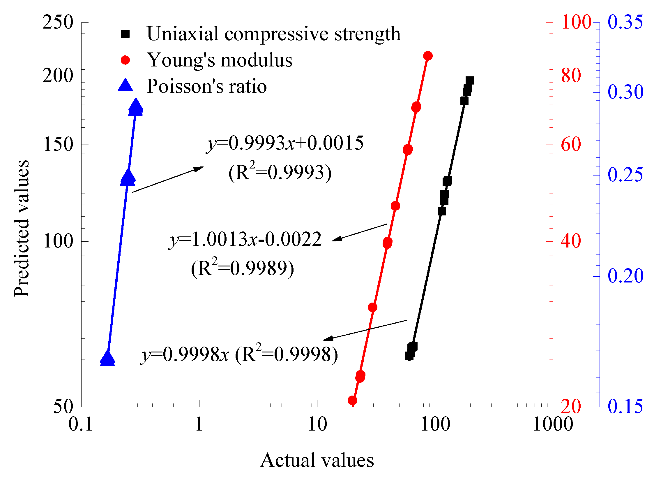
Equations (11)−(13) show that all the correlation coefficients are greater than 0.99, suggesting that the fitted response surface functions are reliable. Also, the predicted values of the response variables are found to be extremely agreeable with the simulated results (Figure 3). The average prediction errors of the uniaxial compressive strength, Young’s modulus, and Poisson’s ratio reach 0.70%, 0.85%, and 0.21%, respectively.
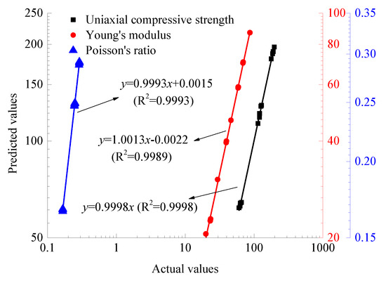
Figure 3.
Comparison of predicted and actual values of response variables.
4.2. Analysis of Variance
To further identify the significance of A, B, and C as well as their interactions on y1, y2, and y3, analysis of variance was performed on each response variable model. In general, the significance of the model terms can be evaluated on the basis of F-value and p-value. It is calculated that the F-values of the three models are 1480.09, 1372.12, and 3553.51, respectively, all of which are greater than F0.95(8,8) = 3.438. For the p-values, they are all less than 0.0001. This implies that these fitted models are extremely significant. Note that the larger the F-value or the smaller the p-value is, the more significant the model will be. With regard to the probability of the model term, p < 0.0001, p < 0.05, and p > 0.05 means it is extremely significant, significant, and insignificant, respectively. Also, the signal-to-noise ratios of the three models are 113.49, 131.69, and 163.63, respectively, which are much larger than 4. Clearly, these models with adequate signals can be applied to navigate the design space. Moreover, their coefficients of variation are 1.23%, 1.38%, and 0.42%, respectively, indicating that the models have high accuracy.
4.2.1. Influence of Micro-Scale Parameters on Uniaxial Compressive Strength
Table 5 shows that the effects of A and C on uniaxial compressive strength are extremely significant, while that of B is not significant. As the value of A increases, the uniaxial compressive strength increases linearly and significantly. By contrast, the uniaxial compressive strength increases slowly with the increase of C, but the factor B has little effect on the uniaxial compressive strength (see Figure 4a). When the coded values of B and C are both zero, the uniaxial compressive strength (192 MPa) when A is 1 is found to be 2.87 times that (67 MPa) when it is −1. Within the range of B, the strength changes from 120 to 130 MPa. It can be observed that the effect of A on uniaxial compressive strength is more significant than that of C.

Table 5.
Analysis of variance for quadratic response variable models.
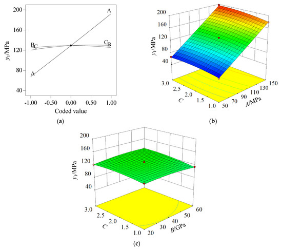
Figure 4.
Influence of micro-scale parameters on uniaxial compressive strength: (a) one-factor effect, (b) interaction effect between A and C, and (c) interaction effect between B and C.
According to the p-value obtained from the analysis of variance, it is further found that the interactions between A and C and between B and C have a significant effect on the uniaxial compressive strength, which are illustrated in Figure 4b,c. Figure 4b shows that the uniaxial compressive strength increases as A and C increase simultaneously. The response surface plot also verifies that A has a greater influence on intensity than C. Further on, the strength is also significantly affected by the interaction between B and C (see Figure 4c). When the coded values of B and C are near zero, the uniaxial compressive strength has a maximum value.
4.2.2. Influence of Micro-Scale Parameters on Young’s Modulus
Similarly, we can obtain the impact of these three micro-scale parameters on the macroscopic Young’s modulus. Figure 5 clearly demonstrates the one-factor and multiple factor interaction effects. The influence of B and C on Young’s modulus are extremely significant, while A does not affect it significantly. The Young’s modulus linearly changes from 22 to 70 GPa as the coded value of B increases from −1 to 1. When C varies from −1 to 1, the Young’s modulus decreases nonlinearly from 59 to 40 MPa, the reduction rate gradually decreases. Besides, it is found that the interaction between B and C has an extremely significant effect on the Young’s modulus, whereas the interactions of A–B and A–C are not significant. With the rise of B and the decrease of C, the Young’s modulus gradually increases.
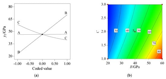
Figure 5.
Influence of micro-scale parameters on Young’s modulus: (a) one-factor effect and (b) interaction effect between B and C.
4.2.3. Influence of Micro-Scale Parameters on Poisson’s Ratio
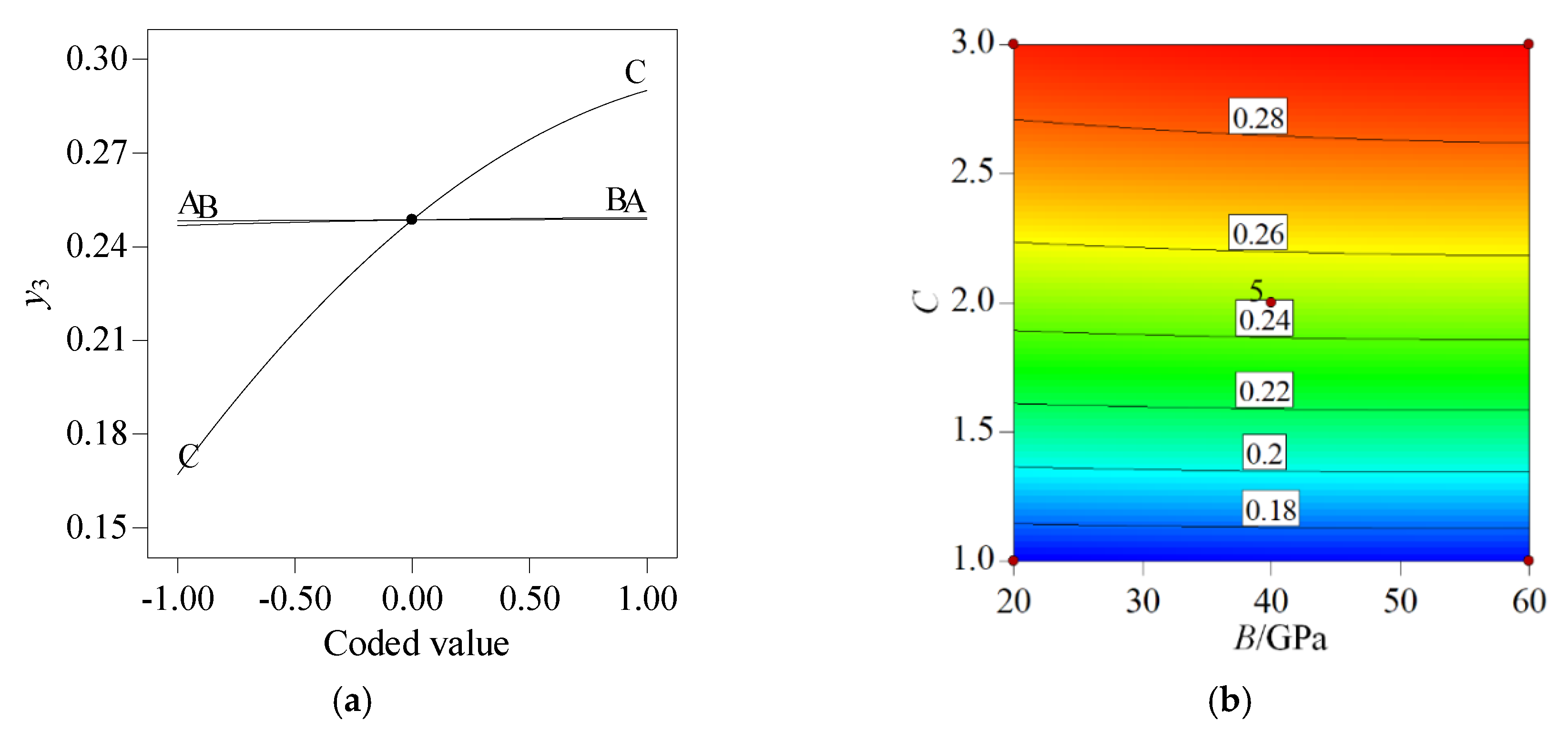
The effects of A, B, and C and their interactions on the Poisson’s ratio can also be derived based on the results of the analysis of variable. Figure 6a shows that the influence of B and C on the Poisson’s ratio are significant and extremely significant, respectively, while that of A is not remarkable. The Poisson’s ratio increases slowly with the increase of B, but grows first sharply and then slowly as C rises. Within the range of C, the minimum and maximum Poisson’s ratios are 0.16 and 0.29, respectively, with an increase rate of 81.25%. By contrast, with the increase of B, the increase of Young’s modulus is very small, and basically remains unchanged at 0.25. For the effect of the interaction, it is observed that there are no significant interactions between A and B and between A and C. The p-value of the B–C interaction is 0.3506, implying that it is also not significant. Figure 6b displays that the contours of the Poisson’s ratio are approximately horizontal.

Figure 6.
Influence of micro-scale parameters on Poisson’s ratio: (a) one-factor effect and (b) interaction effect between B and C.
4.3. Optimization of Micro-Scale Parameters
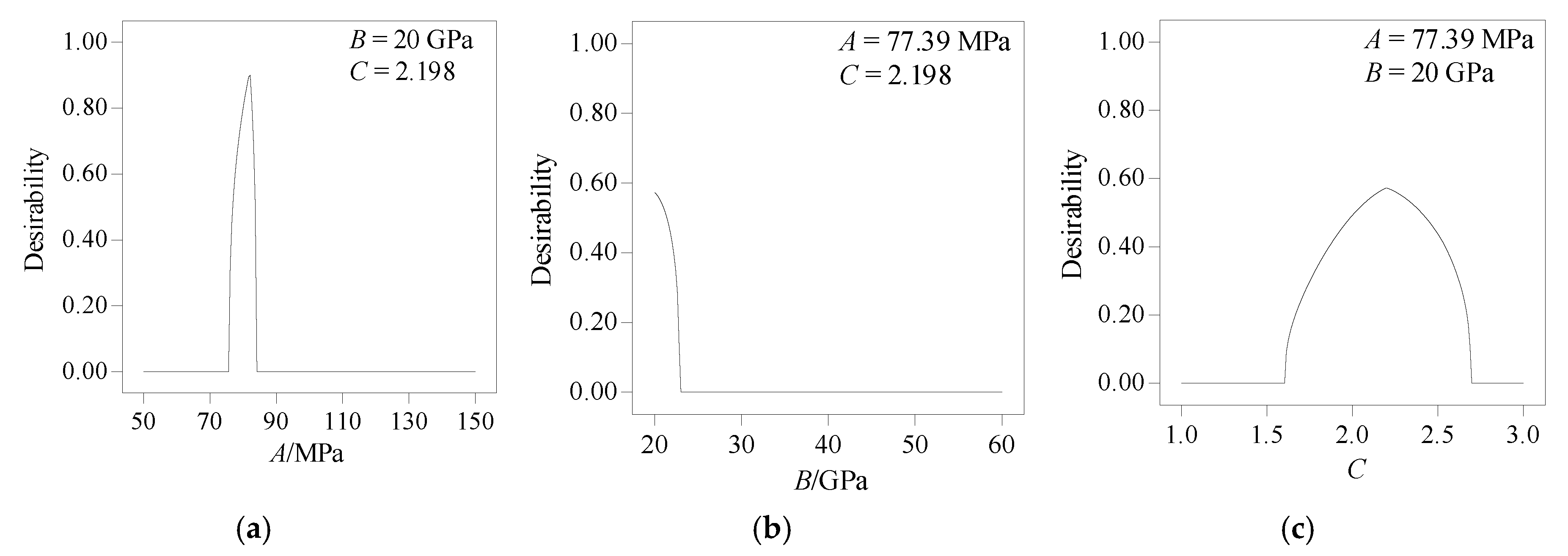
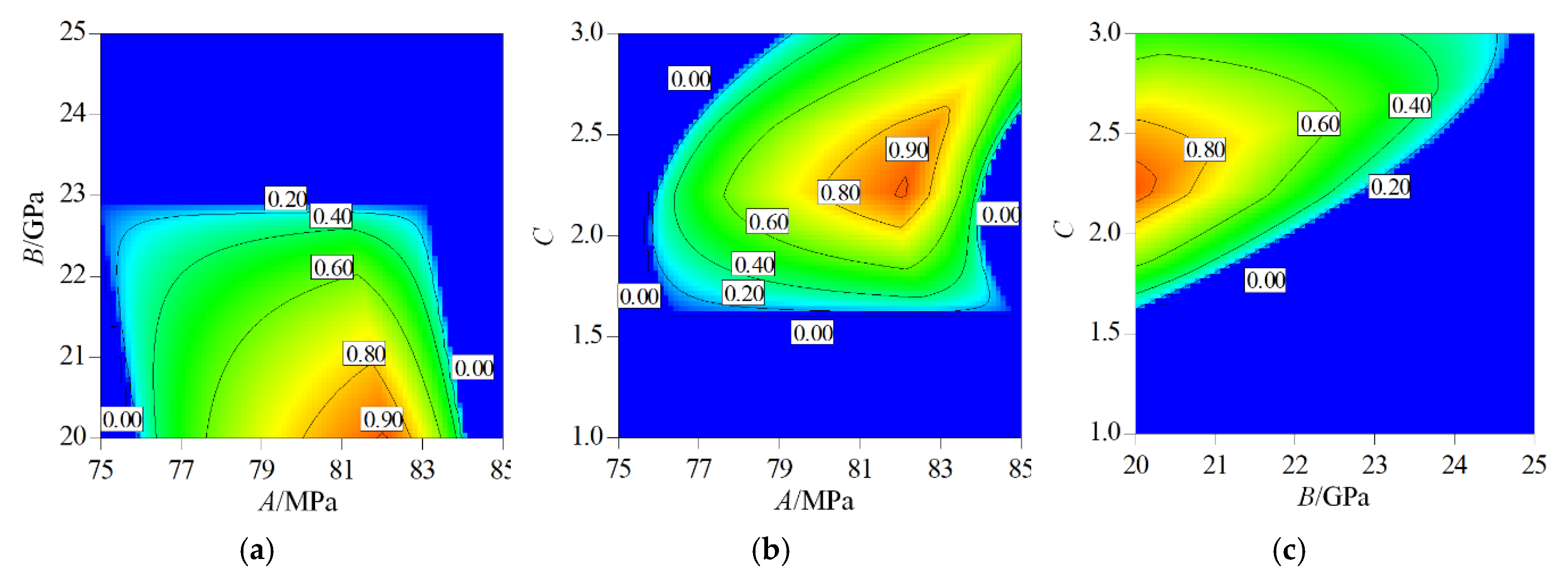
According to the principle of the desirability function method, first, we need to determine the optimization interval for each factor. The purpose of this study is to find the micro-scale parameters to fit the macroscopic mechanical response. Therefore, Equation (8) was utilized to calculate the individual desirability, and then the overall desirability could be obtained according to Equation (9). Assuming these three factors are equally important, their weights were all set to 5 (r1 = r2 = r3 = 5). The optimization intervals of A, B, and C were defined as (50,150), (20,60) and (1,3), respectively, and their target values were set to be equal to those of the uniaxial compression test results, i.e., y1 = 102.61 MPa, y2 = 20.78 GPa, and y3 = 0.258. The effect of each factor on the overall desirability is plotted in Figure 7. It is shown that the desirability is the maximum when A is 75~85 MPa, B is 20~23 GPa, and C is 1.6~2.7. In these intervals, the desirability increases first and then decrease with the increasing A and C, while it declines as B increases. Moreover, Figure 8 illustrates that the interactions between these factors have a significant effect on the overall desirability. It can be observed clearly that the overall desirability is the largest under the condition of A is about 82 MPa, B is about 20 GPa, and C is about 2.2.
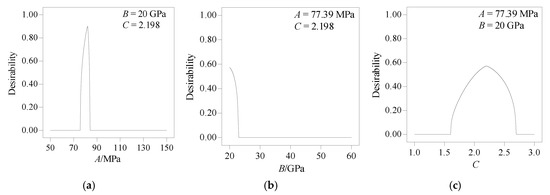
Figure 7.
Effect of one factor on overall desirability: (a) factor A, (b) factor B, and (c) factor C.
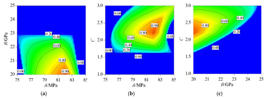
Figure 8.
Interaction effect of multiple factors on overall desirability: (a) A–B, (b) A–C, and (c) B–C.
Through optimization, we found that the overall desirability of the solution that A = 82.07 MPa, B = 20.00 GPa, and C = 2.198 is the maximum, namely, D = 0.914. In such a case, the simulated uniaxial compressive strength, Young’s modulus, and Poisson’s ratio are 102.61 MPa, 21.77 GPa, and 0.258, respectively, which are exceedingly agreeable with the laboratory results.
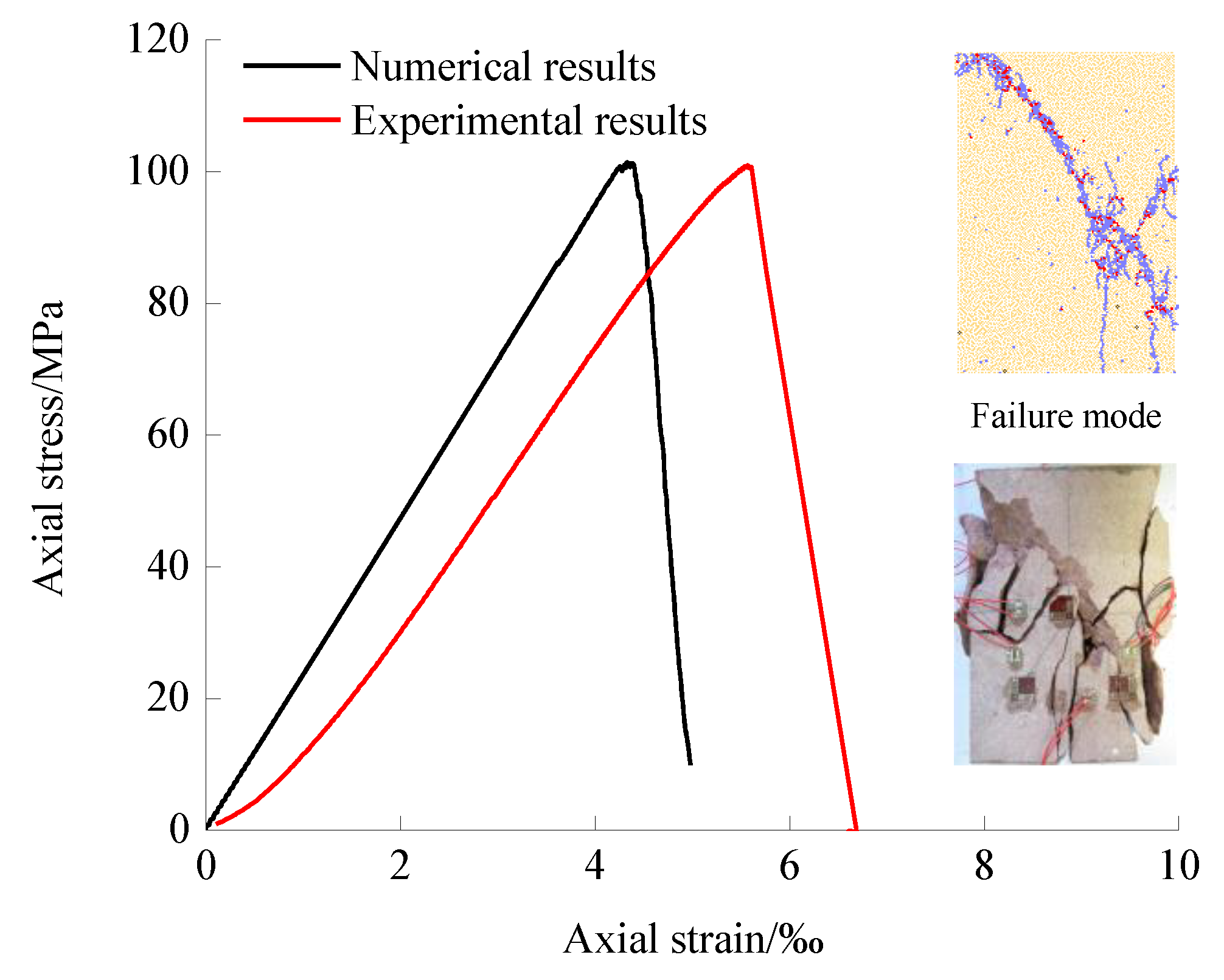
In addition to the simulated responses being consistent with laboratory test results, the failure mode of the model should also coincide with that of the rock specimen. Thus, minor adjustments are required on these parameters and the standard deviations of normal and shear strength ( and ). The final micro-scale parameters obtained are shown in Table 6, and the comparison between experimental and numerical stress–strain curves is presented in Figure 9. The peak stresses and slopes of the two curves are basically equal, with relative errors of 1.19% and 5.92%, respectively. This indicates that the uniaxial compressive strength and Young’s modulus are consistent. Since the built models compressed by two discs are strictly two dimensional, there is no initial pores and cracks compaction stage during the loading process. Consequently, the peak stain of the model is slightly smaller than that of the real rock specimen.

Table 6.
Main micro-scale parameters of parallel-bond model for rock model.

Figure 9.
Comparison between experimental and numerical stress–strain curves.
5. Application of Calibrated Model to Rock Fracture and Experimental Validation
5.1. Stress–Strain Curves
In rock mechanics and rock engineering, a good many of rock disasters like rock burst, water gushing-out, surrounding rock instability happen frequently in underground excavation at great depth [40,41,42,43,44,45]. Thus, it is critical to examine the failure process of opening under compressive stress. On the other hand, the accuracy of the micro-scale parameters can be verified. Hence, we adopted the calibrated PFC model to simulate the fracturing behavior around circular, square, and D-shaped openings in prismatic samples (length × thickness × width = 100 mm × 25 mm × 150 mm) subjected to uniaxial compression. After that, the numerical results were compared with the experimental results. In the laboratory tests, the selected rock material was still the red sandstone which came from Shandong province of China. A total of nine specimens were made, including three specimens with a circular opening (radius = 10 mm, marked as SC), three specimens with a square opening (length × width = 17.72 mm × 17.72 mm, marked as SS), and three specimens with a D-shaped opening (length × width = 16.59 mm × 22.11 mm, marked as SD) (Figure 10). To better understand the impact of the opening shape on fracturing response, the cross-sectional areas of the three openings excavated by high-pressure water cutter were designed to be equal. Further on, the aforementioned three intact samples, which were named IS, served as a reference. Uniaxial compression experiments were conducted on these three types of preholed samples under the same loading conditions as the above intact sandstone samples.
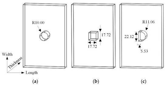
Figure 10.
Fabricated sandstone samples: (a) samples containing a circular opening; (b) samples containing a square opening, and (c) samples containing a D-shaped opening.
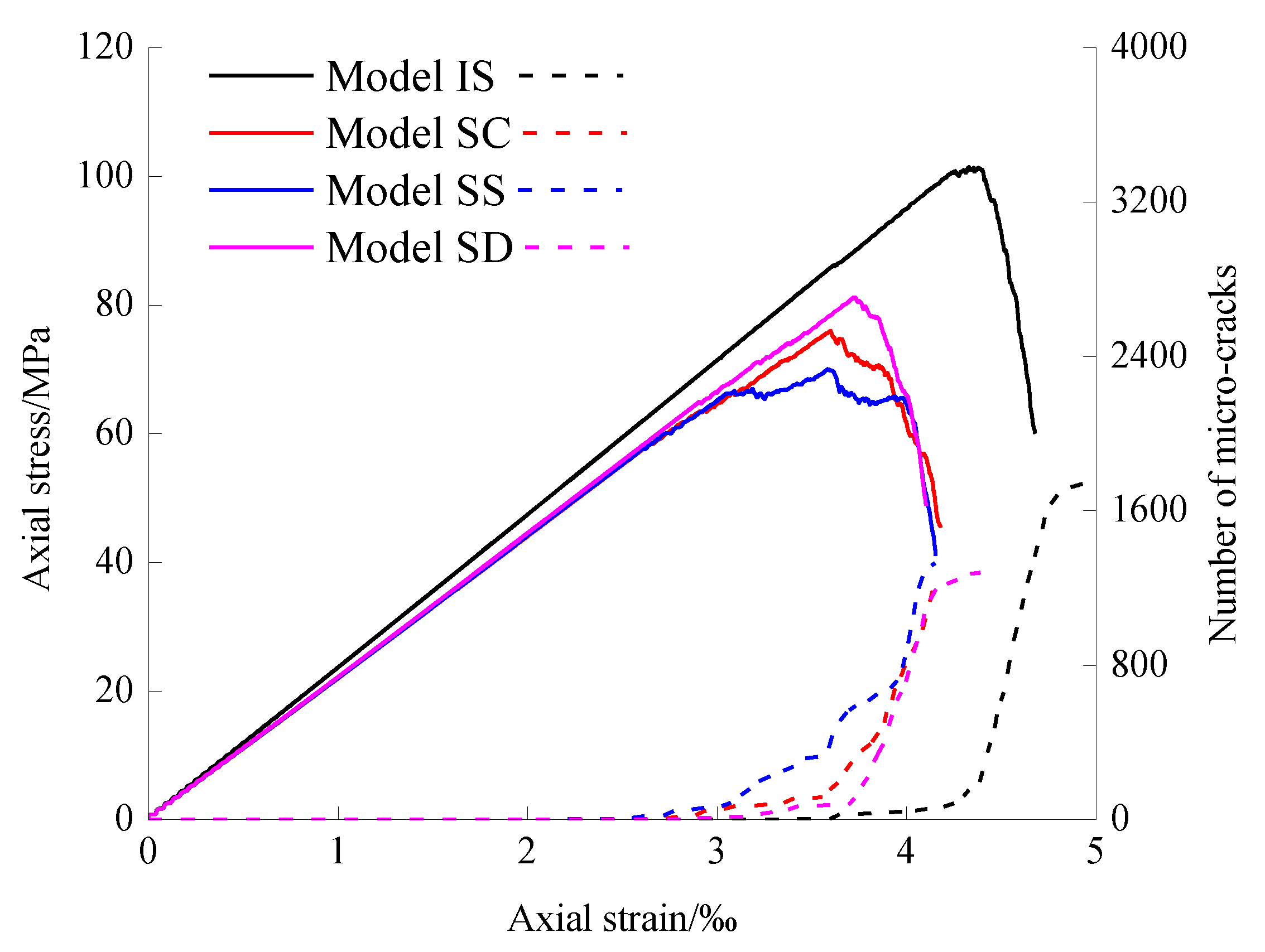
Correspondingly, three models of the same size and type as the sandstone samples with an opening were created and numerically loaded in uniaxial compression. The achieved curves of axial stress versus axial strain of these models are plotted in Figure 11. It can be seen that the axial strain of the intact model grows linearly as the axial stress increases firstly. When the axial stress approaches the peak, the curve of the intact model becomes concave down. This means that the plastic deformation starts to occur. In regard to the curves of the models with an opening, a noticeable fluctuation appears before the peak, which is induced by the sudden appearance of the cracks near the openings. Figure 11 also demonstrates the development of the number of the micro-scale cracks in the models during the numerical loading simulation. When the axial strain is very small, the number of the micro-scale cracks is limited. It is because there are a few cracks in the first two loading stages, i.e., initial pores and fissures compaction stage and linear elastic stage. Once the plastic deformation stage is reached, the micro-cracks begin to initiate and propagate drastically. As a result, the quantity of the formed micro-cracks grows significantly and the stress–strain curves at this point goes up, and then the stress decreases rapidly for the IS and SC models. After the peak, the number of the micro-cracks rises rapidly due to the coalescence of the cracks. The slopes of the curves after the peak are large, indicating that the models are quite brittle. It is further observed that the remarkable increase in the number of the micro-scale cracks of the models containing an opening occurs earlier than that of the intact model. The reason is that cracks are more likely to emerge at the stress concentration areas around the openings under loads.
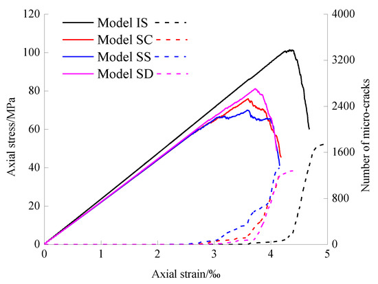
Figure 11.
Curves of axial stress versus axial strain by numerical method.
Table 7 lists the simulated uniaxial compress strength, Young’s modulus, and peak strain of the models subjected to uniaxial compression. It is observed that the strength of the models embedded an opening is much lower than that of the intact model, and the weakening degree ranging from 21.14%~31.97% is closely associated with the opening shape. Among the preholed samples, the uniaxial compressive strength of the model SD with a height–width ratio greater than 1 is the largest, while that of the model SS is the smallest. Interestingly, the strength of the model SD is larger than that of the model SC, which may be related to the height–width ratio. For the Young’s modulus, the value of the preholed samples is slightly lower than that of the intact model, and the opening shape has little influence on it. Moreover, the peak strain of the preholed models decreases significantly compared with that of the intact model, but the difference in peak strain among the preholed models is not significant.

Table 7.
Mechanical parameters of models under uniaxial compression.
5.2. Crack Development around Openings
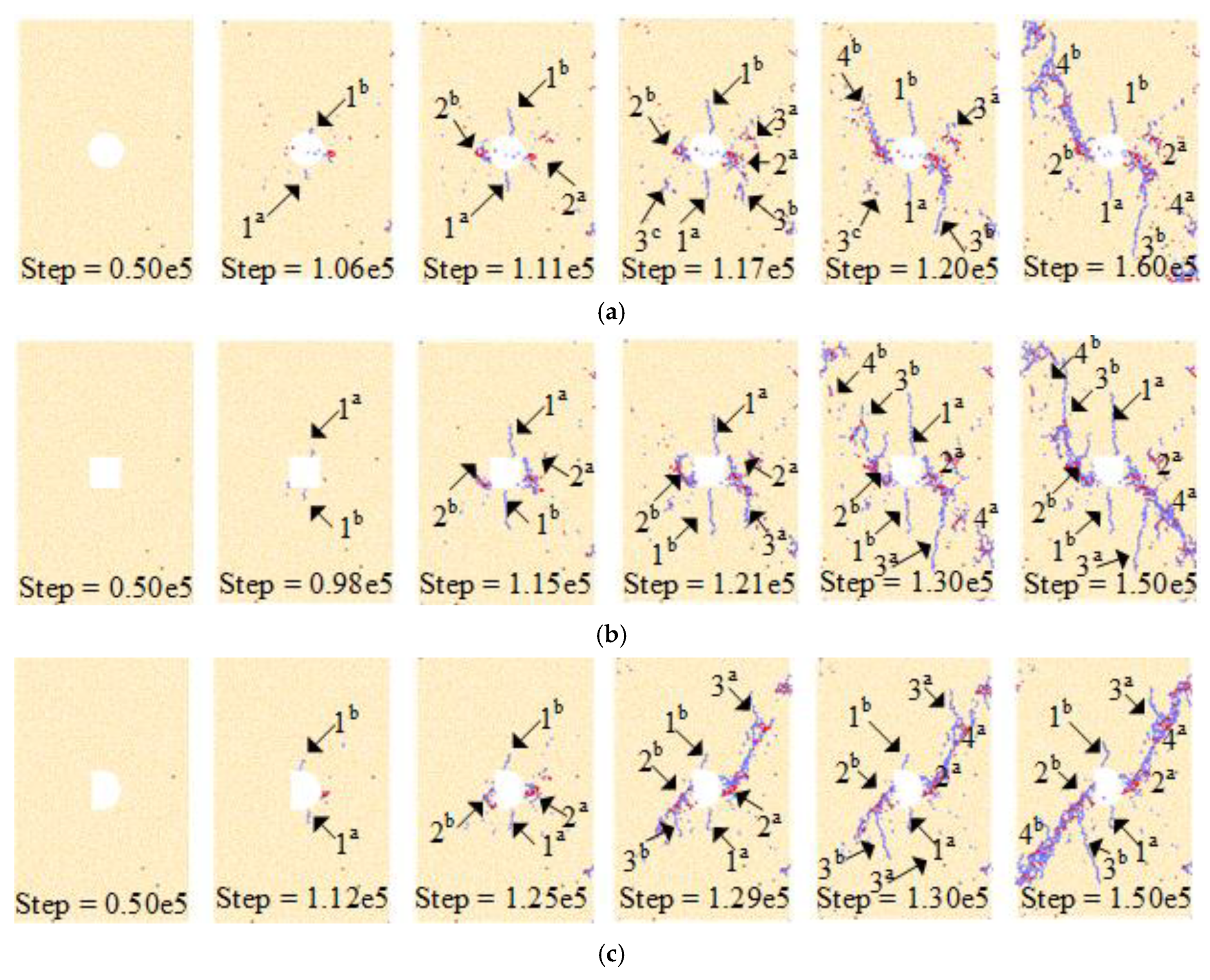
By using the calibrated PFC model, the simulated failure processes of the above three kinds of models containing an opening in uniaxial loading are shown in Figure 12. As the calculation step rises, four different types of cracks are observed in the vicinity of the openings. In terms of the model with a circular opening, no cracks are found near the opening in the elastic deformation stage. When the number of calculation steps is 1.06 × 10⁵, two cracks 1a and 1b propagating in the vertical direction are observed symmetrically at the top and bottom of the opening. After that, two exfoliation cracks 2a and 2b caused by spalling failure are formed on the left and right sidewalls of the opening, respectively. When the number of steps reaches 1.17 × 10⁵, it is seen that two cracks 3a and 3b occur on the upper-right and lower-left corners of the opening, respectively. They propagate rapidly parallel to the direction of loading until they get connected with the opening. With the further increase of the calculation step, two shear cracks 4a and 4b appear in turn on one diagonal of the model. If the shear cracks extend to the opening, the model fails immediately. Since the cracks 1 and 3 are both induced by concentrated tensile stress, we hereby define them as initial-tensile cracks and secondary-tensile cracks, respectively. With regard to the exfoliation crack 2, they are caused by the concentrated compressive stress. In contrast, the shear cracks are attributed to the high shear stress along the diagonal, which is formed by the coupling of end friction and applied load.
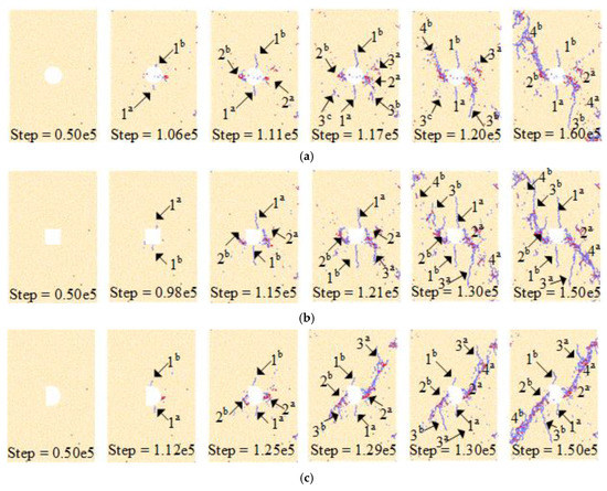
Figure 12.
Crack development around openings of different shapes under uniaxial loading obtained by numerical method: (a) model SC, (b) model SS, and (c) model SD.
Similarly, Figure 12 also illustrates the fracture responses of the SS and SD models under uniaxial loads. The crack development process is almost the same as that of the model SC, i.e., the initial-tensile crack initiates first from the roof and floor of the opening, and stop growing when the secondary-tensile crack begins to appear. Second, exfoliation crack resulted from compressive stress concentration starts to peel from the sidewall of the opening. During the period, the secondary-tensile crack originates from the corners of the opening, and then rapidly develops towards the opening. Further on, shear crack occurs along one diagonal and eventually get coalesced with the opening. To conclude, the shear failure of the model is caused by the coalescence of the shear crack and the spalling fracture zone. By contrast, the two categories of tensile cracks do not dominate the final failure of the model.
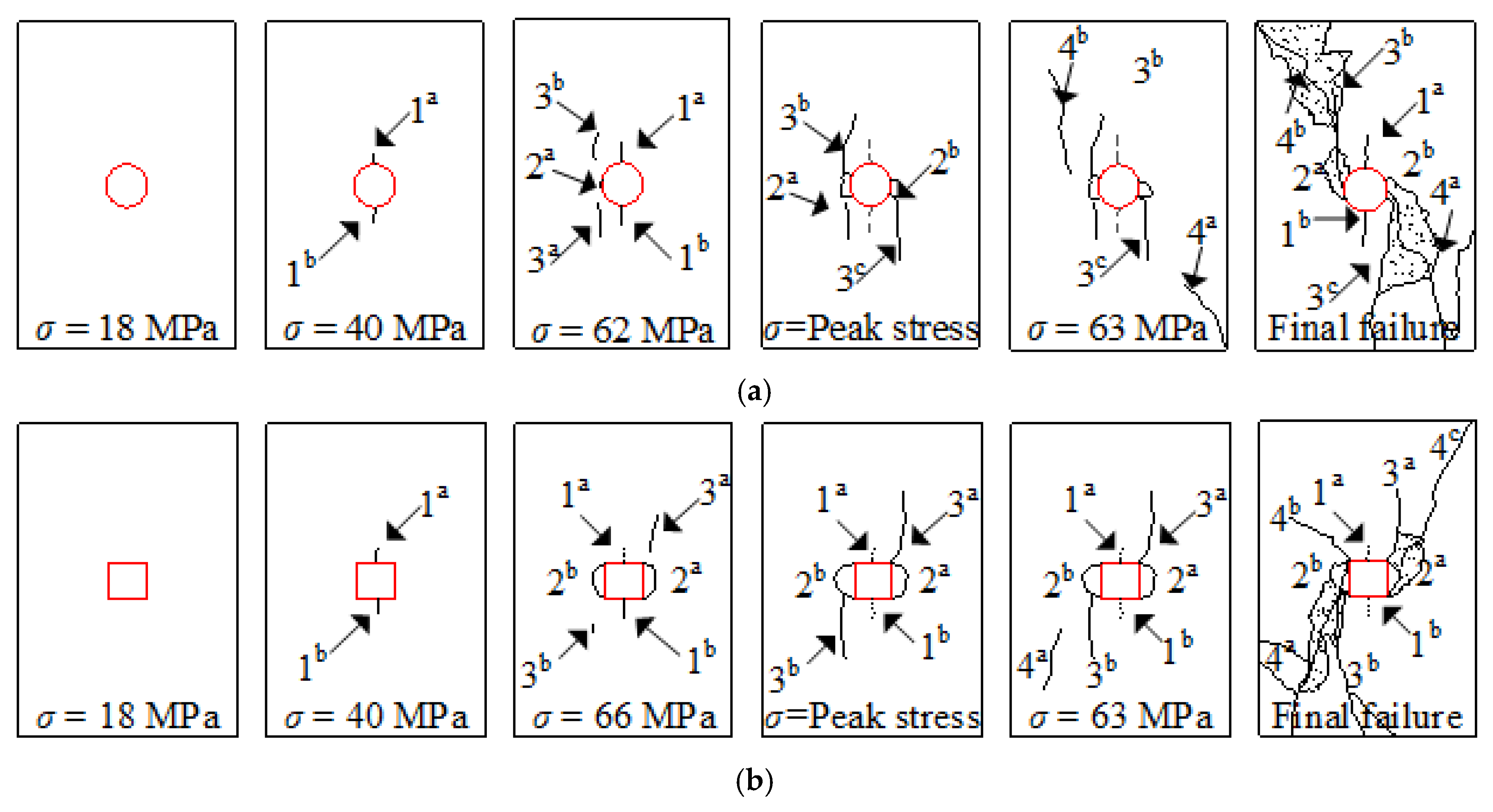
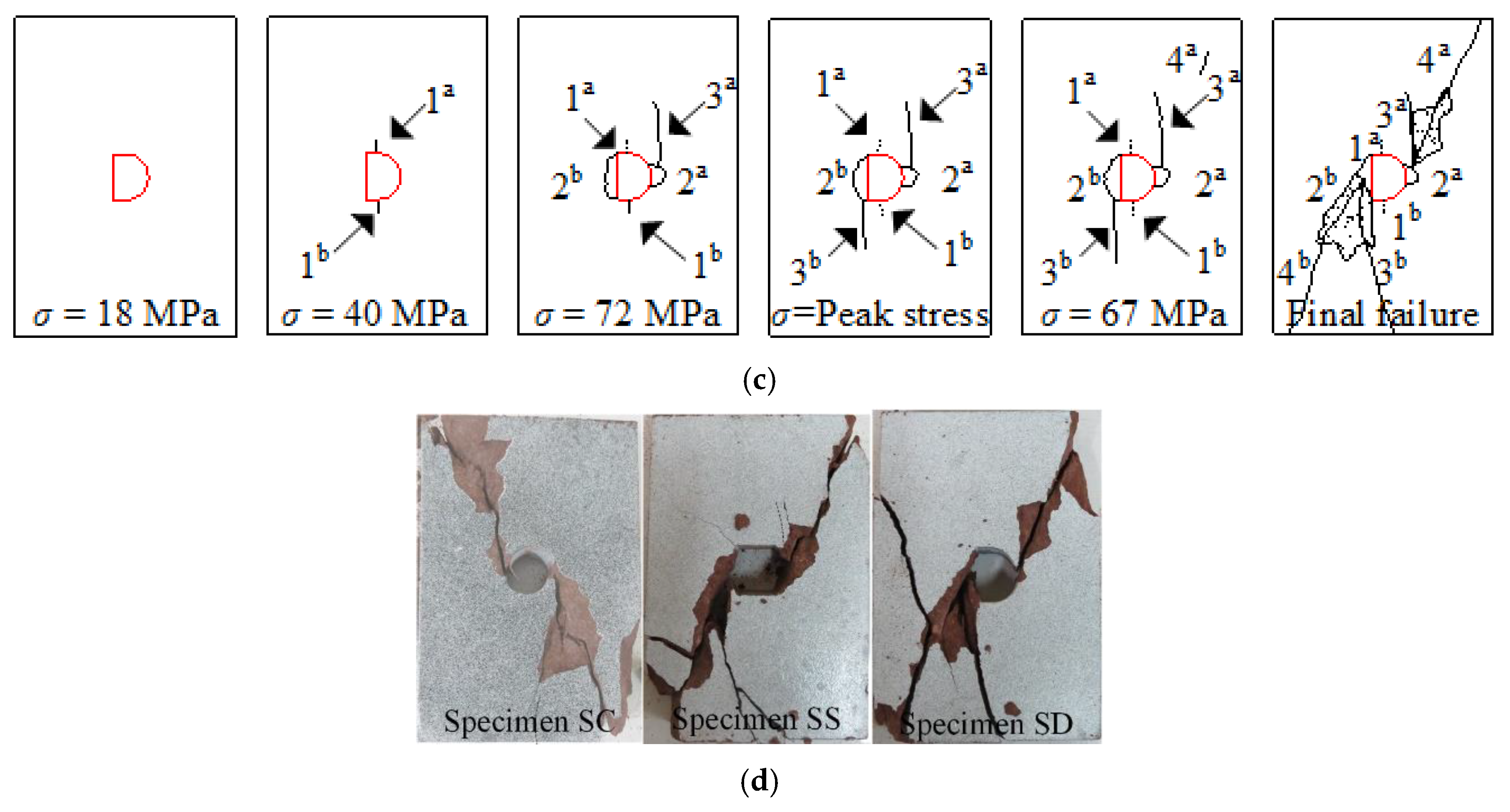
Currently, it is widely recognized that DIC (Digital Image Correlation) measurement is an advanced and promising optical test method [46]. Thus, it is extensively employed in rock mechanics experiment in recent years. Generally, the visually displayed strain localization areas by DIC technique represent the cracks formed on the speckle surface of the prismatic specimen. For details of the principle and adopted experimental apparatus, please refer to References [47,48]. Based on the DIC results [48], the crack evolution of the real rock samples with an opening subjected to uniaxial compression is sketched in Figure 13. It can be clearly seen that four identical sorts of cracks also appear around the opening in the specimen during uniaxial loading tests. In other words, the fracture process of the specimen with a prefabricated opening in uniaxial loading starts from the initial-tensile crack, via exfoliation crack and secondary-tensile crack to shear crack, and the specimen eventually suffers from shear-induced failure. The main difference between the numerical and experimental results is that the length of the tensile crack is different. The reason may be that the secondary-tensile crack will propagate to the end of the specimen when the specimen fails. Also, rock heterogeneity may have an influence on it. Besides, provided that the brittleness of the specimen is exceedingly remarkable, rock burst instead of spalling failure emerges on both sides of the opening. It should be noted that the initial-tensile cracks gradually disappear when the secondary-tensile cracks occur and propagate. The closure of the initial cracks is caused by the lateral extrusion resulting from the propagation of the secondary-tensile cracks. However, this behavior cannot be reflected in the numerical modeling. To sum up, there is good consistency in fracture evolution between the numerical and experimental investigations. This proves that the calibrated PFC model for study of brittle rock fracturing is reliable, i.e., the above optimized micro-scale parameters obtained by the proposed method are reasonable.
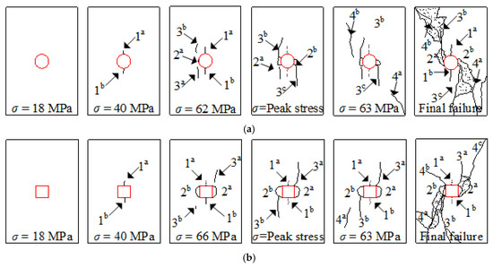
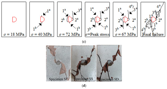
Figure 13.
Crack development around openings of different shapes under uniaxial loading obtained by experimental method: (a) sample with a circular opening, (b) sample with a square opening, (c) sample with a D-shaped opening, and (d) rock failure pattern after testing.
6. Conclusions
In this study, a coupling optimization method incorporating Box–Behnken response surface theory and desirability function optimization approach was proposed to quickly find the optimal micro-scale parameters of PFC model. After that, the calibrated model was verified by comparing the brittle fracture behavior of rock with an opening under axial loading obtained by numerical and experimental methods. Based on the results of the research, a couple of points can be concluded as follows:
- (1)
- The macroscopic mechanical properties of the parallel-bond model, including the uniaxial compressive strength, Young’s modulus, and Poisson’s ratio, are mainly controlled by three micro-scale parameters: σc, Ec, and kn/ks.
- (2)
- BB-DFO experimental design method can not only optimize multiple response variables simultaneously but also fit the nonlinear relationships between the influencing factors and the response variables. Analysis of variance indicates that the uniaxial compressive strength is extremely significantly affected by σc and kn/ks, and the interactions between σc and kn/ks and between Ec and kn/ks also have a significant influence on it. For the Young’s modulus, the effects of Ec and kn/ks as well as their interaction on it are extremely significant. In regard to the Poisson’s ratio, the impacts of Ec and kn/ks upon it are significant and extremely significant, respectively, but the effect of the interaction is not significant.
- (3)
- The optimal micro-parameters of PFC model are σc = 82.07 MPa, Ec = 20.00, and kn/ks = 2.198, and the overall desirability reaches 0.914. Correspondingly, the matched uniaxial compressive strength, Young’s modulus, and Poisson’s ratio are 102.61 MPa, 21.77 GPa, and 0.258, respectively, which are basically consistent with their experimental values (102.61 MPa, 20.78 GPa, and 0.258). Besides, the crack developments around the openings in rocks under uniaxial compression obtained by the calibrated model demonstrate good agreement with those from experimental investigation. This further proves that the micro-parameters optimized by the BB-DFO method are feasible.
Author Contributions
This research was jointly performed by H.W., B.D., G.Z., Y.C., and Y.T. Conceptualization, H.W. and B.D.; methodology, B.D.; software, Y.C. and Y. T.; validation, G.Z. and Y.T.; formal analysis, H.W.; investigation, B.D.; resources, G.Z.; data curation, Y.T and Y.C.; writing—original draft preparation, H.W.; writing—review and editing, H.W., B.D. G.Z., Y.C., and Y.T.; funding acquisition, B.D. and G.Z. All authors have read and agreed to the published version of the manuscript.
Funding
This research was funded by the National Natural Science Foundation of China (51804163 and 51774321), the China Postdoctoral Science Foundation (2018M642678), the Hunan Province Engineering Research Center of Radioactive Control Technology in Uranium Mining and Metallurgy, and Hunan Province Engineering Technology Research Center of Uranium Tailings Treatment Technology (2019YKZX2003).
Conflicts of Interest
The authors declare no conflict of interest.
References
- Belytschko, T.; Gracie, R.; Ventura, G. A review of extended/generalized finite element methods for material modeling. Model. Simul. Mater. Sci. Eng. 2009, 17, 43001. [Google Scholar] [CrossRef]
- O’Sullivan, C. Particle-Based Discrete Element Modeling: Geomechanics Perspective. Int. J. Géoméch. 2011, 11, 449–464. [Google Scholar] [CrossRef]
- Beskos, D.E. Boundary Element Methods in Dynamic Analysis. Appl. Mech. Rev. 1987, 40, 1–23. [Google Scholar] [CrossRef]
- Bobet, A.; Fakhimi, A.; Johnson, S.; Morris, J.; Tonon, F.; Yeung, M.R. Numerical Models in Discontinuous Media: Review of Advances for Rock Mechanics Applications. J. Geotech. Geoenviron. Eng. 2009, 135, 1547–1561. [Google Scholar] [CrossRef]
- Feng, F.; Chen, S.; Li, D.; Hu, S.; Huang, W.; Li, B. Analysis of fractures of a hard rock specimen via unloading of central hole with different sectional shapes. Energy Sci. Eng. 2019, 7, 2265–2286. [Google Scholar] [CrossRef]
- Cai, M.; Kaiser, P.; Morioka, H.; Minami, M.; Maejima, T.; Tasaka, Y.; Kurose, H. FLAC/PFC coupled numerical simulation of AE in large-scale underground excavations. Int. J. Rock Mech. Min. Sci. 2007, 44, 550–564. [Google Scholar] [CrossRef]
- Qiu, G.; Henke, S.; Grabe, J. Application of a Coupled Eulerian–Lagrangian approach on geomechanical problems involving large deformations. Comput. Geotech. 2011, 38, 30–39. [Google Scholar] [CrossRef]
- Banadaki, M.D.; Mohanty, B. Numerical simulation of stress wave induced fractures in rock. Int. J. Impact Eng. 2012, 40, 16–25. [Google Scholar] [CrossRef]
- Tao, M.; Zhao, H.; Li, Z.; Zhu, J. Analytical and numerical study of a circular cavity subjected to plane and cylindrical P-wave scattering. Tunn. Undergr. Space Technol. 2020, 95, 103143. [Google Scholar] [CrossRef]
- Yasitli, N.E.; Unver, B. 3Dnumerical modeling of longwall mining with top-coal caving. Int. J. Rock Mech. Min. 2005, 42, 219–235. [Google Scholar] [CrossRef]
- Feng, F.; Li, X.; Rostami, J.; Peng, D.; Li, D.; Du, K. Numerical Investigation of Hard Rock Strength and Fracturing under Polyaxial Compression Based on Mogi-Coulomb Failure Criterion. Int. J. Géoméch. 2019, 19, 04019005. [Google Scholar] [CrossRef]
- Jiang, Q.; Liu, X.; Wei, W.; Zhou, C. A new method for analyzing the stability of rock wedges. Int. J. Rock Mech. Min. Sci. 2013, 60, 413–422. [Google Scholar] [CrossRef]
- Min, K.-B.; Rutqvist, J.; Tsang, C.-F.; Jing, L. Stress-dependent permeability of fractured rock masses: A numerical study. Int. J. Rock Mech. Min. Sci. 2004, 41, 1191–1210. [Google Scholar] [CrossRef]
- Kulatilake, P.; Malama, B.; Wang, J. Physical and particle flow modeling of jointed rock block behavior under uniaxial loading. Int. J. Rock Mech. Min. Sci. 2001, 38, 641–657. [Google Scholar] [CrossRef]
- Nikolić, M.; Roje-Bonacci, T.; Ibrahimbegovic, A. Overview of the numerical methods for the modelling of rock mechanics problems. Teh. Vjesn. Tech. Gaz. 2016, 23, 627–637. [Google Scholar] [CrossRef]
- Bobet, A. Numerical methods in geomechanics. Arab. J. Sci. Eng. 2010, 35, 27–48. [Google Scholar]
- Jing, L. A review of techniques, advances and outstanding issues in numerical modelling for rock mechanics and rock engineering. Int. J. Rock Mech. Min. Sci. 2003, 40, 283–353. [Google Scholar] [CrossRef]
- Cundall, P.A. A computer model for simulating progressive large-scale movements in blocky rock systems. In Proceedings of the Symposium of International Society of Rock Mechanics, Nancy, France, 4–6 October 1971; International Society for Rock Mechanics and Rock Engineering: Salzburg, Austrian, 1971. [Google Scholar]
- Cundall, P.A.; Strack, O.D.L. A discrete numerical model for granular assemblies. Géotechnique 1979, 29, 47–65. [Google Scholar] [CrossRef]
- Cho, N.; Martin, C.; Sego, D. A clumped particle model for rock. Int. J. Rock Mech. Min. Sci. 2007, 44, 997–1010. [Google Scholar] [CrossRef]
- Wang, T.; Zhou, W.; Chen, J.; Xiao, X.; Li, Y.; Zhao, X. Simulation of hydraulic fracturing using particle flow method and application in a coal mine. Int. J. Coal Geol. 2014, 121, 1–13. [Google Scholar] [CrossRef]
- Yoon, J. Application of experimental design and optimization to PFC model calibration in uniaxial compression simulation. Int. J. Rock Mech. Min. Sci. 2007, 44, 871–889. [Google Scholar] [CrossRef]
- Hanley, K.J.; O’Sullivan, C.; Oliveira, J.; Cronin, K.; Byrne, E.P. Application of Taguchi methods to DEM calibration of bonded agglomerates. Powder Technol. 2011, 210, 230–240. [Google Scholar] [CrossRef]
- Cheung, L.; O’Sullivan, C.; Coop, M. Discrete element method simulations of analogue reservoir sandstones. Int. J. Rock Mech. Min. Sci. 2013, 63, 93–103. [Google Scholar] [CrossRef]
- Shi, C.; Yang, W.; Yang, J.; Chen, X. Calibration of micro-scaled mechanical parameters of granite based on a bonded-particle model with 2D particle flow code. Granul. Matter 2019, 21, 38. [Google Scholar] [CrossRef]
- Castro-Filgueira, U.; Alejano, L.R.; Arzúa, J.; Ivars, D.M. Sensitivity Analysis of the Micro-Parameters Used in a PFC Analysis Towards the Mechanical Properties of Rocks. Procedia Eng. 2017, 191, 488–495. [Google Scholar] [CrossRef]
- Ding, X.; Zhang, L.; Zhu, H.; Zhang, Q. Effect of Model Scale and Particle Size Distribution on PFC3D Simulation Results. Rock Mech. Rock Eng. 2013, 47, 2139–2156. [Google Scholar] [CrossRef]
- Wang, C.; Zhang, C.; Zhao, X. Application of Similitude Rules in Calibrating Microparameters of Particle Mechanics Models. KSCE J. Civ. Eng. 2018, 22, 3791–3801. [Google Scholar] [CrossRef]
- Tawadrous, A.S.; DeGagnã, D.; Pierce, M.; Ivars, D.M. Prediction of uniaxial compression PFC3D model micro-properties using artificial neural networks. Int. J. Numer. Anal. Methods Géoméch. 2009, 33, 1953–1962. [Google Scholar] [CrossRef]
- Wang, M.; Cao, P. Calibrating the Micromechanical Parameters of the PFC2D(3D) Models Using the Improved Simulated Annealing Algorithm. Math. Probl. Eng. 2017, 2017, 1–11. [Google Scholar] [CrossRef]
- Zou, Q.; Lin, B. Modeling the relationship between macro- and meso-parameters of coal using a combined optimization method. Environ. Earth Sci. 2017, 76, 479–498. [Google Scholar] [CrossRef]
- Sun, M.; Tang, H.; Hu, X.; Ge, Y.; Lu, S. Microparameter Prediction for a Triaxial Compression PFC3D Model of Rock Using Full Factorial Designs and Artificial Neural Networks. Geotech. Geol. Eng. 2013, 31, 1249–1259. [Google Scholar] [CrossRef]
- Dai, B.; Chen, Y.; Zhao, G.; Liang, W.; Wu, H. A Numerical Study on the Crack Development Behavior of Rock-Like Material Containing Two Intersecting Flaws. Mathematics 2019, 7, 1223. [Google Scholar] [CrossRef]
- Itasca Consulting Group. PFC2D (Particle Flow Code in 2 Dimensions), User’s Guide; Version 3.1; Itasca Consulting Group: Minneapolis, MN, USA, 1999. [Google Scholar]
- Yang, B.; Jiao, Y.; Lei, S. A study on the effects of microparameters on macro properties for specimens created by bonded particles. Eng. Comput. 2006, 23, 607–631. [Google Scholar] [CrossRef]
- Xu, J.; Xie, Z.; Jia, H. Simulation of mesomechanical properties of limestone using particle flow code. Rock Soil Eng. 2010, 31, 390–395. [Google Scholar]
- Zhao, G.; Dai, B.; Ma, C. Study of effects of microparameters on macroproperties for parallel bonded model. Chin. J. Rock Mech. Eng. 2012, 31, 1491–1498. [Google Scholar]
- Box, G.E.P.; Wilson, K.B. On the Experimental Attainment of Optimum Conditions. J. R. Stat. Soc. Ser. B Stat. Methodol. 1951, 13, 1–38. [Google Scholar] [CrossRef]
- Candioti, L.V.; De Zan, M.M.; Cámara, M.S.; Goicoechea, H.C. Experimental design and multiple response optimization. Using the desirability function in analytical methods development. Talanta 2014, 124, 123–138. [Google Scholar] [CrossRef]
- Cao, W.; Shi, J.; Durucan, S.; Korre, A.; Jamnikar, S. Numerical modelling of anomalous microseismicity influenced by lithological heterogeneity in longwall top coal caving mining. Int. J. Coal Geol. 2019, 216, 103305. [Google Scholar] [CrossRef]
- Zhou, Z.; Wang, H.; Cai, X.; Chen, L.; Cheng, R. Damage Evolution and Failure Behavior of Post-Mainshock Damaged Rocks under Aftershock Effects. Energies 2019, 12, 4429. [Google Scholar] [CrossRef]
- Martin, C.; Christiansson, R. Estimating the potential for spalling around a deep nuclear waste repository in crystalline rock. Int. J. Rock Mech. Min. Sci. 2009, 46, 219–228. [Google Scholar] [CrossRef]
- Afraei, S.; Shahriar, K.; Madani, S.H. Developing intelligent classification models for rock burst prediction after recognizing significant predictor variables, Section 1: Literature review and data preprocessing procedure. Tunn. Undergr. Space Technol. 2019, 83, 324–353. [Google Scholar] [CrossRef]
- Liu, B.; Malekian, R.; Xu, J. Groundwater Mixing Process Identification in Deep Mines Based on Hydrogeochemical Property Analysis. Appl. Sci. 2016, 7, 42. [Google Scholar] [CrossRef]
- Ko, T.Y.; Lee, S.S. Experimental Study on Stress Corrosion Index Governing Time-Dependent Degradation of Rock Strength. Appl. Sci. 2020, 10, 2175. [Google Scholar] [CrossRef]
- Schreier, H.; Orteu, J.-J.; Sutton, M. Image Correlation for Shape, Motion and Deformation Measurements: Basic Concepts, Theory and Applications; Springer Publishing Company, Incorporated: New York, NY, USA, 2009. [Google Scholar]
- Wu, H.; Zhao, G.; Liang, W. Investigation of cracking behaviour and mechanism of sandstone specimens with a hole under compression. Int. J. Mech. Sci. 2019, 163, 105084. [Google Scholar] [CrossRef]
- Wu, H.; Zhao, G.; Liang, W. Mechanical properties and fracture characteristics of pre-holed rocks subjected to uniaxial loading: A comparative analysis of five hole shapes. Theor. Appl. Fract. Mech. 2020, 105, 102433. [Google Scholar] [CrossRef]
© 2020 by the authors. Licensee MDPI, Basel, Switzerland. This article is an open access article distributed under the terms and conditions of the Creative Commons Attribution (CC BY) license (http://creativecommons.org/licenses/by/4.0/).

