Abstract
Monthly rainfall forecasts can be translated into monthly runoff predictions that could support water resources planning and management activities. Therefore, development of monthly rainfall forecasting models in reservoir watersheds is essential for generating future rainfall amounts as an input to a water-resources-system simulation model to predict water shortage conditions. This research aims to examine the reliability of linking a data preprocessing method (singular spectrum analysis, SSA) with machine learning, least-squares support vector regression (LS-SVR), and random forest (RF), for monthly rainfall forecasting in two reservoir watersheds (Deji and Shihmen reservoir watersheds) located in Taiwan. Merging SSA with LS-SVR and RF, the hybrid models (SSA-LSSVR and SSA-RF) were developed and compared with the standard models (LS-SVR and RF). The proposed models were calibrated and validated using the watersheds’ observed areal monthly rainfalls separated into 70 percent of data for calibration and 30 percent of data for validation. Model performances were evaluated using two accuracy measures, root mean square error (RMSE) and Nash–Sutcliffe efficiency (NSE). Results show that the hybrid models could efficiently forecast monthly rainfalls. Nonetheless, the performances of the hybrid models vary in both watersheds which suggests that prior knowledge about the watershed’s hydrological behavior would be helpful to implement the appropriate model. Overall, the hybrid models significantly surpass the standard models for the two studied watersheds, which indicates that the proposed models are a prudent modeling approach that could be employed in the current research regions for monthly rainfall forecasting.
1. Introduction
In hydrological research, timely rainfall forecasts are of major concern, and can be used to deliver valuable data for agrarian development, controlling of water resources, and application of crop insurance [1,2]. Additionally, accurately forecast rainfalls can be used for reservoir operation and flooding prevention [3,4]. However, the spatial and temporal rainfall distribution has substantial consequences on the water availability on land and thus on agrarian operations. Considering that agricultural operations and crop production rely on the rainfall distribution, monthly rainfall forecasting is critical for agricultural scheduling and flood control. However, accurate forecasting of monthly rainfall remains a major challenge among hydrologists. Monthly rainfall forecasting with an appropriate method is an essential requirement to support water resources management [5,6]. Therefore, monthly rainfall forecasting is widely applicable in the field of hydrology [7,8]. For example, in Taiwan, due to industrial expansion and population growth, the demand for water has risen, and the hydrologic variability has increased, possibly because of the impact of climate change [3]. The forecasting of monthly precipitation is then very critical in Taiwan.
Several techniques for forecasting time series have been developed on a global scale [9,10,11,12,13,14]. Artificial intelligence or machine intelligence (MI) and stochastic models based on data extraction techniques are the most widely used time series modelling approaches for hydrological forecasting.
However, MI has been paid more attention in hydrological forecasting, mainly because stochastic models consider that the time series is stationary and have a limited ability to capture highly nonlinear characteristics of rainfall series [15,16]. Hydrological time series in actual use are typically non-stationary and non-linear, so predicting maximum values is extremely difficult [17]. Ref [18] states that the forecasts by artificial neural networks (ANNs) are more precise than traditional statistical and numerical methods. Ref [19] shows that by deploying suitable contemporary mathematical methods such as ANNs, superior seasonal rainfall forecasts can be accomplished. The problems of linear predictive models paved the way for the enormous use of models based on MI. For these reasons, the current study justifies the need to apply machine intelligence.
Methodologies based on data-driven, MI systems (MI) have been extensively and successfully applied in many fields [20]. MI has become a common inductive strategy in rainfall forecasting owing to its extremely nonlinear, flexible, and data-driven model training without first understanding catchment and flow processes [21]. Despite the popularity of MI models for time series forecasting, they are not an efficient tool to forecast long-term rainfall [22]. The most extensively used MI-based models for rainfall forecasting include support vector machine, genetic programming, ANN, and fuzzy logic [23,24]. Hybrid approaches for addressing different hydrological problems have been favored by water resources scientists.
Recently, hybrid MI concepts have been used for effective modelling and forecasting of rainfall [25]. Ref [26] proposes a hybrid system, the Adaptive Neuro-Fuzzy Inference System (ANFIS), to improve long-term rainfall forecasting. The findings demonstrate that the ANFIS is capable of capturing the rainfall data’s dynamic behavior and generates satisfactory outcomes. Ref [27] merged ANNs with wavelet analysis (WA) to forecast rainfalls at an Iranian meteorological station and the hybrid model was contrasted with ANFIS. The findings demonstrate that the hybrid model coupling ANNs with WA is more efficient than the ANFIS and is suitable for rainfall forecasting. Ref [5] compares multiple artificial intelligence techniques to forecast the daily and monthly average rainfall in Fukuoka city, Japan. They proposed a hybrid multi-model and contrasted it to its component models. The results show that, for the daily rainfall sequence, the hybrid technique generates a more precise prediction than the single models. Ref [22] developed a one-month WA-ANN coupling model for rainfall forecasting in Iran and demonstrated that the coupled model can equally forecast short- and long-term rainfall occurrences. Ref [28] proposed gene expression programming (GEP) and hybrid WA-GEP models for daily sequence forecasting at two weather stations in Turkey. Results show that the WA-GEP model considerably increases the effectiveness of the results of the single GEP. Ref [29] used dyadic wavelets and neural networks as a means of predicting drought in the Conchos Basin, Mexico, and the findings show that the joint system significantly increased the capacity of neural networks to predict drought.
Least-square support vector regression (LS-SVR) has recently received considerable attention in various forecasting problems [30,31,32]. In the current study, LS-SVR was chosen because it is computationally more appealing than the traditional support vector regression (SVR). Based on the use of quadratic programming with nonlinear equations, the standard SVR has computational difficulties to decide the optimal solution [33,34,35,36,37]. The hybrid simulation approach based on LS-SVR as a forecasting model delivers excellent outcomes. For example, [38] suggested singular spectrum analysis (SSA) and the SVR for runoff and rainfall forecasting. The findings show a significant improvement in model efficiency compared to the initial SVR model. Ref [39] developed a WA-SVR hybrid flow forecasting technique. The WA-LSSVR is compared to the LS-SVR, wavelet regression (WR) and linear regression (LR). The results show that the WA-LSSVR is more accurate in river flow forecasting than the aforementioned models. Ref [22] developed an SVR and firefly algorithm (SVR-FFA) at two rainfall stations for one-month rainfall forecasting. The findings demonstrate that the hybrid model is better able to capture the nonlinear features of monthly rainfall than the SVR and Multigene Genetic Programming models. Ref [40] developed a downscaling method by LS-SVR for improving the downscaling of extreme rainfall. Ref [41] used LS-SVR to forecast the reservoir inflows of Demirkopru Dam in Turkey. The findings promote LS-SVR efficiency. Ref [42] forecast multistep-ahead flow by means of LS-SVR, with the everyday river flow changes modelled prior to forecasting. Ref [43] used LS-SVR to calibrate parameters and to develop models. The study shows that the SVR approach is superior to the Box–Jenkins approach. The study concludes that the explanation for SVR’s good performance lies in the non-linear characteristic of the captured and used SVR space.
More recently, interest in applications of random forest (RF) has extended to a number of areas [44,45,46]. However, there are only few applications of RF in hydrology. Ref [40] applied RF and LS-SVR to boost downscaling of intense precipitation. Ref [47] used RF for rainfall forecasting at Besut station on the eastern coast of the Malaysian Peninsula. Ref [48] carried out a comprehensive literature review to compare various approaches of machine learning, including SVR and RF. Ref [49] argues that RF offers a good alternative to SVR and has often performed better than SVR. Ref [50] developed an RF-based evaluation model for evaluating regional flood hazards, and [51] suggested a RF-based drought forecast to predict the monthly standardized precipitation index (SPI) time series. Ref [52] forecasted the start of winter rain by RF in Australia. Ref [53] applied RF in Vietnam to forecast the incoming flood of the Hoa Binh reservoir. Ref [54] proposed RF for daily and monthly rainfall forecasting. Ref [55] compared ANN, SVR, and RF performances in general flood applications and RF delivered the best output. Nevertheless, there is no study of RF-based models with a data preprocessing technique for monthly rainfall forecasts, which prompts this current study to introduce a hybrid model coupling RF with a data preprocessing technique.
Today, data preprocessing approaches have been applied to break down observed data into subseries so as to boost the accuracy of time series forecasting. Efficient forecast outcomes can be enhanced with independent modeling of subseries. The most extensively applied approaches of preprocessing data can be found in wavelet transformation [56], singular spectrum analysis (SSA) [57], ensemble empirical mode decomposition [58], and principal component analysis [59].
SSA has been applied to many different areas such as medical engineering [60], economics [61] and hydrology [62]. The SSA strategy comprises two phases: decomposition and reconstruction. In this study, only decomposition was implemented. Decomposition into different principle components (PCs) of the initial time series including trend patterns, oscillating components and noise [57]. It is used to conduct a spectrum analysis of the input data, remove high-frequency components, and invert the remaining components to produce a ‘filter’ time series. In SSA, different parts of a time series can be extracted [63,64]. For data pretreatment and modeling, SSA has shown that it is a successful algorithm [65,66]. Ref [17] introduced SSA in order to forecast rainfall at an Indian weather station. The results demonstrate that the SSA technique can separate the different components of the time series efficiently and allow forecasting day-to-day precipitation for a long period, such as one year in a single cycle, with fair precision. Ref [67] compare wavelet analysis with SSA. The results indicate that SSA performs better than WA. Ref [68] propose a hybrid model of an SSA adaptive noise reduction algorithm and a traditional feed-forward neural network forecasting, with the goal of significantly improving short- and long-duration time series forecasting. The findings indicate that the coupled model has superior performance as compared with the forecasts provided directly on raw data by the same network and is therefore well suited for forecasting short and noisy time series with the intrinsic deterministic method of data output. Ref [69] used SSA for decomposing and reconstructing water consumption with six climate variables so as to build a time series for seasonal forecasting. The SSA model is an efficient tool that can split the original time series down into a quantity of separate components, including trend patterns, oscillating components, and noise. Ref [62] applied SSA to annual precipitation, monthly runoff, and hourly water temperature time series to evaluate its capacity and forecasting ability to distinguish significant information from those series. The research concludes that the SSA has the ability to obtain and provide excellent predictions for significant hydrological time series components with distinctive uneven behaviors, such as precipitation and runoff series. Ref [70] introduced SSA to extract a trend. The study showed that SSA is an attractive trend extraction technique, since it needs no model description of time series and trend, extracts noisy time series trends with uncertain oscillations in time series, and is sensitive to outliers. The aforementioned literature shows the significance of using a suitable data preprocessing method (SSA) to raw input signals to supply high quality data before being implemented as a model input. Although a large number of previous studies have been conducted to explore the advantage of coupled data preprocessing and machine leaning, to the best of our knowledge, this is the first time that SSA coupled with LSSVM and RF has been used for monthly rainfall forecasting. Subsequently, these two coupled models (i.e., SSA-LSSVM and SSA-RF) are compared to find a better model for each reservoir watershed.
There is convincing evidence that the hybrid modeling approach based on LS-SVR and RF is reliable and that the SSA produces superior outputs. Thus, for improving the forecasting performance of the standard models, the data preprocessing technique is adopted in the current study. The primary objectives are as follows:
- Linking SSA with machine learning techniques (i.e., LS-SVR and RF) to construct hybrid models (SSA-LSSVR and SSA-RF) for monthly rainfall forecasting in two reservoir watersheds of Taiwan where the hybrid models have not been applied before.
- Comparison between the hybrid models (i.e., SSA-LSSVR and SSA-RF) and the standard models (i.e., LS-SVR and RF) to validate the efficiency of the data preprocessing technique.
The remainder of this paper is arranged as follows. Section 2 (“Study Sites and Data collection’’) summarizes the study sites and the data collection. Section 3 (“Methodology”) briefly describes the machine learning techniques (LS-SVR and RF), data preprocessing technique (SSA), coupling of SSA with LS-SVR and RF, and measurement of model performance. Section 4 (“Results and Discussion”) shows the results of the proposed models for monthly rainfall forecasting, and elaborates and discusses the findings of the current study. Section 5 (“Conclusions”) gives the conclusions and considers the need for future work.
2. Study Sites and Data Collection
Taiwan is located in the Western Pacific Ocean. The East Asian Monsoon characterizes its climate. The main sources of rainfall are heavy rainfall systems (Mei-Yu front) and typhoon events. The average rainfall for Taiwan is 2510 mm per year, spatially and temporally unequally distributed. About 70 percent of the annual rainfall occurs in the rainy season (May–October), and the dry season occurs from November to April.
This present study selected the Shihmen and Deji reservoir watersheds as the study areas, as shown in Figure 1. The study areas were chosen as the research interest for rainfall forecasting because they are critical to water resources in Taiwan. The watershed area of Shihmen reservoir is situated in the Danshuei river basin, in the north of Taiwan. The storage capacity in this reservoir is around 309 million m3. The watershed’s area is 763 km2 and the reservoir’s elevation is 250 m above sea level. The annual average rainfall is about 2250 mm. In 1964, Shihmen reservoir was constructed as a multipurpose water supply storage tank for water irrigation and was used to produce hydroelectricity, prevent flooding, and for recreation [71]. Deji reservoir is situated in the middle of northern Taiwan. It has a capacity of about 266 million m3. The watershed covers an area of 1411 m above sea level. The annual average rainfall is about 2450 mm. Like Shihmen reservoir, Deji reservoir has been used since 1974 to supply municipal water, to produce hydropower, for recreation, and to prevent flooding.
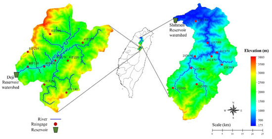
Figure 1.
Deji and Shihmen Reservoir watersheds.
Data were collected from Taiwan Water Resource Bureau, which includes the monthly rainfall data during 1958–2018 for each rain gauge in the Shihmen watershed and during 1981–2017 for each rain gauge in the Deji Reservoir watershed. For each reservoir watershed, the first 70% of the entire data collection was used for training, and the remaining 30% for validation. Table 1 and Table 2 present geographical information on the two studied watersheds. The areal monthly rainfalls for each reservoir watershed were calculated using the Thiessen polygon method to calculate areas in relationship to the rain gauges and thereby compute the average amount of rainfall (areal rainfall) that fell in the watershed, which was then used for constructing the rainfall forecasting models in the present study.

Table 1.
Geographic information on the rain gages in the Deji Reservoir watersheds.
Table 2.
Geographic information on the rain gages in the Shihmen Reservoir watershed.
To understand the characteristics of the monthly rainfall series in Deji and Shihmen Reservoir watersheds, the descriptive statistics were used for exploring their rainfall characteristics. The statistical behavior of any hydrological series can be described based on certain parameters such as mean, standard deviation, kurtosis, skewness, and coefficient of variation. In the present study, the mean, standard deviation, skewness, and kurtosis are used to describe the variability of monthly rainfall. Using the observed data, the descriptive statistics of rainfall data were estimated. Table 3 shows the statistical parameters of the monthly rainfall series for the two reservoir watersheds. The standard deviation value indicates that the precipitation pattern varies greatly. The skewness values show that rainfall patterns do not comply with a normal distribution. The skewness and kurtosis indicate differences in their statistical distribution.
Table 3.
Statistical parameters of monthly rainfall series for the two Reservoir watersheds.
3. Methodologies
3.1. Least-Squares Support Vector Machine
The least-squares support vector machine (LS-SVM), a new type of SVM, comprises a sequence of similar supervised learning techniques that analyze data and identify patterns. Based on the constraints of equality rather than inequality, the LS-SVM technique is employed for classification and regression [72]. Instead of resolving the convex quadratic programming problem, LS-SVM solutions are reached by resolving a series of linear equations. This alteration decreases the computational complexity and makes the LS-SVM more attractive. In addition, the model has the benefits of simplifying the problem and solution finding without losing precision [73,74]. More detailed information about LS-SVM is available from [75]. The LS-SVM technique has been applied to a variety of fields such as text classification [23,76], image processing [77,78], and time series forecasting [79,80]. In this analysis, the LS-SVR is applied to forecast monthly rainfall. In the following section, we briefly present the basic theory on LS-SVR in time series forecasting.
Considering a training set as input data xi and output yi, the regression function that links the input vector to the output can be defined as [81]:
where the nonlinear mapping maps the input data into a higher-dimensional feature space. Transforming the regression problem in Equation (1) into a constrained quadratic optimization problem, by minimizing the cost variable, w and b can be estimated. In the structural minimization principle, the regression problem can be formulated as:
subject to the following constraints:
where denotes the penalty term and ei is the training error for xi. In order to solve the optimization problem, the solution for optimizing the LS-SVM is to create a Lagrangian function as follows:
whereare the Lagrange multipliers (support values).
Under the state of the Karush condition [82], we can partially differentiate the solution of Equation (4) to obtain w, b, e and alpha, respectively, as:
ei and w elimination would generate a linear process rather than a quadratic problem of programming:
where
By constructing the kernel function, Mercer’s theorem can be fulfilled (a detailed explanation of the Mercer’s condition can be found in [83]). Next, the LS-SVM method is implemented for estimating the function:
Within LS-SVM, there are many possible choices for the kernel function, such as sigmoid kernel, polynomial kernel, linear kernel, and radial bias function (RBF). The latter has fewer parameters and needs to be adjusted for practical problems. In this study, we apply the Gaussian RBF kernel [84,85] followed by Equation (8):
In the formula stated above two parameters need to be chosen: the penalty term (𝛾) and the kernel bandwidth sigma (σ). In this work, we used the LS-SVR implementation from the MATLAB toolbox LSSVMLAB.
3.2. Random Forest
Random forest (RF) is one of the most powerful machine learning models for predictive analysis, comprising of a range or group of simple trees. RF is an enhancement of the decision tree model based on the method of bagging (bootstrapping + aggregating). The bagging method may constitute the overfitting problem of computer models. In bagging, multiple stochastic error scenarios are performed by choosing training sets individually and randomly from the total historical observation set; aggregating the forecast of each individual trained model is accomplished by taking its arithmetic mean value. The decision tree model is chosen as the individual model of forecast in the RF-based model. In addition to forecasting, RF can also assess the significance of explaining variables to the forecast according to the simple rule, “the more relevant the explanatory variable, the more important the effect on the forecast” in order to use the RF-based model for the selection of variables. In bootstrap sampling, the total observations are divided into two groups for each individual model: in-bag subset (i.e., training subset) and out-of-bag subset. The out-of-bag subsets may be used to determine the significance of each explanatory variable: (1) randomizing the values for one chosen explanatory variable in the out-of-bag subset; (2) using the randomized out-of-bag subset and the original sample to make new predictions; (3) testing the significance of the chosen explanatory variable by increasing the mean square error of the new forecast. A detailed description of RF can be found in [86,87,88]. The current study employs the random forest package [88].
3.3. Singular Spectrum Analysis
SSA presents an effective approach to time series analysis in many areas of scientific research [89]. The SSA approach is particularly important when time series are decomposed into major components like trend patterns, oscillations, and noise [64]. A major benefit of the SSA approach is that it is nonparametric, meaning it can be tailored to the underlying data set and deny the need for an a priori model. For this reason, the SSA technique is considered a model-free method. According to [90], two supplementary stages are involved in the SSA method: decomposition and reconstruction. The theoretical development of SSA is as follows.
Decomposition
The process of decomposition comprises two steps: embedding and singular value decomposition (SVD). This decomposition is the main result of the SSA algorithm. Decomposition is important when each restored subsection can be categorized as either a trend pattern, or as an oscillation or aspect of noise.
Step 1: Embedding
The embedding step is the initial step in the SSA algorithm. This method converts the observed time series to a multi-dimensional vector sequence.
The embedding technique maps the original time series by shaping lagged vectors of the series f as:
In Equation (9) we notice that has the same elements on the anti-diagonals. This type of matrix is called a Hankel matrix.
According to [90], the size of the window L should be sufficiently large, but less than half of the time series. Larger values of L allow longer period oscillations to be detected, but a too-high value of L may require a large number of eigentriples and skip some essential major components with high contributions. Ref [62] selected window length L from experience, [91] repeatedly tried with varying window length, and another study [92] used proportional data length, such as . In the present study, the method of proportional data length proposed by [92] is adopted.
Step 2: Singular Value Decomposition (SVD)
The SVD of the trajectory matrix is the primary component of the decomposition process. From matrix, define the covariance matrix. The SVD of provides a set of eigenvalues in descending order of magnitude and the corresponding eigenvectors The SVD of the trajectory matrix can then be formulated as:
where and (equivalent to the ith column of ). The matrices have rank 1; thus, they are elementary matrices. The collection denotes the ith eigentriple.
3.4. Coupling SSA with Machine Learning (LS-SVR and RF)
The values of monthly rainfall were standardized by their respective means and standard deviations prior to training the standard models (LS-SVR and RF). To train the standard models, the standardized rainfall values were then used. As mentioned in Section 3.1, two parameters, the penalty term (γ) and the kernel width (σ), should be selected in the calibration process of the LS-SVR model. The grid search technique is utilized for optimizing parameters during the calibrating period of the LS-SVR model. The grid search technique is capable of producing an optimum parameter set and can overcome the problems of over-fitting of the model by means of the cross-validation procedure.
RF has two parameters, the number of variables (mtry) and the number of trees (ntree), which need to be determined. Ref [93] found that (mtry) would usually produce near-optimum results, so the value of mtry was selected by trial and error using the value around (value of M is 4). The range of ntree from 0 to 2000 was used to search the best value. However, no substantial change was achieved compared to the default value for ntree of 500. Hence, the value of 500 for ntree was adopted in this current study.
The areal monthly rainfalls in Deji Reservoir watershed from 1981–2017 and in Shihmen Reservoir watershed from 1958–2018 were used. In Deji Reservoir watershed, the first 25 years of rainfall data were applied for training and the remaining 10 years of rainfall data were used for testing, whereas in Shihmen Reservoir watershed, the first 41 years of rainfall data were used for training and the remaining 18 years of rainfall data were used for testing. The areal monthly rainfall forecasting for each reservoir watershed was implemented using the forecasting models (i.e., LS-SVR and RF). The collection of appropriate input data sets is a major concern for LS-SVR and RF modeling. Different combination of antecedent values of the rainfall data were considered as inputs (i.e., (1) R(t); (2) R(t), R(t-1); (3) R(t), R(t-1), R(t-2)). The output is rainfall times series data to be forecasted with 1-, 2-, and 3- month lead-time (i.e., R(t+1), R(t+2), and R(t+3)).
The hybrid models (i.e., SSA-LSSVR and SSA–RF) were obtained by combining two different methods. In view of the SSA’s dominance, the hybrid models are designed to improve forecasting performance and reliability. The results of the standard and hybrid models are compared to assess the model performance in rainfall forecasting in different study catchments.
The subsequent steps give a summary of the methodological processes for the model:
- Initially, the time series of rainfall data was decomposed into several principal components (PCs) using SSA.
- The relevant principal components are calculated on the basis of the trend or period of each series, and a new series for each variable is constituted by adding up the primary components to be defined. The new series was used to construct model input.
- LS-SVR and RF models are applied to every component of the reconstruction so that the architecture of LS-SVR and RF is different for each component of the reconstruction.
- Finally, LS-SVR and RF models are fed with the new series to forecast the future rainfalls for 1-, 2-, and 3- month lead-time. This is the principal idea of coupling SSA with machine learning techniques (LS-SVR and RF), as illustrated in Figure 2.
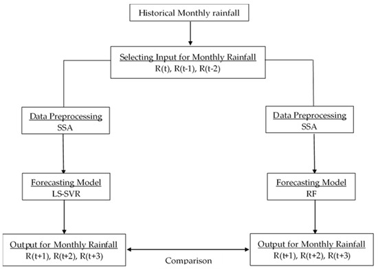 Figure 2. Structure of the hybrid model (i.e., SSA-LSSVR, and SSA–RF).
3.5. Forecast Verification
The performances of the forecasting models are analyzed using the two criteria, root mean square error (RMSE) and the Nash–Sutcliffe model efficiency coefficient (NSE), for the calibration and validation periods. The definitions of the different criteria are presented below:
where and are the observed and estimated values, respectively. Smaller values of RMSE suggest higher accuracy.
An NSE of 0.75–1.0 corresponds to a “very good” performance, 0.65–0.75 to a “good” performance, and 0.5–0.65 to a “reasonable performance”, while values below 0.5 reflect unsatisfactory performance [94]. In essence, the closer NSE is to 1, the more accurate is the forecast.
4. Results and Discussion
The current study constructed the monthly rainfall forecasting models for 1-, 2-, and 3-month lead-time for two reservoir watersheds (i.e., Deji and Shihmen) in different regions of Taiwan. The standard models (i.e., LS-SVR and RF) and the hybrid models (i.e., SSA-LSSVR and SSA-RF) have comparable processes for the data modeling. The difference is that the standard models used the raw data as model input, whereas the hybrid models used the decomposed input data generated by SSA instead of raw data. Table 4 presents the forecasting performances for 1-, 2-, and 3- month lead-time for the standard and hybrid models during the validation period by the criteria of RMSE and NSE.
Table 4.
Forecasting performances of the LS-SVR and SSA-LSSVR models during the validation period.
As observed from Table 4, it is found that RMSE and NSE exhibit very poor values for the standard models using original data when compared to the hybrid models using data generated by SSA. There is also evidence that the standard models have been poorly validated for all three lead-times (i.e., 1-, 2-, and 3- month lead-time). Using only the original data as input for rainfall forecasting seems less efficient than using the data generated by SSA. The LS-SVR’s output is noise-sensitive and may not be effective when the level of noise is high. Therefore, the LS-SVR coupling with the SSA filtering the raw rainfall data will reduce the noise effects. Furthermore, the trained LS-SVR in conjunction with the SSA thus paid greater attention to the noise sensitivity, increasing the overall forecasting performance of the hybrid model. Ref [68] suggested that the coupled model (the SSA with predictive model) has superior performance as compared to those directly using the raw data and is therefore well suited for forecasting noisy time series.
Figure 3 and Figure 4 illustrate the time-series graphs of the observed and 1-month lead-time forecasted rainfalls by the standard models during the validation process for Deji and Shihmen Reservoir watersheds respectively. From the figures, we find that the forecasted values from the hybrid models are closer to the observed values than the values forecasted by the standard models. The scatterplots of observed vs. values forecasted by the standard models (LS-SVR and RF) and the hybrid models (SSA-LSSVR and SSA-RF) in Deji and Shihmen Reservoir watersheds are also illustrated in Figure 5 and Figure 6 for 1-,2-, and 3-month lead-time forecasts, respectively. The rainfalls forecasted by the hybrid models were found to be very closely limited to the line of equality, whereas the rainfalls forecasted by the standard models are not close to the line of equality. This also reveals that the standard models without a data preprocessing technique are not efficient to forecast rainfalls and the hybrid models are able to approximate different rainfall properties much better than the standard models.
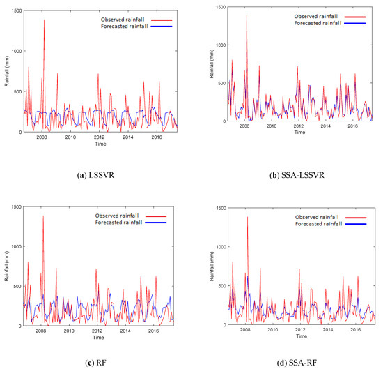
Figure 3.
Time-series graphs comparing the observed and forecasted rainfalls by the (a) LS-SVR, (b) SSA-LSSVR, (c) RF, and (d) SSA-RF models during the validation period for Deji Reservoir watershed 1-month lead time.
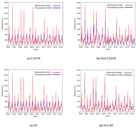
Figure 4.
Time-series graphs comparing the observed and forecasted rainfalls by the (a) LS-SVR, (b) SSA-LSSVR, (c) RF, and (d) SSA-RF models for Shihmen Reservoir watershed 1-month lead time.
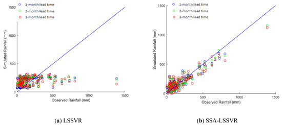
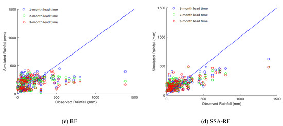
Figure 5.
Scatterplots of the observed vs. forecasted rainfalls by the (a) LS-SVR, (b) SSA-LSSVR, (c) RF, and (d) SSA-RF models during the validation period for Deji reservoir watershed 1-,2-, and 3-month lead time.
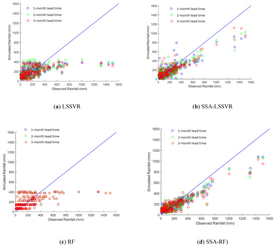
Figure 6.
Scatterplots of the observed vs. forecasted rainfalls by the (a) LS-SVR, (b) SSA-LSSVR, (c) RF, and (d) SSA-RF models during the validation period for Shihmen reservoir watershed 1-,2-, and 3-month lead time.
Moreover, the performances of the hybrid models (SSA-LSSVR and SSA-RF) vary in both reservoir watersheds. For example, the SSA-LSSVR forecasts better than the SSA-RF in Deji reservoir watershed for all three lead-times. NSE values above 0.75 may characteristically be considered as a “very good” performance [94]. From Table 4, it is clear that all the values of NSE by the SSA-LSSVR in the Deji Reservoir watershed are greater than 0.75 and the values of the RMSE of the SSA-LSSVR are lower than the values of SSA-RF. Hence, the SSA-LSSVR outperforms the SSA-RF in the Deji Reservoir watershed. In the Shihmen Reservoir watershed, it can be seen that the NSE values of SSA-RF for each of the three lead-times belong to the “very good” performance class, whereas the NSE values of SSA-LSSVR indicate “good” performance between 0.65 and 0.75 for all three lead-times. Similarly, the RMSE values of SSA-RF are lower than the values of SSA-LSSVR for 1- and 2-month lead-time, while the RMSE value of the SSA-RF is close to the value of SSA-LSSVR for 3- month lead-time. From this analysis, it is clear that the RF-SSA is superior to the SSA-LSSVR in Shihmen Reservoir watershed. Figure 5 and Figure 6 illustrate the scatterplots of the observed vs. forecasted rainfalls for (a) SSA-LSSVR, (b) SSA-RF for Deji Reservoir watershed, and 6(c) SSA-LSSVR, 6(d) SSA-RF for Shihmen Reservoir watershed during the validation for 1-, 2-, and 3-month lead-time. In Figure 5b,d, it can be seen that the SSA-LSSVR forecasts are better than the SSA-RF forecasts in Deji reservoir watershed for 1-,2-, and 3-month lead-time. From Figure 6b,d, the SSA-LSSVR and SSA-RF perform similarly in Shihmen Reservoir watershed for 3-month lead-time.
The above results show that the SSA-LSSVR outperforms the SSA-RF in Deji Reservoir watershed, whereas the SSA-RF is superior to the SSA-LSSVR in Shihmen Reservoir watershed, which may be attributed to the different rainfall characteristics of the catchment. The catchment characteristics are an important feature of all models for hydrological simulation and prediction. The performance of simulation and prediction techniques for single hydrometric stations differ according to their watershed climate zone and characteristics, and the climate conditions in different watersheds will significantly affect the effectiveness of different forecasting techniques [95]. In some cases, the behavior of the watersheds is more sensitive to the effects of rainfall patterns, so some models would perform better than others [96].
In general, given the aforementioned differences in model performances, our findings support the view that the hybrid models are more efficient for monthly rainfall forecasting than the standard models. Furthermore, the performances of the two hybrid models (SSA-LSSVR and SSA-RF) vary in both reservoir watersheds, which might result from different hydrological behaviors (e.g., rainfall patterns). Having a prior knowledge of the rainfall characteristics (standard deviation, skewness, and kurtosis) of the studied watershed would be helpful to apply the suitable model. However, to be able to make a thorough conclusion, more study cases should be investigated in future work. On the basis of our current findings, only a general assumption can be drawn that if the standard deviation, skewness, and kurtosis values are small then SSA-LSSVR may perform better as seen in Table 3; otherwise, SSA-RF should be preferred. Thus, the current study preliminarily investigated the characteristics of the monthly rainfall series for the two reservoir watersheds. In Table 3, the rainfall data for both watersheds can be observed with higher positive skewness and very high kurtosis values. This illustrates a strong right-tailed distribution with a very sharp peak and a fat tail. Furthermore, with the standard deviation values of monthly rainfall (Table 3), it could be concluded that rainfall data for the Shihmen Reservoir watershed is slightly more scattered than that of Deji Reservoir watershed. Moreover, the difference in standard deviation values for the rainfall can justify the difference in the behavior of the reservoir watersheds. In the current study, it seems that the SSA-RF performs better than the SSA-LSSVR for the watershed with more scattered rainfall data. Nevertheless, linking the rainfall characteristics of watersheds to the forecasting model performances should be further investigated for more study sites in future work.
5. Conclusions
The current study examined the reliability of combining a data preprocessing method (SSA) with the machine learning techniques, LS-SVR and RF, for monthly rainfall forecasting in two reservoir watersheds of Taiwan. One of the major findings is that the hybrid models (SSA-LSSVR and SSA-RF) have better performance than the standard models (LS-SVR and RF) for both watersheds. It can be concluded that the hybrid models are a prospective modeling approach that can be applied to forecast the monthly rainfalls in the present study region. However, the two hybrid models perform differently in the two watersheds (i.e., SSA-LSSVR performs better than SSA-RF in one watershed but performs worse in the other). Linking the rainfall characteristics of watersheds to the forecasting model performances is suggested to be further investigated in future work. In addition, only one data preprocessing method (SSA) has been adopted; thus, future work may consider various preprocessing techniques (wavelets) and compare their efficiencies to achieve more accurate predictive outcomes. Moreover, only the areal monthly rainfall data from two reservoir watersheds was used in the current study. More study areas should be included for validating the findings.
Author Contributions
Everyone who authored this work was equally helpful. P.-S.Y. and P.O.B. conceived and designed the study; P.-S.Y. and T.-C.Y. contributed and supervised data and analytical methods; P.O.B. and Q.B.P. developed the Software for rainfall forecasting; P.O.B. performed the modeling; P.-S.Y., P.O.B. and Q.B.P. did the analysis; P.O.B. wrote the draft manuscript, P.-S.Y. and T.-C.Y. revised and approved the final version of the manuscript. All authors have read and agreed to the published version of the manuscript.
Funding
No external funding was granted to this research.
Acknowledgments
The authors sincerely thank the anonymous reviewers for their valuable comments to improve this paper.
Conflicts of Interest
The authors declare no conflict of interest.
Abbreviations
The subsequent abbreviations are used in this manuscript:
| SSA | Singular Spectrum Analysis |
| LS-SVR | Lease Square Support Vector Regressions |
| SSA-LSSVR | Hybrid model which couples SSA with LS-SVR |
| RF | Random Forest |
| SSA-RF | Hybrid model which couples SSA with RF |
References
- Garbrecht, J.; Zhang, X.; Schneider, J.; Steiner, J. Utility of Seasonal Climate Forecasts in Management of Winter-Wheat Grazing. Appl. Eng. Agric. 2010, 26, 855–866. [Google Scholar]
- Wu, J.; Liu, M.; Jin, L. A Hybrid Support Vector Regression Approach for Rainfall Forecasting using Particle Swarm Optimization and Projection Pursuit Technology. Int. J. Comput. Intell. Appl. 2010, 9, 87–104. [Google Scholar]
- Altunkaynak, A.; Nigussie, T.A. Prediction of Daily Rainfall by a Hybrid Wavelet-Season-Neuro Technique. J. Hydrol. 2015, 529, 287–301. [Google Scholar]
- Prasad, R.; Deo, R.C.; Li, Y.; Maraseni, T. Input Selection and Performance Optimization of ANN-Based Streamflow Forecasts in the Drought-Prone Murray Darling Basin Region using IIS and MODWT Algorithm. Atmos. Res. 2017, 197, 42–63. [Google Scholar]
- Sumi, S.M.; Zaman, M.F.; Hirose, H. A Rainfall Forecasting Method using Machine Learning Models and its Application to the Fukuoka City Case. International J. Appl. Math. Comput. Sci. 2012, 22, 841–854. [Google Scholar]
- Tennant, W.J.; Hewitson, B.C. Intra-Seasonal Rainfall Characteristics and Their Importance to the Seasonal Prediction Problem. Int. J. Climatol. A J. Royal Meteorol. Soc. 2002, 22, 1033–1048. [Google Scholar]
- Frías, M.D.; Iturbide, M.; Manzanas, R.; Bedia, J.; Fernández, J.; Herrera, S.; Cofiño, A.S.; Gutiérrez, J.M. An R Package to Visualize and Communicate Uncertainty in Seasonal Climate Prediction. Environ. Model. Softw. 2018, 99, 101–110. [Google Scholar]
- Bhakar, S.; Singh, R.V.; Chhajed, N.; Bansal, A.K. Stochastic Modeling of Monthly Rainfall at Kota Region. ARPN J. Eng. Appl. Sci. 2006, 1, 36–44. [Google Scholar]
- Carlson, R.F.; MacCormick, A.; Watts, D.G. Application of Linear Random Models to Four Annual Streamflow Series. Water Resour. Res. 1970, 6, 1070–1078. [Google Scholar]
- Graham, A.; Mishra, E.P. Time Series Analysis Model to Forecast Rainfall for Allahabad Region. J. Pharmacogn. Phytochem. 2017, 6, 1418–1421. [Google Scholar]
- Tadesse, K.B.; Dinka, M.O. Application of SARIMA Model to Forecasting Monthly Flows in Waterval River, South Africa. J. Water Land Dev. 2017, 35, 229–236. [Google Scholar] [CrossRef]
- Abd Allah, A. Time Series Analysis of Nyala Rainfall using ARIMA Method. J. Eng. Comput. Sci. (JECS) 2019, 17, 5–11. [Google Scholar]
- Seneviratna, D.; Rathnayaka, R. Rainfall Data Forecasting by SARIMA and BPNN Model. IOSR J. Math 2017, 6, 57–63. [Google Scholar]
- Nourani, V.; Alami, M.T.; Aminfar, M.H. A Combined Neural-Wavelet Model for Prediction of Ligvanchai Watershed Precipitation. Eng. Appl. Artif. Intell. 2009, 22, 466–472. [Google Scholar] [CrossRef]
- Delleur, J.W.; Kavvas, M.L. Stochastic models for monthly rainfall forecasting and synthetic generation. J. Appl. Meteorol. 1978, 17, 1528–1536. [Google Scholar] [CrossRef]
- Unnikrishnan, P.; Jothiprakash, V. Daily Rainfall Forecasting for one year in a Single Run using Singular Spectrum Analysis. J. Hydrol. 2018, 561, 609–621. [Google Scholar] [CrossRef]
- Nayak, D.R.; Mahapatra, A.; Mishra, P. A Survey on Rainfall Prediction using Artificial Neural Network. Int. J. Comput. Appl. 2013, 72, 16. [Google Scholar]
- Abbot, J.; Marohasy, J. The Potential Benefits of Using Artificial Intelligence for Monthly Rainfall Forecasting for the Bowen Basin, Queensland, Australia. Water Resour. Manag. VII 2013, 171, 287. [Google Scholar]
- Mitchell, R.; Michalski, J.; Carbonell, T. An Artificial Intelligence Approach; Springer: Berlin/Heidelberg, Germany, 2013. [Google Scholar]
- Wu, C.; Chau, K.-W. Prediction of Rainfall Time Series using Modular Soft Computing Methods. Eng. Appl. Artif. Intell. 2013, 26, 997–1007. [Google Scholar] [CrossRef]
- Mehr, A.D.; Nourani, V.; Khosrowshahi, V.K.; Ghorbani, M. A hybrid Support Vector Regression–Firefly Model for Monthly Rainfall Forecasting. Int. J. Environ. Sci. Technol. 2019, 16, 335–346. [Google Scholar] [CrossRef]
- Abarghouei, H.B.; Hosseini, S.Z. Using Exogenous Variables to Improve Precipitation Predictions of ANNs in Arid and Hyper-Arid Climates. Arab. J. Geosci. 2016, 9, 663. [Google Scholar] [CrossRef]
- Aksoy, H.; Dahamsheh, A. Artificial Neural Network Models for Forecasting Monthly Precipitation in Jordan. Stoch. Environ. Res. Risk Assess. 2009, 23, 917–931. [Google Scholar] [CrossRef]
- Fahimi, F.; Yaseen, Z.M.; El-shafie, A. Application of Soft Computing Based Hybrid Models in Hydrological Variables Modeling: A Comprehensive Review. Theor. Appl. Climatol. 2017, 128, 875–903. [Google Scholar] [CrossRef]
- Bushara, N.O.; Abraham, A. Using Adaptive Neuro-Fuzzy Inference System (ANFIS) to Improve the Long-term Rainfall Forecasting. J. Netw. Innov. Comput. 2015, 3, 146–158. [Google Scholar]
- Solgi, A.; Nourani, V.; Pourhaghi, A. Forecasting Daily Precipitation using Hybrid Model of Wavelet-Artificial Neural Network and Comparison with Adaptive Neurofuzzy Inference System (Case Study: Verayneh Station, Nahavand). Adv. Civil Eng. 2014, 2014. [Google Scholar] [CrossRef]
- Kisi, O.; Shiri, J. Precipitation Forecasting using Wavelet-Genetic Programming and Wavelet-Neuro-Fuzzy Conjunction Models. Water Resour. Manag. 2011, 25, 3135–3152. [Google Scholar] [CrossRef]
- Kim, T.W.; Valdés, J.B. Nonlinear Model for Drought Forecasting Based on a Conjunction of Wavelet Transforms and Neural Networks. J. Hydrol. Eng. 2003, 319–328. [Google Scholar]
- Van Gestel, T.; Suykens, J.A.; Baesens, B.; Viaene, S.; Vanthienen, J.; Dedene, G.; De Moor, B.; Vandewalle, J. Benchmarking Least Squares Support Vector Machine Classifiers. Mach. Learn. 2004, 54, 5–32. [Google Scholar] [CrossRef]
- Samsudin, R.; Shabri, A.; Saad, P. A comparison of Time Series Forecasting using Support Vector Machine and Artificial Neural Network Model. J. Appl. Sci. 2010, 10, 950–958. [Google Scholar] [CrossRef]
- Dutta, S.; Bandopadhyay, S.; Ganguli, R.; Misra, D. Machine Learning Algorithms and their Application to Ore Reserve Estimation of Sparse and Imprecise Data. J. Intell. Learn. Syst. Appl. 2010, 2, 86. [Google Scholar] [CrossRef]
- Bhagwat, P.P.; Maity, R. Hydroclimatic Streamflow Prediction using least Square-Support Vector Regression. ISH J. Hydraul. Eng. 2013, 19, 320–328. [Google Scholar] [CrossRef]
- Goyal, M.K.; Bharti, B.; Quilty, J.; Adamowski, J.; Pandey, A. Modeling of Daily Pan Evaporation in Sub Tropical Climates Using ANN, LS-SVR, Fuzzy Logic, and ANFIS. Expert Syst. Appl. 2014, 41, 5267–5276. [Google Scholar] [CrossRef]
- Hwang, S.H.; Ham, D.H.; Kim, J.H. Forecasting Performance of LS-SVM for Nonlinear Hydrological Time Series. KSCE J. Civil Eng. 2012, 16, 870–882. [Google Scholar] [CrossRef]
- Kisi, O. Least Squares Support Vector Machine for Modeling Daily Reference Evapotranspiration. Irrig. Sci. 2013, 31, 611–619. [Google Scholar] [CrossRef]
- Mellit, A.; Pavan, A.M.; Benghanem, M. Least Squares Support Vector Machine for Short-Term Prediction of Meteorological Time Series. Theor. Appl. Climatol. 2013, 111, 297–307. [Google Scholar] [CrossRef]
- Sivapragasam, C.; Liong, S.-Y.; Pasha, M. Rainfall and Runoff Forecasting with SSA–SVM Approach. J. Hydroinform. 2001, 3, 141–152. [Google Scholar] [CrossRef]
- Pandhiani, S.M.; Shabri, A.B. Time Series Forecasting using Wavelet-Least Squares Support Vector Machines and Wavelet Regression Models for Monthly Stream Flow Data. Open J. Stat. 2013, 3, 183. [Google Scholar] [CrossRef]
- Pham, Q.B.; Yang, T.-C.; Kuo, C.-M.; Tseng, H.-W.; Yu, P.-S. Combing Random Forest and Least Square Support Vector Regression for Improving Extreme Rainfall Downscaling. Water 2019, 11, 451. [Google Scholar] [CrossRef]
- Okkan, U. Performance of Least Squares Support Vector Machine for Monthly Reservoir Inflow Prediction. Fresenius Environ. Bull. 2012, 21, 611–620. [Google Scholar]
- Bhagwat, P.P.; Maity, R. Multistep-Ahead River Flow Prediction using LS-SVR at Daily Scale. J. Water Resour. Prot. 2012, 4, 528. [Google Scholar] [CrossRef]
- Maity, R.; Bhagwat, P.P.; Bhatnagar, A. Potential of Support Vector Regression for Prediction of Monthly Streamflow using Endogenous Property. Hydrol. Process. An Int. J. 2010, 24, 917–923. [Google Scholar] [CrossRef]
- Chan, J.C.-W.; Paelinckx, D. Evaluation of Random Forest and Adaboost Tree-Based Ensemble Classification and Spectral Band Selection for Ecotope Mapping using Airborne Hyperspectral Imagery. Remote Sens. Environ. 2008, 112, 2999–3011. [Google Scholar] [CrossRef]
- Stumpf, A.; Kerle, N. Object-Oriented Mapping of Landslides using Random Forests. Remote Sens. Environ. 2011, 115, 2564–2577. [Google Scholar] [CrossRef]
- Vincenzi, S.; Zucchetta, M.; Franzoi, P.; Pellizzato, M.; Pranovi, F.; De Leo, G.A.; Torricelli, P. Application of a Random Forest algorithm to Predict Spatial Distribution of the Potential Yield of Ruditapes Philippinarum in the Venice lagoon, Italy. Ecol. Model. 2011, 222, 1471–1478. [Google Scholar] [CrossRef]
- Pour, S.H.; Shahid, S.; Chung, E.-S. A Hybrid Model for Statistical Downscaling of Daily Rainfall. Procedia Eng. 2016, 154, 1424–1430. [Google Scholar] [CrossRef]
- Verikas, A.; Gelzinis, A.; Bacauskiene, M. Mining Data with Random Forests: A Survey and Results of New Tests. Pattern Recognit. 2011, 44, 330–349. [Google Scholar] [CrossRef]
- Meyer, D.; Leisch, F.; Hornik, K. The Support Vector Machine Under Test. Neurocomputing 2003, 55, 169–186. [Google Scholar] [CrossRef]
- Wang, Z.; Lai, C.; Chen, X.; Yang, B.; Zhao, S.; Bai, X. Flood Hazard Risk Assessment Model Based on Random Forest. J. Hydrol. 2015, 527, 1130–1141. [Google Scholar] [CrossRef]
- Chen, J.; Li, M.; Wang, W. Statistical Uncertainty Estimation using Random Forests and its Application to Drought Forecast. Math. Probl. Eng. 2012, 2012, 915053. [Google Scholar] [CrossRef]
- Firth, L.; Hazelton, M.L.; Campbell, E.P. Predicting the Onset of Australian Winter Rainfall by Nonlinear Classification. J. Clim. 2005, 18, 772–781. [Google Scholar] [CrossRef]
- Nguyen, T.-T. An L1-Regression Random Forests Method for Forecasting of Hoa Binh Reservoir's Incoming Flow. Proceedings of 2015 Seventh International Conference on Knowledge and Systems Engineering (KSE), Ho Chi Minh City, Vietnam, 8–10 October 2015; pp. 360–364. [Google Scholar]
- Monira, S.S.; Faisal, Z.M.; Hirose, H. Comparison of Artificially Intelligent Methods in Short Term Rainfall Forecast. Proceedings of 2010 13th International Conference on Computer and Information Technology (ICCIT), Dhaka, Bangladesh, 23–25 December 2010; pp. 39–44. [Google Scholar]
- Bui, D.T.; Tuan, T.A.; Klempe, H.; Pradhan, B.; Revhaug, I. Spatial Prediction Models for Shallow Landslide Hazards: a Comparative Assessment of the Efficacy of Support Vector Machines, Artificial Neural Networks, Kernel Logistic Regression, and Logistic Model Tree. Landslides 2016, 13, 361–378. [Google Scholar]
- Karthikeyan, L.; Kumar, D.N. Predictability of Nonstationary Time Series using Wavelet and EMD based ARMA Models. J. Hydrol. 2013, 502, 103–119. [Google Scholar] [CrossRef]
- Figueiredo, M.B.; de Almeida, A.; Ribeiro, B. Wavelet Decomposition and Singular Spectrum Analysis for Electrical Signal Denoising. Proceedings of 2011 IEEE International Conference on Systems, Man, and Cybernetics, Anchorage, AL, USA, 2011, 9–12 October; pp. 3329–3334.
- Vatuard, R.; Yiou, P.; Ghil, M. Singular Spectrum Analysis: A Toolkit for Short, Noisy and Chaotic Series. Phys. D 1992, 58, 126. [Google Scholar]
- Wu, Z.; Huang, N.E. Ensemble Empirical Mode Decomposition: A Noise-Assisted Data Analysis Method. Adv. Adapt. Data Anal. 2009, 1, 1–41. [Google Scholar] [CrossRef]
- Hu, T.; Wu, F.; Zhang, X. Rainfall–Runoff Modeling using Principal Component Analysis and Neural Network. Hydrol. Res. 2007, 38, 235–248. [Google Scholar] [CrossRef]
- Ghodsi, M.; Hassani, H.; Sanei, S.; Hicks, Y. The use of Noise Information for Detection of Temporomandibular Disorder. Biomed. Signal Process. Control 2009, 4, 79–85. [Google Scholar] [CrossRef]
- Hassani, H.; Webster, A.; Silva, E.S.; Heravi, S. Forecasting US Tourist Arrivals using Optimal Singular Spectrum Analysis. Tour. Manag. 2015, 46, 322–335. [Google Scholar] [CrossRef]
- Marques, C.; Ferreira, J.; Rocha, A.; Castanheira, J.; Melo-Gonçalves, P.; Vaz, N.; Dias, J. Singular Spectrum Analysis and Forecasting of Hydrological Time series. Phys. Chem. Earth Parts A/B/C 2006, 31, 1172–1179. [Google Scholar] [CrossRef]
- Alexandrov, T.; Golyandina, N. Automatic Trend Extraction and Forecasting for a Family of Time Series. In Proceedings of the Int. Symp. on Forecasting, International Institute of Forecasters, Santander, Spain, 11–14 June 2006. [Google Scholar]
- Unnikrishnan, P.; Jothiprakash, V. Extraction of Nonlinear Rainfall Trends using Singular Spectrum Analysis. J. Hydrol. Eng. 2015, 20, 05015007. [Google Scholar] [CrossRef]
- Rodrigues, P.C.; De Carvalho, M. Spectral Modeling of Time Series with Missing Data. Appl. Math. Model. 2013, 37, 4676–4684. [Google Scholar] [CrossRef]
- Vitanov, N.K.; Sakai, K.; Dimitrova, Z.I. SSA, PCA, TDPSC, ACFA: Useful Combination of Methods for Analysis of Short and Nonstationary Time Series. Chaos, Solitons & Fractals 2008, 37, 187–202. [Google Scholar]
- Wu, C.; Chau, K.; Li, Y. Methods to Improve Neural Network Performance in Daily Flows Prediction. J. Hydrol. 2009, 372, 80–93. [Google Scholar] [CrossRef]
- Lisi, F.; Nicolis, O.; Sandri, M. Combining Singular-Spectrum Analysis and Neural Networks for Time Series Forecasting. Neural Process. Lett. 1995, 2, 6–10. [Google Scholar] [CrossRef][Green Version]
- Zubaidi, S.L.; Dooley, J.; Alkhaddar, R.M.; Abdellatif, M.; Al-Bugharbee, H.; Ortega-Martorell, S. A Novel Approach for Predicting Monthly Water Demand by Combining Singular Spectrum Analysis with Neural Networks. J. Hydrol. 2018, 561, 136–145. [Google Scholar] [CrossRef]
- Alexandrov, T. A Method of Trend Extraction Using Singular Spectrum Analysis. arXiv 2008, arXiv:0804.3367. [Google Scholar]
- Adhikari, K.R.; Tan, Y.-C.; Lai, J.-S.; Chen, Z.-S.; Lin, Y.-J. Climate Change Impacts and Responses: A Case of Shihmen Reservoir in Taiwan. Proceedings of oral presentation at the 2nd Int’l conference “Climate Change: Impacts and Responses, Brisbane, Australia, 8–10 July 2010. [Google Scholar]
- Guo, G.; Li, S.Z.; Chan, K.L. Support Vector Machines for Face Recognition. Image Vis. Comput. 2001, 19, 631–638. [Google Scholar] [CrossRef]
- Cao, L.-J.; Tay, F.E.H. Support Vector Machine with Adaptive Parameters in Financial Time Series Forecasting. IEEE Trans. Neural Netw. 2003, 14, 1506–1518. [Google Scholar] [CrossRef]
- Gryllias, K.C.; Antoniadis, I.A. A Support Vector Machine Approach Based on Physical Model Training for Rolling Element Bearing Fault Detection in Industrial Environments. Eng. Appl. Artif. Intell. 2012, 25, 326–344. [Google Scholar] [CrossRef]
- Suykens, J.A.; Vandewalle, J. Least Squares Support Vector Machine Classifiers. Neural Process. Lett. 1999, 9, 293–300. [Google Scholar] [CrossRef]
- Byun, H.; Lee, S.-W. Applications of Support Vector Machines for Pattern Recognition: A survey. In International Workshop on Support Vector Machines; Springer: Berlin/Heidelberg, Germany, 2002; pp. 213–236. [Google Scholar]
- Kasiri, K.; Kazemi, K.; Dehghani, M.J.; Helfroush, M.S. Atlas-Based Segmentation of Brain MR Images using Least Square Support Vector Machines. Proceedings of 2010 2nd International Conference on Image Processing Theory, Tools and Applications, Paris, France, 7–10 July 2010; pp. 306–310. [Google Scholar]
- Niwas, S.I.; Palanisamy, P.; Zhang, W.; Isa, N.A.M.; Chibbar, R. Log-Gabor Wavelets Based Breast Carcinoma Classification using Least Square Support Vector Machine. Proceedings of 2011 IEEE International Conference on Imaging Systems and Techniques, Batu Ferringhi, Malaysia, 17–18 May 2011; pp. 219–223. [Google Scholar]
- Ismail, S.; Shabri, A.; Samsudin, R. A Hybrid Model of Self-Organizing Maps (SOM) and Least Square Support Vector Machine (LSSVM) for Time-Series Forecasting. Expert Syst. Appl. 2011, 38, 10574–10578. [Google Scholar] [CrossRef]
- Wang, X.-L.; Wang, M.-W. Short-Term Wind Speed Forecasting Based on Wavelet Decomposition and Least Square Support Vector Machine. Power Syst. Technol. 2010, 1. [Google Scholar]
- AK, S.J.; PL, V.J. Least Squares Support Vector Machines; World scientific: Singapore, 2002. [Google Scholar]
- Kisi, O. Pan Evaporation Modeling using Least Square Support Vector Machine, Multivariate Adaptive Regression Splines and M5 Model Tree. J. Hydrol. 2015, 528, 312–320. [Google Scholar] [CrossRef]
- Suykens, J.A.; De Brabanter, J.; Lukas, L.; Vandewalle, J. Weighted Least Squares Support Vector Machines: Robustness and Sparse Approximation. Neurocomputing 2002, 48, 85–105. [Google Scholar] [CrossRef]
- Wang, J.; Li, L.; Niu, D.; Tan, Z. An Annual Load Forecasting Model Based on Support Vector Regression with Differential Evolution Algorithm. Appl. Energy 2012, 94, 65–70. [Google Scholar] [CrossRef]
- Zhang, X.; Qiu, D.; Chen, F. Support Vector Machine with Parameter Optimization by a Novel Hybrid Method and its Application to Fault Diagnosis. Neurocomputing 2015, 149, 641–651. [Google Scholar] [CrossRef]
- Breiman, L. Random forests. Mach. Learn. 2001, 45, 5–32. [Google Scholar] [CrossRef]
- Breiman, L. Manual–Setting Up, using, and Understanding Random Forests, v4. 2003. Available online: ftp://ftp.stat.berkeley.edu/pub/users/breiman/Using_random_forests_v4.0.pdf11 (accessed on 5 May 2020).
- Liaw, A.; Wiener, M. Classification and Regression by Random Forest. R News 2002, 2, 18–22. [Google Scholar]
- Broomhead, D.S.; King, G.P. Extracting Qualitative Dynamics from Experimental Data. Phys. D Nonlinear Phenom. 1986, 20, 217–236. [Google Scholar] [CrossRef]
- Golyandina, N.; Nekrutkin, V.; Zhigljavsky, A.A. Analysis of Time Series Structure: SSA and Related Techniques; Chapman and Hall/CRC: Boca Raton, FL, USA, 2001. [Google Scholar]
- Chau, K.; Wu, C. A Hybrid Model Coupled with Singular Spectrum Analysis for Daily Rainfall Prediction. J. Hydroinform. 2010, 12, 458–473. [Google Scholar] [CrossRef]
- Hassani, H.; Zhigljavsky, A. Singular Spectrum Analysis: Methodology and Application to Economics Data. J. Syst. Sci. Complex. 2009, 22, 372–394. [Google Scholar] [CrossRef]
- Breiman, L. Manual on Setting up, using, and Understanding Random Forests v3. 1; Statistics Department University of California: Berkeley, CA, USA, 2002; p. 58. [Google Scholar]
- Moriasi, D.N.; Arnold, J.G.; Van Liew, M.W.; Bingner, R.L.; Harmel, R.D.; Veith, T.L. Model Evaluation Guidelines for Systematic Quantification of Accuracy in Watershed Simulations. Trans. ASABE 2007, 50, 885–900. [Google Scholar] [CrossRef]
- Haytham, A.; Salem, G.; Gabor, M. Urban Water Flow and Water Level Prediction Based on Deep Learning. In Proceedings of the European Conference on Machine Learning and Principles and Practice of Knowledge Discovery in Databases (ECML PKDD), Skopje, Macedonia, 18–22 September 2017. [Google Scholar]
- Nourani, V.; Davanlou Tajbakhsh, A.; Molajou, A.; Gokcekus, H. Hybrid Wavelet-M5 Model tree for Rainfall-Runoff Modeling. J. Hydrol. Eng. 2019, 24, 04019012. [Google Scholar] [CrossRef]


© 2020 by the authors. Licensee MDPI, Basel, Switzerland. This article is an open access article distributed under the terms and conditions of the Creative Commons Attribution (CC BY) license (http://creativecommons.org/licenses/by/4.0/).