Dynamic Response Analysis of Composite Tether Structure to Airborne Wind Energy System under Impulsive Load

Abstract

The tether structure plays the role of transferring the traction force of an airborne wind energy system (AWES) to the fixed or mobile ground system with less motion and maintains the flying airborne system as a critical component. The implementation of a geometrically tailored tether design in an AWES could avoid unwanted snap-through failure, which can be take place in a conventional tether structure under impulsive loading. This concept relies on the redundant load path of the composite structure composed of tailored length and strength. In this study, the dynamic response of this composite tether structure to airborne wind energy systems, such as a kite wind power system, was analytically investigated. Also, for very long tether applications, an approximate model of the tether response was developed, which resulted in a dramatic reduction of computational efforts while preserving the accuracy quite well compared to the exact solution.

1. Introduction

Wind energy systems have gained much attention for their ability to provide clean and environmentally friendly energy resources in contrast to fossil fuels [1,2]. Recently, the geometric dimensions and capacity rate of wind turbines have been getting larger in order to meet the required reduction of LCOE (levelized cost of energy). This became possible due to the evolution of technologies, such as materials, structural designs, systems, aerodynamics, and so on. It is possible to capture more energy from incoming wind with an increased rotor size since power production is proportional to the square of the rotor diameter [3]. Furthermore, the paradigm shift to offshore wind from onshore wind has been accelerating the growth of wind turbine size and capacity due to steadier and more stable wind resources, not to mention having the advantages of being far away from artificial obstacles and potential noise issues [4,5]. However, the CAPEX (capital expenditure) of huge wind turbine structures, which includes the material cost, installation cost, transportation cost, and operational and maintenance costs, is becoming increasingly unfavorable. Therefore, the sizes of wind turbines are now approaching an economically feasible limit under current technologies [6].

There have been many innovative concepts developed to harvest wind energy efficiently with a fraction of the traditional wind turbine cost. As an emerging technology, airborne wind energy systems (AWES) utilize steadier and stronger wind resource resulting from the high altitude [7,8,9,10,11]. Figure 1 shows two different concepts of AWES, Ground-Gen systems, and Fly-Gen systems [12].

As shown in Figure 1, both airborne wind energy systems use a tether structure to connect ground systems (mobile or fixed) to flying devices without a tower to capture wind energy at high altitudes above those of traditional tower-based wind turbines. By controlling tether length, the harvesting height can be adjusted to maximize wind resource availability [13]. That is, the tether structure plays the role of transferring the traction force of the AWES to the fixed or mobile ground system with less motion. Therefore, its design life should be able to operate under the cyclic load caused by the repeated reeling motion and to endure the specific breaking strength limit entailed by a certain form of snap loading caused by unexpected impulsive forces [14]. Since the tether is an extremely critical component, it should be designed according to a fail-safe rule [15]. To avoid the accidental failure of the tether under unexpected snap loading, the tether should be designed to increase the capacity of energy dissipation

In this paper, the AWES is simply modeled as a two-point mass structure with a tether connection, where the small mass represents a flying airborne system such as a kite or flying aircraft, and the other big mass corresponds to a ground station with little movement. The benefit of this tailoring concept, applicable to the airborne wind turbine system under impulsive tensile loading, was analytically investigated in a previous study [16]. Often, there are cases in which the tether length can increase to up to 1000 m to access wind resources at extremely high altitudes above 500 m. In this work, an approximate technique for such a long tether was developed in order to reduce the computational costs dramatically while providing good accuracy, even when compared to the original full modeling. The approximated tether modeling developed in this paper could be applicable to the mooring systems of floating wind turbine systems. The efficient and light design will bepossible by applying optimization techniques such as genetic algorithms or gradient-based optimization to maximize the energy capacity or to find the advanced tether geometry [17,18,19,20,21].

2. Concept of a Tailored Tether

The original concept of the tether to be used for AWES application was addressed in detail in [16,22], where a one-dimensional flexible composite was proposed. The tether structure consisted of a matrix and high-strength fibers and was designedwith supplementary and additional load paths in case of sequential failures. Figure 2a shows the schematic concept modeled in drawing software and Figure 2b shows the physically manufactured demonstration of the tether made of the elastomer matrix and high-strength glass fiber.

A tailored structural member was conceptually designed to generate a yield-type response with applicability to the arrest of a moving body. The structural member comprised a primary load path, called the primary element, connected in parallel to a longer secondary load path, called the secondary element, at a pair of common nodes. Both primary and secondary elements were combined to form the connector element, which had the sum of the cross-sectional areas of both elements. When external loads were applied to the system in the longitudinal direction, the main elements and connectors were subjected to the tension loads. If all the main elements had the same geometric and material distributions, the failure probabilities of the main elements were the same. In reality, however, there exists an unpredictable progressive failure sequence starting from the main elements, meaning that the secondary elements break after all the main elements break. Figure 3 shows the progressive failure mechanism of the tether structure with ten main elements. As shown in Figure 3, complete failure occurs after the failure of all the main elements and the ensuing failure of the one of secondary elements. Figure 3 also shows the traditional tether structure made of a single element with constant cross-sectional areas along the longitudinal direction with the same total length. The failure responses of both traditional and tailored tether structures are shown in Figure 3 as straight line and zigzag-type (yield-type) responses, respectively. In Figure 3, the areas under the traditional and tailored tether structures represent the mechanical work (force times displacements) required to reach complete failure for each structure. They show that more energy is required to completely break the tailored tether structure compared to the traditional structure because of the larger area (Ats) compared to the area (Aus) of the untailored traditional tether structure.

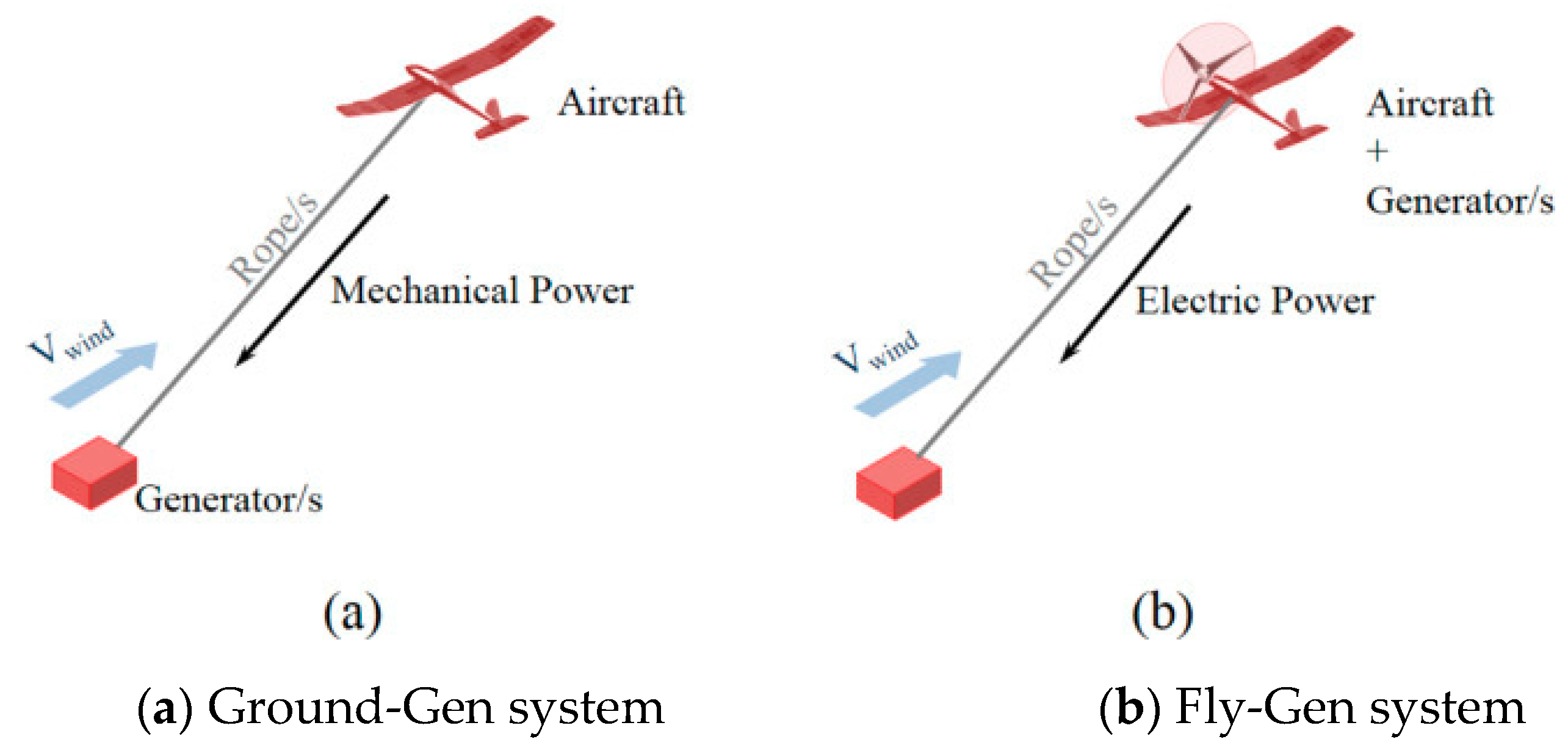
3. Application of a Tailored Tether to AWES

In this work, a tailored tether structure with characteristics of progressive failure (or yield-type failure response) was applied for the purpose of arresting an airborne wind energy system under snap loading; the analytical modeling of the failure response is described in this section.

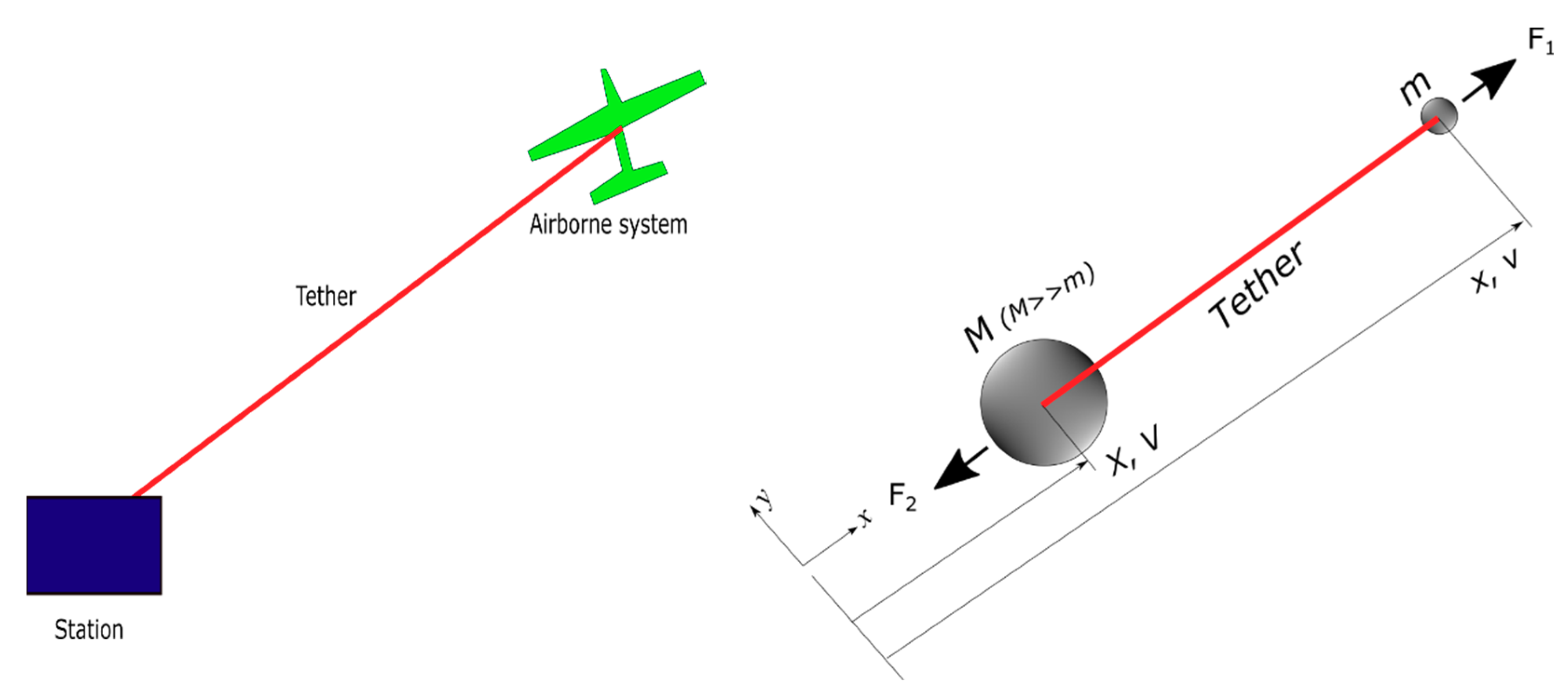
3.1. Simplification of an AWES with a Tailored Structure

The AWES model was simplified as a two-degree-of-freedom system with two longitudinally moving masses, M and m, and two masses connected by a tether, as shown in Figure 4.

The displacement and velocity components of an airborne system were represented as x (lower case) and v (lower case) and the station components as X (upper case) and V (upper case). In this study, only the longitudinal motion was considered. When the distance between the two masses is less than the total tether length, the effect of the external load on the structure is negligible. Otherwise—that is, when the distance between the two mass systems is greater than the tether length—the tether structure is subjected to impulsive (or snap) loading. The response of the tailored tether structure under impulsive loading was analytically modeled as described below.

3.2. Dynamic Response Model of Simplified AWES Model

Based on the simplified model shown in Figure 4, the motion of the airborne system (m) can be expressed by Equation (1) [23].

$$\begin{array}{ll}m\ddot{x}& =F_1-P\left(\delta \right)=F_1-K_i\left[\delta -\left(i-1\right)\left(l_s-l_p\right)\right]=F_1-K_i\left[u_1-u_2-\left(i-1\right)\left(l_s-l_p\right)\right]\\ & =F_1-K_i\left[x-X-L-\left(i-1\right)\left(l_s-l_p\right)\right]=F_1-K_i\left(x-X-L_i\right)\end{array}$$

(1)

where $P$ is the internal load, $\delta$ is the end displacement, p is the primary element, s is the secondary element, i is the failure stage, $L_i$ is the total tether length at the ith stage, $L_p$ is the tether length of the primary segment, $L_s$ is the tether length of the primary segment, $K_i$ is the equivalent tether stiffness at the ith stage, $u_1$ is the displacement of the mass m, and $u_2$ is the displacement of the mass M.

The equation of motion for the station system can also be similarly expressed as

$$M\ddot{X}=-F_2+P\left(\delta \right)=-F_2+K_i\left(x-X-L_i\right)$$

(2)

At the ith stage, the global motion of the two-degree-of-freedom system is given by following matrix form.

$$\begin{gathered} \left[\begin{array}{c}m0\\ 0M\end{array}\right]\left\{\begin{array}{c}\ddot{x}\\ \ddot{X}\end{array}\right\}+\left[\begin{array}{c}{K}_i-K_i\\ -K_i{K}_i\end{array}\right]\left\{\begin{array}{c}x\\ X\end{array}\right\}=\left\{\begin{array}{c}{F}_1+K_i{L}_i\\ -F_2-K_i{L}_i\end{array}\right\} \\ 1\le i\le \left(n+1\right),\left(x-X\right)\in \left(L+{\delta }_i^s,L+{\delta }_i^u\right] \end{gathered}$$

(3)

Therefore, the general solutions are

$$\begin{gathered} \begin{array}{ll}{x}_i\left(t\right)=q_{mi}\left(t\right)+& q_{Mi}\left(t\right)\\ & =\frac{1}{2}\frac{F_1-F_2}{m+M}{\left(t-{\tau }_i^0\right)}^2+A_i\left(t-{\tau }_i^0\right)+B_i+C_i\mathit{cos}{\omega }_i\left(t-{\tau }_i^0\right)+D_i\mathit{sin}{\omega }_i\left(t-{\tau }_i^0\right)\\ & +\frac{1}{m{\omega }_i{}^2}\left(K_i{L}_i+\frac{1}{1+\frac{m}{M}}\left(F_1+\frac{m}{M}{F}_2\right)\right)\end{array} \\ \begin{array}{ll}{X}_i\left(t\right)=& q_{mi}\left(t\right)-\frac{m}{M}{q}_{Mi}\left(t\right)=\frac{1}{2}\frac{F_1-F_2}{m+M}{(t-{\tau }_i^0)}^2+A_i\left(t-{\tau }_i^0\right)+B_i-\frac{m}{M}{C}_i\cos {\omega }_i\left(t-{\tau }_i^0\right)-\frac{m}{M}{D}_i\sin {\omega }_i\left(t-{\tau }_i^0\right)\\ & -\frac{1}{M{\omega }_i{}^2}\left(K_i{L}_i+\frac{1}{1+\frac{m}{M}}\left(F_1+\frac{m}{M}{F}_2\right)\right)\end{array} \end{gathered}$$

(4)

where, $q_{mi}\left(t\right)$ is the generalized coordinate of the mass m at the ith stage of the specific time t, $q_{Mi}\left(t\right)$ is the generalized coordinate of the mass M at the ith stage of the specific time t, and ${\omega }_i=\pm \sqrt{\frac{K_i\left(m+M\right)}{mM}}$.

At the ith stage, the initial conditions are

$$x_i\left({\tau }_i^0\right)=x_i{}^0,{\dot{x}}_i\left({\tau }_i^0\right)=v_i{}^0,X_i\left({\tau }_i^0\right)=X_i{}^0,{\dot{X}}_i\left({\tau }_i^0\right)=V_i{}^0$$

(5)

Given the initial conditions from Equation (5), the coefficients of Equation (4) are the following.

$$A_i=\frac{m{v}_i{}^0+M{V}_i^0}{m+M},B_i=\frac{m{x}_i^0+M{X}_i^0}{m+M},C_i=-\frac{K_i{L}_i\left(m+M\right)-mM{\omega }_i{}^2\left(x_i^0-X_i^0\right)+M{F}_1+m{F}_2}{m\left(m+M\right){\omega }_i^2},D_i=\frac{M\left(v_i^0-V_i^0\right)}{m\left(m+M\right){\omega }_i}$$

(6)

The maximum elongation at the ith stage is

$$\begin{array}{ll}{\delta }_i^{max}\left(t\right)& =x_i\left(t\right)-X_i\left(t\right)-L_i\\ & =\sqrt{{\left(C_i\left(1+\frac{m}{M}\right)\right)}^2+{\left(D_i\left(1+\frac{m}{M}\right)\right)}^2}\sin \left({\omega }_i\left(t-{\tau }_i^0\right)+{\alpha }_i\right)+\frac{F_1+\frac{m}{M}{F}_2}{K_i\left(1+\frac{m}{M}\right)}\end{array}$$

(7)

where, ${\alpha }_i=arctan\left(\frac{C_i}{D_i}\right)$ and $F_i^{max}=\{\begin{array}{c}{P}_p 1\le i\le n\\ P_s i=\left(n+1\right)\end{array}$.

The above equation is valid in the interval ${\tau }_i^0\le t\le {\tau }_i^f$, where the final time is given by

$${\tau }_i^f=\frac{1}{{\omega }_i}\{\begin{array}{c}\arcsin \frac{\frac{F_i^{max}}{K_i\frac{1}{K_i}\frac{F_1+\frac{m}{M}{F}_2}{1+\frac{m}{M}}}}{\sqrt{{\left(C_i\left(1+\frac{m}{M}\right)\right)}^2+{\left(D_i\left(1+\frac{m}{M}\right)\right)}^2}}\\ \end{array}-\arctan \left(\frac{C_i}{D_i}\right)\}$$

(8)

Subsequently, if ${\delta }_i^u>{\delta }_{i+1}^s$, the following equations of motion are obtained:

$$\begin{array}{c}m{\ddot{x}}_i=F_1\\ M{\ddot{X}}_i=-F_2\end{array}\}\Rightarrow \{\begin{array}{c}{\tilde{x}}_i=\frac{F_1}{2m}{\left(t-{\tau }_i{}^f\right)}^2+a_i\left(t-{\tau }_i{}^f\right)+b_i\\ {\tilde{X}}_i\left(t\right)=-\frac{F_2}{2M}{\left(t-{\tau }_i{}^f\right)}^2+c_i\left(t-{\tau }_i{}^f\right)+d_i\end{array},\left\{\begin{array}{c}\left(x-X\right)\in \left(L+{\delta }_i^u,L+{\delta }_{i+1}^s\right)\\ applicablefor{\tau }_i{}^f<t\le {\tilde{\tau }}_i^f\end{array}\right\}$$

(9)

with the initial conditions:

$$\begin{gathered} {\tilde{x}}_i\left({\tau }_i^f\right)=x_i\left({\tau }_i^f\right)=a_i{\tau }_i^f+b_i,{\dot{\tilde{x}}}_i\left({\tau }_i^f\right)={\dot{x}}_i\left({\tau }_i^f\right)=a_i \\ {\tilde{X}}_i\left({\tau }_i^f\right)=X_i\left({\tau }_i^f\right)=c_i{\tau }_i^f+d_i,{\dot{\tilde{X}}}_i\left({\tau }_i^f\right)={\dot{X}}_i\left({\tau }_i^f\right)=c_i \end{gathered}$$

(10)

Therefore, the solution to Equation (9) is given by

$$\begin{gathered} {\tilde{x}}_i\left(t\right)=\frac{F_1}{2m}{(t-{\tau }_i{}^f)}^2+{\dot{x}}_i\left({\tau }_i^f\right)\left(t-{\tau }_i^f\right)+x_i\left({\tau }_i^f\right) \\ {\tilde{X}}_i\left(t\right)=-\frac{F_1}{2M}{(t-{\tau }_i{}^f)}^2+{\dot{X}}_i\left({\tau }_i^f\right)\left(t-{\tau }_i^f\right)+X_i\left({\tau }_i^f\right) \end{gathered}$$

(11)

where ${\tilde{\tau }}_i^f$ is the solution to ${\tilde{x}}_i\left({\tilde{\tau }}_i^f\right)-{\tilde{X}}_i\left({\tilde{\tau }}_i^f\right)=L+{\delta }_{i+1}^s$

$${\tilde{\tau }}_i^f={\tau }_i^f+\frac{-\left({\dot{x}}_i\left({\tau }_i^f\right)-{\dot{X}}_i\left({\tau }_i^f\right)\right)+}{\frac{F_1}{m}+\frac{F_2}{M}}+\frac{\sqrt{{({\dot{x}}_i\left({\tau }_i^f\right)-{\dot{X}}_i\left({\tau }_i^f\right))}^2+2\left(\frac{F_1}{m}+\frac{F_2}{M}\right)\delta x_i}}{\frac{F_1}{m}+\frac{F_2}{M}}$$

(12)

where, $\delta x_i=L_{i+1}-(x_i({\tau }_i^f)-X_i({\tau }_i^f))$.

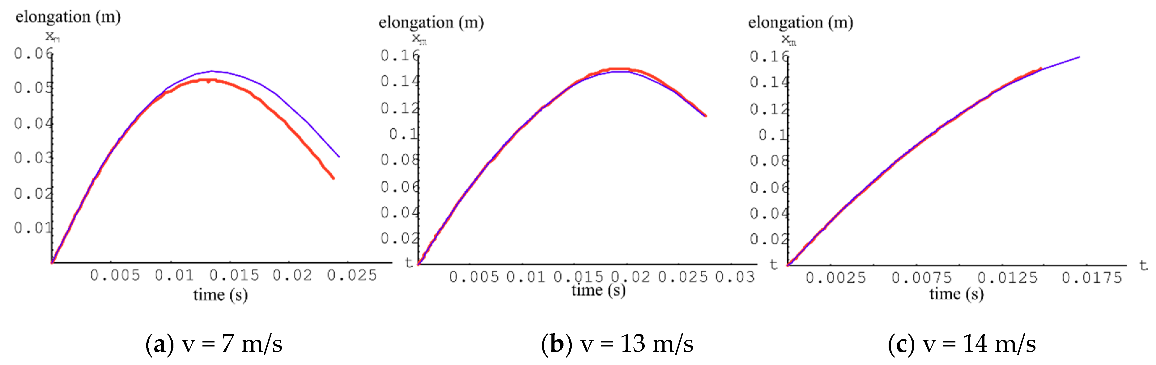
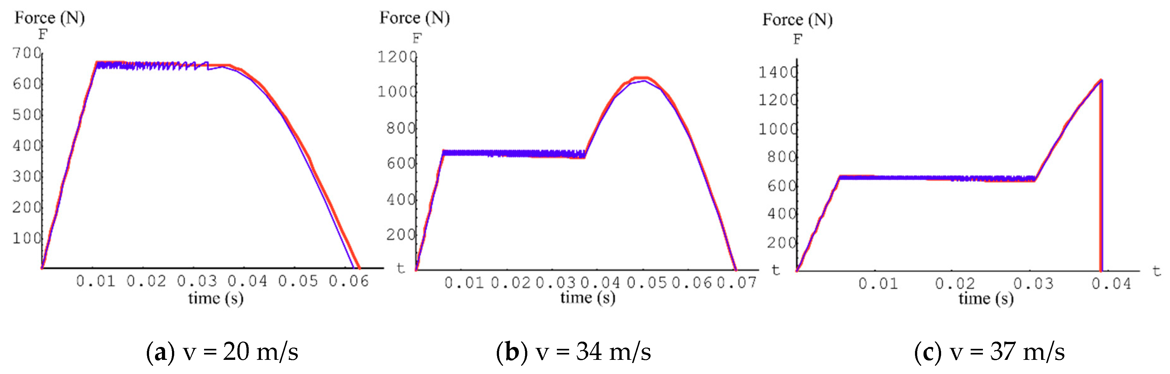
3.3. Approximate Response Modeling of Simplified AWES

In the previous section, the computation was executed whenever any elements failed, and the failure time and criteria were calculated at each step. For a very long tether, however, this requires expensive computational efforts. This section describes the approximate modeling of an AWES following the hypothesis that the mechanical work of an approximate response model should be close to one of the original models, as shown in Figure 5.

For an approximate response model, the parameters at each point, such as stiffness, force, and elongation, should be obtained. The stiffnesses of the tether at the first stage (I) and the last stage (III) are given by:

$$K_1=\frac{1}{\frac{1}{k_{cts}}+\frac{1}{k_s}+\frac{1}{k_{cps}}+\frac{n-1}{k_p}+\frac{n-2}{k_{cpp}}+\frac{1}{k_{ctp}}}, K_3=\frac{1}{\frac{2}{k_{cts}}+\frac{n}{k_s}+\frac{n-1}{k_{cps}}}$$

(13)

Fromthe approximate force-displacement relationship, the corresponding load values are expressed as:

$$F_1=K_1{\delta }_1,F_2=K_2\left({\delta }_2-\left(n+1-1\right)\left(l_s-l_p\right)\right), F_3=K_3\left({\delta }_3-\left(n+1-1\right)\left(l_s-l_p\right)\right)$$

(14)

Next, for the numerical computation, the responses are considered in detail for each stage.

Response at stage I

The equations of motion can be obtained according to the Euler–Lagrange equation $\frac{\partial }{\partial t}\left(\frac{\partial T}{\partial {\dot{q}}_i}\right)+\frac{\partial V}{\partial q_i}=Q_i$. Equation (15) expresses the kinetic and potential energy and the final equations are expressed in Equation (16) in matrix form.

$$\begin{gathered} T=\frac{1}{2}m{\dot{x}}_1^2+\frac{1}{2}M{\dot{X}}_1^2 \\ V=\frac{1}{2}{K}_1{\delta }^2=\frac{1}{2}{K}_1{(x_1-X_1-L)}^2 \end{gathered}$$

(15)

$$\left[\begin{array}{cc}m& 0\\ 0& M\end{array}\right]\left\{\begin{array}{c}{\ddot{x}}_1\\ {\ddot{X}}_1\end{array}\right\}+\left[\begin{array}{cc}{K}_1& -K_1\\ -K_1& K_1\end{array}\right]\left\{\begin{array}{c}{x}_1\\ X_1\end{array}\right\}=\left\{\begin{array}{c}{K}_{1}L\\ -K_{1}L\end{array}\right\}$$

(16)

Next, the forced vibration response of the tether at the first stage can be obtained as follows.

$$\begin{gathered} x_1\left(t\right)=q_m\left(t\right)+q_M\left(t\right)=A_1\left(t-{\tau }_0\right)+B_1+C_{1}cos{\omega }_1\left(t-{\tau }_0\right)+D_{1}sin{\omega }_1\left(t-{\tau }_0\right)+\frac{1}{m}\frac{K_{1}L}{{\omega }_1{}^2} \\ {X}_1\left(t\right)=q_m\left(t\right)-\frac{m}{M}{q}_M\left(t\right)=A_1\left(t-{\tau }_0\right)+B_1-\frac{m}{M}{C}_{1}cos{\omega }_1\left(t-{\tau }_0\right)-\frac{m}{M}{D}_{1}sin{\omega }_1\left(t-{\tau }_0\right)-\frac{1}{M}\frac{K_{1}L}{{\omega }_1{}^2} \end{gathered}$$

(17)

where ${\omega }_1{}^2=\frac{K_1}{m}\left(1+\frac{m}{M}\right)$.

By applying the initial conditions $x\left({\tau }_0\right)=x_0,\dot{x}\left({\tau }_0\right)=v_0,X\left({\tau }_0\right)=X_0,\dot{X}\left({\tau }_0\right)=V_0$ to Equation (17), we can obtain the coefficients.

$$A_1=\frac{m{v}_0+M{V}_0}{m+M}, B_1=\frac{m{x}_0+M{X}_0}{m+M}, C_1=-\frac{K_{1}L\left(m+M\right)-mM{\omega }^2\left(x_0-X_0\right)}{m\left(m+M\right){\omega }_1^2}, D_1=\frac{M\left(v_0-V_0\right)}{\left(m+M\right){\omega }_1}$$

(18)

Response at stage II

The tether response at stage II is shown in Figure 6.

In Figure 6,

$$K_2=\frac{1}{\frac{2}{K_{cts}}+\frac{N}{K_s}+\frac{N-1}{K_{css}}}, K_d=-\frac{F_2-F_1}{{\delta }_2-{\delta }_1}, F_2=K_2\left({\delta }_2-N\right)\left(l_s-l_p\right)$$

(19)

Since the response of the second stage (II) is inelastic, the virtual work resulting from nonconservative force needs to be plugged into the Lagrange equation.

$$\begin{array}{ll}\delta W& =F_{ext}\overrightarrow{i}\times \delta \left(\Delta \right)=-\left[F_1-K_d\left(\Delta -{\delta }_1\right)\right]\overrightarrow{i}\times \delta \left(\Delta \right)=-\left[F_1-K_d\left(x-X-L-{\delta }_1\right)\right]\overrightarrow{i}\times \left(\delta x_2-\delta X_2\right)\overrightarrow{i}\\ & =-\left[F_1-K_d\left(x_2-X_2-L-{\delta }_1\right)\right]\delta x_2+\left[F_1-K_d\left(x_2-X_2-L-{\delta }_1\right)\right]\delta X_2=Q_1\delta x_2+Q_2\delta X_2\end{array}$$

(20)

Based on the rule of Euler–Lagrange’s equation, $\frac{\partial }{\partial t}\left(\frac{\partial T}{\partial {\dot{q}}_i}\right)+\frac{\partial V}{\partial q_i}=Q_i$, the equations of motion are given by:

$$\left[\begin{array}{cc}m& 0\\ 0& M\end{array}\right]\left\{\begin{array}{c}{\ddot{x}}_2\\ {\ddot{X}}_2\end{array}\right\}-\left[\begin{array}{cc}{K}_d& -K_d\\ -K_d& K_d\end{array}\right]\left\{\begin{array}{c}{x}_2\\ X_2\end{array}\right\}=\left\{\begin{array}{c}-F_1-K_d\left(L+{\delta }_1\right)\\ F_1+K_d\left(L+{\delta }_1\right)\end{array}\right\}$$

(21)

Next, the forced vibration response can be obtained as follows:

$$\begin{gathered} x_2\left(t\right)=q_m\left(t\right)+q_M\left(t\right)=A_2\left(t-{\tau }_{f1}\right)+B_2+C_{2}Exp\left({\omega }_2\left(t-{\tau }_{f1}\right)\right)+D_{2}Exp\left(-{\omega }_2\left(t-{\tau }_{f1}\right)\right)\frac{1}{m}\frac{1}{{\omega }_2{}^2}\left[F_1+K_d\left({\delta }_1+L\right)\right] \\ {X}_2\left(t\right)=q_m\left(t\right)-\frac{m}{M}{q}_M\left(t\right)=A_2\left(t-{\tau }_{f1}\right)+B_2-\frac{m}{M}{C}_{2}Exp\left({\omega }_2\left(t-{\tau }_{f1}\right)\right)-\frac{m}{M}{D}_{2}Exp\left(-{\omega }_2\left(t-{\tau }_{f1}\right)\right)-\frac{m}{M}\frac{1}{m}\frac{1}{{\omega }_2{}^2}\left[F_1+K_d\left({\delta }_1+L\right)\right] \end{gathered}$$

(22)

where ${\omega }_2{}^2=\frac{K_d}{m}\left(1+\frac{m}{M}\right)$ (14).

By applying the initial conditions $x_2\left({\tau }_{f1}\right)=x_{f1},$ ${\dot{x}}_2\left({\tau }_{f1}\right)=v_{f1}, X_2\left({\tau }_{f1}\right)=X_{f1},{\dot{X}}_2\left({\tau }_{f1}\right)=V_{f1}$ to Equation (22), we can obtain the coefficients:

$$\begin{gathered} A_2=\frac{m{v}_{f1}+M{V}_{f1}}{m+M}, B_2=\frac{m{x}_{f1}+M{X}_{f1}}{m+M}, \\ {C}_2=-\left[\begin{array}{l}\left(m+M\right)F_1+mM{\omega }_2\left[-{\omega }_2\left(x_{f1}-X_{f1}\right)-\left(v_{f1}-V_{f1}\right)\right]\\ +\left(m+M\right)K_d\left(L+{\delta }_1\right)\end{array}\right]/\left[m\left(m+M\right){\omega }_1^2\right] \\ {D}_2=-\left[\begin{array}{l}\left(m+M\right)F_1+mM{\omega }_2\left[-{\omega }_2\left(x_{f1}-X_{f1}\right)+\left(v_{f1}-V_{f1}\right)\right]\\ +\left(m+M\right)K_d\left(L+{\delta }_1\right)\end{array}\right]/\left[m\left(m+M\right){\omega }_1^2\right] \end{gathered}$$

(23)

Tether status check at stage II

The tether failure can be checked according to the work–energy theorem.

$$\begin{array}{ll}-W& =\left(Total Area\right)=A_{126}+A_{2346}-A_{345}\\ & =\frac{1}{2}{F}_1{\delta }_1+{{\displaystyle \int }}_{{\delta }_1}^{{\delta }^{*}}\left[F_1-K_d\left(\delta -{\delta }_1\right)\right]d\delta -{{\displaystyle \int }}_d^{{\delta }^{*}}\left[F^{*}+K_1\left(\delta -{\delta }^{*}\right)\right]d\delta \end{array}$$

(24)

where ${\delta }^{*}=x_2\left(t^{*}\right)-X_2\left(t^{*}\right)-L,F^{*}=F_1-K_d\left({\delta }^{*}-{\delta }_1\right),andd=\frac{F^{*}}{K_1}+{\delta }^{*}$

The kinetic energy variation can be expressed as:

$$\Delta T=T^{*}-T_0=\frac{1}{2}m\left(v_{*}{}^2+V_{*}{}^2\right)-\frac{1}{2}m\left(v_0{}^2+V_0{}^2\right)$$

(25)

In cases in which the kinetic energy variation of the moving flying object (m) is higher than the amount of work produced by the external force and elongation (${\delta }_2$), all the main elements will fail.

Response at the second stage (II) when the failure of primary elements occurs

The corresponding response at the second stage when some of the primary elements fail is as follows:

$$\begin{array}{ll}{x}_3\left(t\right)=q_m\left(t\right)+& q_M\left(t\right)\\ & =A_3\left(t-{\tau }_{f2}\right)+B_3+C_{3}cos{\omega }_3\left(t-{\tau }_{f2}\right)+D_{3}sin{\omega }_3\left(t-{\tau }_{f2}\right)\\ & +\frac{1}{m{\omega }_3{}^2}\left[-F^{*}+K_1\left({\delta }^{*}+L\right)\right]\\ X_3\left(t\right)=q_m\left(t\right)-& \frac{m}{M}{q}_M\left(t\right)\\ & =A_3\left(t-{\tau }_{f2}\right)+B_3-\frac{m}{M}{C}_{3}cos{\omega }_3\left(t-{\tau }_{f2}\right)-\frac{m}{M}{D}_{3}sin{\omega }_3(t\\ & -{\tau }_{f2})-\frac{m}{M}\frac{1}{m{\omega }_3{}^2}\left[-F^{*}+K_1\left({\delta }^{*}+L\right)\right]\end{array}$$

(26)

where ${\omega }_3{}^2=\frac{\left(m+M\right)K_1}{mM}$.

By applying the initial conditions $x_3\left({\tau }_{f2}\right)=x_{f2},$ ${\dot{x}}_3\left({\tau }_{f2}\right)=v_{f2},X_3\left({\tau }_{f2}\right)=X_{f2},{\dot{X}}_3\left({\tau }_{f2}\right)=V_{f2}$ to Equation (26), we can obtain the coefficients:

$$\begin{gathered} A_3=\frac{m{v}_2^{*}+M{V}_2^{*}}{m+M}, B_3=\frac{m{x}_2^{*}+M{X}_2^{*}}{m+M} \\ {C}_3=\frac{\left(m+M\right)F^{*}+mM{\omega }_3{}^2\left(x_2^{*}-X_2^{*}\right)-K_1\left({\delta }^{*}+L\right)\left(m+M\right)}{m\left(m+M\right){\omega }_3^2},D_3=\frac{M(v_2^{*}-V_2^{*}}{\left(m+M\right){\omega }_3^{}} \end{gathered}$$

(27)

The final time is given by:

$${\tau }_{f3}={\tau }_{f2}+\frac{1}{{\omega }_3}\left[\pi -ArcSin\left(0\right)-ArcTan\left(\frac{C_3}{D_3}\right)\right]$$

(28)

Response at the last stage (III)

The corresponding response at the last stage when some of primary elements fail is as follows:

$$\begin{array}{ll}{x}_3\left(t\right)=q_m\left(t\right)+& q_M\left(t\right)\\ & =A_3\left(t-{\tau }_{f2}\right)+B_3+C_{3}cos{\omega }_3\left(t-{\tau }_{f2}\right)+D_{3}sin{\omega }_3\left(t-{\tau }_{f2}\right)\\ & +\frac{1}{m{\omega }_3{}^2}\left[-F_2+K_3\left({\delta }_2+L\right)\right]\\ X_3\left(t\right)=q_m\left(t\right)-& \frac{m}{M}{q}_M\left(t\right)\\ & =A_3\left(t-{\tau }_{f2}\right)+B_3-\frac{m}{M}{C}_{3}cos{\omega }_3\left(t-{\tau }_{f2}\right)-\frac{m}{M}{D}_{3}sin{\omega }_3(t\\ & -{\tau }_{f2})-\frac{m}{M}\frac{1}{m{\omega }_3{}^2}\left[-F_2+K_3\left({\delta }_2+L\right)\right]\end{array}$$

(29)

where ${\omega }_3{}^2=\frac{\left(m+M\right)K_3}{mM}$.

By applying the initial conditions $x_3\left({\tau }_{f2}\right)=x_{f2},{\dot{x}}_3\left({\tau }_{f2}\right)=v_{f2},X_3\left({\tau }_{f2}\right)=X_{f2}, {\dot{X}}_3\left({\tau }_{f2}\right)=V_{f2}$ to Equation (29), we can obtain the coefficients:

$$\begin{gathered} A_3=\frac{m{v}_{f2}+M{V}_{f2}}{m+M},B_3=\frac{m{x}_{f2}+M{X}_{f2}}{m+M}, \\ {C}_3=\frac{\left[\left(m+M\right)F_2+mM{\omega }_3{}^2\left(x_{f2}-X_{f2}\right)-K_5\left({\delta }_2+L\right)\left(m+M\right)\right]}{m\left(m+M\right){\omega }_3^2},D_3=\frac{m(v_2^{}-V_2^{})}{\left(m+M\right){\omega }_3^{}} \end{gathered}$$

(30)

4. Numerical Results

Figure 7 and Figure 8 show the comparison plots of the approximate and the full response of the tether structure. The higher the initial velocities were, the closer the approximate response was to the full response result. Also, as shown in Figure 9, Figure 10, Figure 11 and Figure 12, the approximate solutions demonstrated very good correlation to the full response results as the number of elements, that is, the length of tether, increased from N = 15 to N = 1000. The benefit of the approximate solution concerns the computational cost. For N = 1000, the computation time was just 5 s while the full analytical results took about 10 min. Even for N = 10,000 elements, the approximate model took 10 s while the fully analytical model took more than an hour.

5. Conclusions

The applicability and benefits of a tailored tether for an airborne wind energy system (AWES) were investigated. The AWES system with a tether structure was simplified as a two-degree-of-freedom system and an exact response was mathematicallyobtained. The composite tether was proven to show better endurance under impulsive loading compared to the conventional structure since more mechanical work was required to reach complete structure failure, thanks to the multiple load paths (primary and secondary elements). Furthermore, an approximate response model was developed, which resulted in a dramatic reduction of computational cost as well as showing good correlation with the original results.

References

1. Handayani, K.; Krozer, Y.; Filatova, T. From fossil fuels to renewables: An analysis of long-term scenarios considering technological learning. Energy Policy 2019, 127, 134–146. [Google Scholar] [CrossRef]
2. Herbert, G.M.J.; Iniyan, S.; Sreevalsan, E.; Rajapandian, S. A review of wind energy technologies. Renew. Sustain. Energy Rev. 2007, 11, 1117–1145. [Google Scholar] [CrossRef]
3. de Lellis, M.; Reginatto, R.; Saraiva, R.; Trofino, A. The Betz limit applied to airborne wind energy. Renew. Energy 2018, 127, 32–40. [Google Scholar] [CrossRef]
4. Konstantinidis, E.I.; Botsaris, P.N. Wind Turbines: Status, obstacles, trends, and technologies. IOP Conf. Ser. Mater. Sci. Eng. 2016, 161, 012079. [Google Scholar] [CrossRef]
5. Sirnivas, S.; Musial, W.; Bailey, B.; Filippelli, M. Assessment of Offshore Wind System Design, Safety, and Operation Standards; NREL/TP-5000-60573; National Renewable Energy Laboratory: Golden, CO, USA, 2014. [Google Scholar]
6. Korchinski, W. The Limits of Wind Power; Reason Foundation and Cascade Policy Institute: Portland, OR, USA, 2012; Available online: http://cascadepolicy.org/pdf/pub/Oregon_Limits_of_Wind_Power.pdf (accessed on 26 April 2013).
7. Diehl, M. Airborne wind energy: Basic concepts and physical foundations. In Airborne Wind Energy. Green Energy and Technology; Ahrens, U., Diehl, M., Schmehl, R., Eds.; Springer: Berlin/Heidelberg, Germany, 2013. [Google Scholar] [CrossRef]
8. Vermillion, C.; Glass, B.; Rein, A. Lighter-than-air wind energy systems. In Airborne Wind Energy. Green Energy and Technology; Ahrens, U., Diehl, M., Schmehl, R., Eds.; Springer: Berlin/Heidelberg, Germany, 2013. [Google Scholar] [CrossRef]
9. Roberts, B.W.; Shepard, D.H.; Caldeira, K.; Cannon, M.E.; Eccles, D.G.; Grenier, A.J.; Freidin, J.F. Harnessing high-altitude wind power. IEEE Trans. Energy Convers. 2007, 22, 136–144. [Google Scholar] [CrossRef] [Green Version]
10. Lunney, E.; Ban, M.; Duic, N.; Foley, A. A state-of-the-art review and feasibility analysis of high altitude wind power in Northern Ireland. Renew. Sustain. Energy Rev. 2017, 68, 899–911. [Google Scholar] [CrossRef] [Green Version]
11. Ahrens, U.; Diehl, M.; Schmehl, R. Airborne Wind Energy; Springer: Berlin/Heidelberg, Germany, 2013. [Google Scholar] [CrossRef]
12. Cherubini, A.; Papini, A.; Vertechy, R.; Fontana, M. Airborne wind energy systems: A review of the technologies. Renew. Sustain. Energy Rev. 2015, 51, 1461–1476. [Google Scholar] [CrossRef] [Green Version]
13. Argatov, I.; Rautakorpi, P.; Silvennoinen, R. Apparent wind load effects on the tether of a kite power generator. J. Wind Eng. Ind. Aerodyn. 2011, 99, 1079–1088. [Google Scholar] [CrossRef]
14. Dunker, S. Tether and Bridle Line Drag in Airborne Wind Energy Applications; Springer: Berlin/Heidelberg, Germany, 2018. [Google Scholar] [CrossRef]
15. Salma, V.; Friedl, F.; Schmehl, R. Improving reliability and safety of airborne wind energy systems. Wind Energy 2020, 23, 340–356. [Google Scholar] [CrossRef] [Green Version]
16. Dancila, D.S.; Armanios, E.A. Energy-dissipating composite members with progressive failure: Concept development and analytical modeling. AIAA J. 2002, 40, 2096–2104. [Google Scholar] [CrossRef]
17. Majak, J.; Hannus, S. Orientational design of anisotropic materials using the hill and tsai–wu strength criteria. Mech. Compos. Mater. 2003, 39, 509–520. [Google Scholar] [CrossRef]
18. Lellep, J.; Majak, J. On optimal orientation of nonlinear elastic orthotropic materials. Struct. Optim. 1997, 14, 116–120. [Google Scholar] [CrossRef]
19. Dababneh, O.; Kipouros, T.; Whidborne, J.F. Application of an efficient gradient-based optimization strategy for aircraft wing structures. Aerospace 2018, 5, 3. [Google Scholar] [CrossRef] [Green Version]
20. Majak, J.; Pohlak, M.; Eerme, M. Design of car frontal protection system using neural networks and genetic algorithm. Mechanika 2012, 18, 453–460. [Google Scholar] [CrossRef] [Green Version]
21. Kers, J.; Majak, J.; Goljandin, D.; Gregor, A.; Malmstein, M.; Vilsaar, K. Extremes of apparent and tap densities of recovered GFRP filler materials. Compos. Struct. 2010, 92, 2097–2101. [Google Scholar] [CrossRef]
22. Dancila, D.S.; Armanios, E.A. Energy Dissipating Composite Members with Progressive Failure. U.S. Patent No. 6,136,406, 24 October 2000. [Google Scholar]
23. Bauchau, O.A. Flexible Multibody Dynamics; Springer: Dordrecht, The Netherlands; Heidelberg, Germany; London, UK; New-York, NY, USA, 2010; ISBN 978-94-007-0334-6. [Google Scholar]
Figure 1. Examples of airborne wind energy systems (AWES) [12].
Applsci 11 00166 g001
Figure 2. A schematic concept of a tether structure (a) and its physically manufactured example (b).
Applsci 11 00166 g002
Figure 3. Comparison of response prediction.
Applsci 11 00166 g003
Figure 4. Simplified AWES model connected with a composite tether.
Applsci 11 00166 g004
Figure 5. Approximation technique for tether response of an AWES.
Applsci 11 00166 g005
Figure 6. Force and displacement plot for the first and second stages.
Applsci 11 00166 g006
Figure 7. Forced responses at various initial velocities (v = 7 m/s, 13 m/s, 14 m/s). Number of segments = 15, red line: approximate solution, blue line: exact solution.
Applsci 11 00166 g007
Figure 8. Elongations at various initial velocities (v = 7 m/s, 13 m/s, 14 m/s). Number of segments = 15, red line: approximate solution, blue line: exact solution.
Applsci 11 00166 g008
Figure 9. Forced responses at various initial velocities (v = 20 m/s, 34 m/s, 37 m/s). Number of segments = 100, red line: approximate solution, blue line: exact solution.
Applsci 11 00166 g009
Figure 10. Elongations at various initial velocities (v = 20 m/s, 34 m/s, 37 m/s). Number of segments = 100, red line: approximate solution, blue line: exact solution.
Applsci 11 00166 g010
Figure 11. Forced responses at various initial velocities (v = 70 m/s, 113 m/s, 114 m/s). Number of segments = 1000, red line: approximate solution, blue line: exact solution.
Applsci 11 00166 g011
Figure 12. Elongations at various initial velocities (v = 70 m/s, 113 m/s, 114 m/s). Number of segments = 1000, red line: approximate solution, blue line: exact solution.
Applsci 11 00166 g012
Publisher’s Note: MDPI stays neutral with regard to jurisdictional claims in published maps and institutional affiliations.