Abstract
Due to the rapid progress in the development of automated vehicles over the last decade, their market entry is getting closer. One of the remaining challenges is the safety assessment and type approval of automated vehicles, as conventional testing in the real world would involve an unmanageable mileage. Scenario-based testing using simulation is a promising candidate for overcoming this approval trap. Although the research community has recognized the importance of safeguarding in recent years, the quality of simulation models is rarely taken into account. Without investigating the errors and uncertainties of models, virtual statements about vehicle safety are meaningless. This paper describes a whole process combining model validation and safety assessment. It is demonstrated by means of an actual type-approval regulation that deals with the safety assessment of lane-keeping systems. Based on a thorough analysis of the current state-of-the-art, this paper introduces two approaches for selecting test scenarios. While the model validation scenarios are planned from scratch and focus on scenario coverage, the type-approval scenarios are extracted from measurement data based on a data-driven pipeline. The deviations between lane-keeping behavior in the real and virtual world are quantified using a statistical validation metric. They are then modeled using a regression technique and inferred from the validation experiments to the unseen virtual type-approval scenarios. Finally, this paper examines safety-critical lane crossings, taking into account the modeling errors. It demonstrates the potential of the virtual-based safeguarding process using exemplary simulations and real driving tests.
1. Introduction
Automated driving is a major trend in the automotive industry as it promises to increase road safety and driver comfort. In 2018, more than one million people died in road accidents [1]. National governments are striving to increase the level of vehicle automation to reduce these figures. Advanced Driver Assistance Systems (ADAS) (Level 1 according to SAE [2]) such as emergency braking or lane-keeping assists are common in modern vehicles and will be mandatory in Europe beginning in 2022 [3]. On the one hand, car manufacturers have a high responsibility to dedicate a significant part of the development process to the safety assessment of those systems. On the other hand, the United Nations Economic Commission for Europe (UNECE) is developing type-approval regulations to ensure that these systems meet important safety requirements before they are finally released to the market [4,5].
In recent years, the safety assessment of automated vehicles (AVs) has been very much addressed in the literature and large research projects [6,7], as it is a huge challenge due to the complexity of the traffic environment. Conventional testing in the physical world struggles with higher automation levels, since it requires an enormous amount of mileage to prove that an AV is at least as safe as a human driver [8]. A promising solution is the scenario-based approach. It discards the major part of the mileage that lacks interesting actions and events and focuses instead on a selection of individual traffic situations [9]. There is a large number of publications that propose scenario generation approaches for safety assessment of AVs. Some extract the scenarios from driving data [10,11], others generate the scenarios from scratch [12], for example using Design of Experiments (DoE) techniques [13].
While conventional tests are physically performed on the road, more recent publications use pure simulations for their proof of concept. They convince by cost and effort reduction, increased safety and possible parallelization through computing clusters. Nevertheless, the simulations have to be accompanied by model validation activities in order to achieve trustworthiness. The combination of model validation and virtual safeguarding leads to an overall virtual-based process. This process uses physical tests to assess the quality of the simulation during model validation in order to finally exploit the strength of the simulation in virtual safeguarding [14]. The current literature focuses on safeguarding and, within safeguarding, on the selection of scenarios. However, an overall virtual-based process including model validation and including the selection of additional validation scenarios is missing. We address these research gaps in this paper.
Our main contributions are as follows:
- an overview about methods to select test scenarios for AVs and methods to assign them to testing environments,
- a novel approach to select both scenarios for model validation and for safeguarding,
- a methodology for virtual-based safeguarding of AVs based on real and virtual tests,
- first implementation with a real and virtual prototype vehicle using the type approval of lane keeping systems as a representative safety assessment example.
Section 2 summarizes the state-of-the-art in type approval and model validation, as well as scenario selection and assignment. It concludes with an analysis of the strengths and weaknesses of the scenario generation methods and makes a reasoned selection. Section 3 embeds the scenario approaches in an overall, virtual-based safety assessment process. It presents a coverage-based approach to generate validation scenarios and a data-driven approach to extract safeguarding scenarios. It processes the validation results using a probabilistic validation metric, learns an error model and takes the modeling errors into account during the final decision making. Section 4 illustrates the methodology by an exemplary type-approval regulation of a lane-keeping system across a real and virtual test environment. Lastly, the conclusion in Section 5 summarizes the main research findings and gives recommendations for virtual-based safety assessment.
2. Literature Overview
This section presents a literature overview in a top-down manner. It starts with the type approval of lane-keeping systems as a representative example for safety assessment. It continues with model validation references as they are crucial for virtual-based type approval and safety assessment in general. The third subsection zooms into the model validation methodology to introduce papers that select validation scenarios. Since these papers are rare, we additionally present scenario selection approaches from virtual safeguarding. Finally, we analyze the scenario approaches to derive a systematic selection for our subsequent methodology. Thus, this section gives the reader a compact overview of scenario-based safety assessment and model validation. Complementary safety approaches such as formal verification methods or macroscopic traffic simulations do not fall within the scope of this paper. The interested reader is referred to [14] for a comprehensive overview.
2.1. Type Approval of Lane-Keeping Systems
The UNECE specifies several mandatory type-approval regulations. Some of them allow computer simulation if accompanied by model validation [15,16]. The future regulation for Automated Lane-Keeping Systems (ALKS) of SAE Level 3 falls into this category by stating:
Simulation tool and mathematical models for verification of the safety concept may be used [...]. Manufacturers shall demonstrate [...] the validation performed for the simulation tool chain (correlation of the outcome with physical tests).[5] Section 4.2
The predecessor regulation R-79 [4], which deals with continuously intervening lane-keeping systems as installed in many production vehicles of SAE Levels 1 and 2, is currently carried out by physical tests. Nevertheless, we select R-79 as the most suitable use case for a virtual-based type approval in this paper. We do not actually intend to release a vehicle to the market by precisely implementing the regulation. We have a Level 2 vehicle available and use the corresponding R-79 as a blueprint to develop a methodology for future virtual-based type approval [5].
The regulation describes several tests for the lane-keeping assessment of several vehicle classes and system states. The current Revision 4 of R-79 is supplemented by further amendments that provide remarks on specific aspects such as signal filtering [17]. To illustrate our methodology on a specific example that focuses on the intended functionality of the lane-keeping assist, we choose the Lane-Keeping Functional Test (LKFT) shown in Figure 1. One goal of this test is to guide the vehicle into a quasi-stationary condition of the lateral acceleration within the range from 80% to 90% of the maximum lateral acceleration specified by the vehicle manufacturer. Nevertheless, the regulation requires proof “for the whole lateral acceleration and speed range”([4], Section 3.2.1.3). Therefore, we will directly focus on a good coverage of the entire scenario space across both dimensions.

Figure 1.
Schematic overview of the Lane-Keeping Functional Test.
Within these quasi-stationary ranges, it has to be checked whether the vehicle crosses or even touches the lane boundary and whether the change in movement is within defined limits. In a previous publication [18], we presented an approach to determine the distance to line y of the vehicle edges with high precision in post-processing. This makes it possible to determine the position of the vehicle on public roads with an accuracy of a few centimeters [19]. According to the test specifications, the driver is taken out of the loop by briefly removing his hands from the steering wheel. The criterion of crossing the lane boundary represents an important safety aspect, since serious consequences can occur if the vehicle leaves the lane.
2.2. Model Validation
Since models have a long history and are used in numerous application areas, there is a myriad of literature on model validation. We gave a comprehensive survey about model Verification, Validation and Uncertainty Quantification (VV&UQ) approaches in [20]. We developed a generic modular framework and embedded most of the literature approaches and application areas within it. At this point, we highlight individual aspects that are integral to this paper’s central theme and understanding. The interested reader is referred to [20] regarding a more detailed introduction and theory. In the later sections, we will present this framework in a specific manifestation for the virtual-based safeguarding of AVs. In this section, we present approaches that can be used as a basis to configure the framework.
The state-of-the-art in automotive model validation tends to focus on single components such as environmental sensor models [21,22,23] or vehicle dynamics models [24,25], but rarely on the overall closed-loop behavior [26,27]. Since these exemplary references all focus on specific effects such as the influence of sensor artifacts, they are important for increasing the credibility of the models, but are not sufficient for the virtual safety assessment of the entire vehicle. Therefore, with respect to scenario selection, we build on the automotive literature of the previous subsections. However, we consider advanced methods from other application fields as a basis for our validation methodology. In general, one promising example is the work of Oberkampf and Roy [28] on Probability Bound Analysis (PBA) in the field of Computational Fluid Dynamics (CFD).
Several validation metrics are available to quantify the difference between simulation and reality in the form of scalar values [25], time series [29] or probability distributions [30]. In addition, there are various metamodeling techniques such as polynomial regression [28] or Gaussian processes [31] to represent the validation errors. Finally, recent references [28,32,33] focus on the aggregation of modeling errors and uncertainties from validation experiments to the intended use of the model. This is quite a challenge [34], but especially important since the application-specific decisions are made based on the erroneous simulation models. We will consider these central aspects in the further course of this paper.
2.3. Scenario Assignment Methods
There are a few references that assign scenarios to real and virtual test environments. Since they are relevant for the selection of validation scenarios, we present them in more detail. The paper by Schuldt et al. [35] presents a first idea of how a use case can be assigned to different X-in-the-Loop (XiL) approaches. The authors use components of the AV as dimensions in a Kiviat diagram and distinguish three steps for each component: simulated, emulated and physically present. In addition, they propose quality functionals to consider and weight certain influencing factors such as the quality of results or costs. They describe both the XiL approaches and the use case of a construction site assistant using the Kiviat diagrams. Since only the Vehicle-in-the-Loop approach meets the requirements of their use case, they choose this approach as their test environment.
Böde et al. [36] aim to find an optimal split between the number of scenarios in simulation and the real world. They decompose the probability that the system satisfies its requirements into two terms based on the law of total probability. The first term describes the probability that the model satisfies the system requirements. It is conditioned on the second term with the probability that the model is a valid representation. They consider also a statistical uncertainty due to sampling of test scenarios. They propose three notions of model validity: all observed trajectories are possible in simulation and lead to the same decisions, each virtual trajectory has at least one physical counterpart, or the likelihood of the virtual and physical trajectories is identical. They select the first and weakest notion and assume that both probabilities are one, which means that all tests are passed and the model is valid, so that only the statistical uncertainty remains. Then they calculate the optimal number of scenarios in simulation and the real world for different costs of both environments.
Beyond automated driving, there is generally little literature available regarding the split between test environments. Morrison et al. [37], Terejanu [38] find an optimal split between physical data to be used for model calibration and validation. Mullins et al. [39] similarly find the optimal number of calibration and validation tests considering both the costs at each test condition and the prediction uncertainty of the simulation model. They use a probabilistic simulation in a Bayesian framework. Model calibration reduces the uncertainty in the posterior distribution of the model parameters. In contrast, model validation again adds uncertainty to the parameters using an overall reliability metric to account for model inadequacy and sparse data, but it reduces the uncertainty about the model prediction itself. They formulate a joint optimization that selects the number of tests so that the costs and the future prediction uncertainty of the model are minimized.
2.4. Scenario Selection Methods
Since there are only a few references addressing the assignment of scenarios to test environments, but quite a variety of methods for generating scenarios for safeguarding, we extend the literature review to the latter area of research. This subsection provides an overview about four types of scenario selection approaches. Each of these approaches has already been implemented in different variants in several references. We select representative references from these to provide a common basis for this paper. Detailed information can be found in [14] and in the respective papers.
2.4.1. Knowledge-Based Methods
Knowledge-based approaches use abstract information in the form of standards, guidelines or expert knowledge as a source for the generation of scenarios. An exemplary source is the German guideline for the construction of motorways [40]. Most knowledge-based approaches are based on ontologies. They can represent knowledge, model properties and relationships and automatically generate test scenarios that constitute valid combinations. This is a crucial advantage compared to simpler approaches like pure combinatorial testing. Chen and Kloul [41] combine a motorway, a weather and a vehicle ontology and also model the relationships between the three ontologies. Bagschik et al. [9] concentrate on German highways and represent all five layers of their environmental model. Li et al. [42] use an ontology as input for combinatorial testing in a multi-step process.
2.4.2. Data-Driven Methods
Data-driven methods extract scenarios from data that are normally recorded during test drives with a fleet of vehicles equipped with special measurement technology. In the post-processing step, machine learning and pattern recognition techniques are applied to the recorded data. Some papers extract concrete scenarios from the data that have a high novelty value. For example, Langner et al. [10] use an autoencoder, as its reproduction error can be interpreted as a novelty indicator. Krajewski et al. [11] extend the idea and use generative neural networks such as a Generative Adversarial Network (GAN) and a Variational Autoencoder (VAE) to not only extract existing scenarios, but also to generate new ones from them.
Further papers aimed to parameterize scenarios with parameter ranges and distributions. Therefore, similar scenarios are grouped together in a first processing step. Either specific scenario classes such as following, lane change or cutting-in are defined to use supervised learning techniques to assign the data to the classes [43,44], or the data are clustered based on similarity using unsupervised learning techniques [45,46]. Afterwards, the grouped data can be used to parameterize the scenarios. Zhou and del Re [47] parameterize a lane-change maneuver with a hyperbolic tangent function. Similar work fitting a distribution to a car-following scenario using Kernel Density Estimation (KDE) can be found in [48].
2.4.3. Coverage-Based Methods
Coverage-based methods generate a set of test scenarios that cover the scenario space well. They sample concrete scenarios [49] either from parameter ranges or parameter distributions. The latter has the advantage that the distributions provide the occurrence probability of a scenario and thus its relevance in the real world. A wide variety of sampling techniques was already applied to generate scenarios from parameter ranges, for example, Design of Experiments (DoE) [13], Satisfiability Modulo Theory (SMT) solvers [50], Rapidly Exploring Random Trees (RRTs) [12] or the In-Parameter-Order-Generalized (IPOG) algorithm [51]. Distributional sampling techniques are based on Monte Carlo methods. Most papers use accelerated techniques to cope with the fact that critical traffic scenarios are rare events. For instance, Zhao [52] uses Importance Sampling (IS) to speed-up the computation, and Åsljung et al. [53] use Extreme Value Theory (EVT).
2.4.4. Falsification-Based Methods
Falsification-based methods focus on optimization techniques in order to obtain more challenging scenarios. Some papers use accident databases as a starting point [54]. Other papers define criticality metrics or complexity metrics to quantify scenario properties. For example, Klischat and Althoff [55] calculate the safe area next to the AV as the measure of criticality. Afterwards they use evolutionary algorithms for optimization by minimizing the safe area and thus maximizing the criticality. Ponn et al. [56] built phenomenological sensor models to identify complex test scenarios for the AV’s perception capabilities. In addition, some papers do not perform the optimization in advance, but include the AV in the feedback loop. In each iteration, they take the assessment results of the actual AV from the current and previous scenarios to determine the subsequent scenario. Thus, they get more and more critical scenarios with each iteration. Koren et al. [57] apply reinforcement learning techniques for optimization, Beglerovic et al. [58] use a model-based kriging approach with an iterative zooming-in algorithm and Tuncali et al. [59] apply simulated annealing to falsify formal system requirements.
2.5. Analysis of the Literature
The current state-of-the-art regarding the assignment of scenarios to test environments focuses either on a scenario-independent level of the entire use case [35] or on the number of test scenarios based on budget constraints [36,39]. However, this is not sufficient to select how concrete validation scenarios shall be distributed across the scenario space. Therefore, we analyze the four categories of scenario methods from safeguarding with regard to their suitability as validation scenarios. The coverage-based approach
- focuses on exploration of the entire scenario space,
- requires relatively low effort,
- is suitable for execution in the real and virtual world,
- and offers several test repetitions for reproducibility.
Thus, the coverage-based approach fulfills central requirements of model validation. The falsification-based approach focuses more on exploiting a few critical scenarios and lacks scalability to the real world—in particular, with the feedback loop. The randomness of the data-driven approach contradicts the reproducibility requirement and the knowledge-based approach can be quite complex.
In addition to the coverage-based validation scenarios, we select a scenario method for safeguarding. This is not the focus of this publication and is already heavily addressed in the literature and research projects, but we require it to cover the entire virtual-based safety assessment process. We select the data-driven approach since it is realistic and contains unforeseen test scenarios due to its randomness. We also pay attention to the coverage of the scenario space in the data-driven approach. The difference is, however, that in the coverage-based approach the scenarios are defined completely a priori, whereas in the data-driven approach they are determined in post-processing.
3. Methodology
This section begins by giving an overview about our entire process for virtual-based homologation. In the following subsections, the individual process steps are described in more detail and illustrated by means of the R-79 use case. We focus especially on scenario design as the first step in the process and then complete it with the actual model validation and homologation.
3.1. Virtual-Based Homologation Process
Our process is illustrated in Figure 2 for the LKFT use case. It builds on the previous use case independent work in [20]. It distinguishes the validation from the application domain. The former is responsible for assessing the quality of the simulation models, the latter for the actual type approval. During model validation, a comparison between the simulation models and reality is carried out. This enables a subsequent type approval in the virtual world without the need for further physical tests. In this paper, the physical validation experiments were carried out on the German highway A7 and the federal road B19, since they include varying curve radii. Digital maps of both road segments were imported into the simulation tool in the standardized OpenDRIVE format for the virtual tests. The virtual environment contains both simulation models and hardware components. Thus, it is actually a hybrid environment and shows non-deterministic behavior with scatter. In this paper, we will refer to it briefly as simulation. It is not yet in a final stage of maturity. However, this is not a disadvantage. On the contrary, the focus of this paper is to demonstrate the validation methodology by means of an exemplary setup. The results are sent back to the developers to improve the virtual environment.
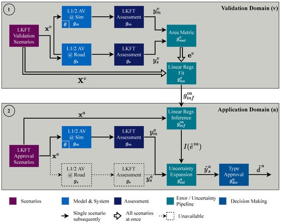
Figure 2.
Virtual-based homologation process based on previous work in ([20], Figure 1).
Both the validation and the application domain consist of several process steps, which extend from left to right in Figure 2 and are described in the following subsections. The two subsequent ones deal with the data-driven extraction of application scenarios from the simulation and the coverage-based design of validation scenarios for comparison of simulation and reality. We start with the application scenarios, since the design of the validation scenarios is directed towards them and shows methodological synergies. The actual order of scenario execution is usually inverted. The assessment subsection describes the post-processing of the results using safety measures. Subsequently, the validation results are compared and finally integrated into the actual type-approval decisions in the last two subsections in order to consider the validity of the simulation models.
3.2. Data-Driven Application Scenarios
We present a data-driven approach to extract scenarios from data that meet the requirements of the regulation. The data processing pipeline follows a rule-based algorithm:
- It partitions the scenario space into 1D acceleration bins and contiguous velocities.
- It filters the noisy lateral acceleration signal using a Butterworth filter according to [17].
- It calculates a reference lateral acceleration signal.
- It transforms the continuous time signals via thresholds to binary masks by applying condition checks.
- It merges neighboring events of ones in the masks via a connected components algorithm [60].
- It combines all binary masks using Boolean algebra.
- It extracts events from the resulting mask and represents them with start and stop time indices.
- It transforms each binary event to a scenario with mean velocity and bin-centered lateral acceleration.
We also refer to the algorithm as the event finder to highlight the data-driven condition checks. The steps of the event finder algorithm are illustrated in Figure 3 and will be explained in detail in the following. This is accompanied by the respective equations to ensure the reproducability of this paper. We define symbols for the scenario and assessment quantities of Section 3.2, Section 3.3 and Section 3.4 inspired by their written names. The longitudinal velocity is called , the lateral acceleration , the road radius r, the curvature , the lateral distance to line y, the time t, a binary mask b and the lower and upper acceleration ranges and . Further indices are required to make distinctions. Vectors are denoted as bold symbols and matrices as upper case letters.

Figure 3.
Data-driven condition checks and assessment at the exemplary application scenario and . The continuous signals in (a) are inputs to the conditions checks, whereas the binary signals in (b) are its outputs. The signals shown in (c) refer to the distance of the vehicle edges to the left and right lane markings and their minimum value over time. For decision making, we only consider the global minimum highlighted in red.
In the first step, we partition the lateral acceleration dimension into stationary interval ranges (bins) with
consisting of 10% steps of in the manner of R-79. We dispense with an analog partitioning into velocity bins, since it can be set very precisely in the experiment. Figure 3a contains the lateral acceleration signal of the vehicle after applying the Butterworth filter of the second step and the “necessary lateral acceleration to follow the curve” [4]. We refer to the latter as reference lateral acceleration
In contrast to the former, it is not based on the vehicle trajectory, but on the road radius r and curvature from maps. We aggregate all time steps in vectors and denote them as bold symbols, for example, with time steps. Figure 3b contains multiple binary mask signals from the fourth processing step. The velocity mask
is derived by comparing the velocity signal with the lower and upper velocity limits and from the vehicle manufacturer. Multiple lateral acceleration masks
are derived by checking whether the acceleration signal lies within the stationary interval ranges . In the fifth step, we apply the connected components algorithm to pull-up short gaps between separated islands in the acceleration masks to get the updated masks . According to the proposed amendment [17], the gaps may be up to 2 s if the additional condition
is fulfilled. Combining all masks with a logical AND-operator yields the resulting masks
In the seventh step, we extract all events from the entire data set whose duration is larger than the threshold . Each event j is characterized by its start time step and its end time step . We represent the scalar velocity parameter as the mean value during the start and end time steps and the acceleration parameter as the center of the selected bin:
After presenting the rule-based algorithm, we select a data set for the proof of concept. We take the same road network—with selected curve sections of the German roads A7 and B19—as prepared anyway according to the coverage-based algorithm of the following subsection. However, we let the virtual vehicle drive the route several times at arbitrary speeds instead of predefining them according to a special pattern. Figure 4 shows the resulting application scenarios. They are positioned in the center of the acceleration bins and their velocities are distributed contiguously. The distribution of points is random due to the velocities and will be discussed in the results section in more detail.
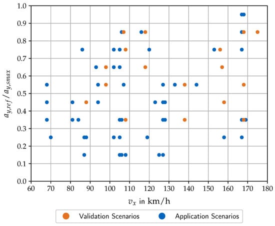
Figure 4.
Coverage-based validation scenarios and data-driven application scenarios. The 2D grid cells are used by the coverage-based algorithm. The data-driven algorithm uses only the acceleration grid and has contiguous velocities with a maximum resolution of 1/.
3.3. Coverage-Based Validation Scenarios
After the extraction of application scenarios in the last section, the focus is now on the generation of coverage-based validation scenarios. The approach uses both the requirements of the regulation with regard to the scenario conditions as well as road maps with radius r and curvature information. The coverage-based algorithm consists of the following steps:
- It partitions the velocity and acceleration dimension into 1D bins and the scenario space into 2D bins.
- It takes full-factorial samples within each velocity bin.
- It calculates a reference lateral acceleration signal across the entire road for each velocity sample.
- It transforms the continuous signals into binary masks by comparison with the acceleration bins.
- It merges neighboring events of ones in the masks via a connected components algorithm [60].
- It combines all binary masks using Boolean algebra.
- It extracts events from the binary masks and represents them with start and stop time indices.
- It selects the longest event for each 2D bin over all velocity samples and all road curves.
- We manually select single 2D bins based on the event length and a coverage criterion.
- It represents each selected 2D bin with its center as scenario parameters.
The steps of the coverage-based algorithm will be explained in detail in the following. The width of the velocity bins is 10 / and the width of the acceleration bins is 10% of . We distinguish combined 2D bins and separate 1D bins of both scenario parameters. We take 10 full-factorial samples within each velocity bin to get several velocities . In the third step, combining the radius information from the road maps with the sampled velocities yields several reference lateral acceleration signals . The steps 4–7 are similar to the steps 4–7 from the data-driven algorithm. To avoid repetition, we refer back to the previous descriptions at this point. Due to the extension to 2D bins, we get three indices of the acceleration bin, the velocity bin and the event number within the bin and ultimately the start and stop time steps and of each event. The eighth step reduces the amount of events by performing a maximum operation
over the event duration to use only the longest event per bin with the final duration . In addition, we manually reduce the number of events by selecting individual bins that excel with a high event length and a good coverage of the entire scenario space. A coverage-based design of validation scenarios can be seen in Figure 4. The coordinates of the scenario points result from the final tenth step that represents each selected bin with its coordinate center. The distribution of points results from the availability of curves in the used segments of the German roads A7 and B19 and will be discussed in the results section in more detail. An exemplary scenario is projected on the corresponding road section in Figure 5. Each validation scenario will be repeated several times to get information about the reproducibility of the real and virtual (hybrid) experiments and to be able to apply statistical validation metrics. According to [24], we will generally use at least three repetitions if possible and ten to fifteen repetitions for individual scenarios for a detailed analysis.

Figure 5.
Vehicle trajectories from an exemplary real test drive (Road) and a simulation (Sim) at the validation scenario and , located on a OpenStreetMap of the German motorway A7. These trajectories of the vehicle’s center of gravity are shown at this point for illustration purposes, but not to derive detailed distances from the vehicle edges to the lines.
If only larger measurement files can be stored after the tests have been carried out, it is possible to use data-based techniques in post-processing to locate the planned coverage-based scenarios. On the one hand, the measured vehicle coordinates can be compared with the coordinates of the planned scenarios on the map. On the other hand, the data-driven pipeline from Section 3.2 can be adapted by using, for example, the planned acceleration bins as predefined ranges in Equation (5).
3.4. Assessment
So far, the two scalar parameters and characterize the coverage-based validation scenarios and the data-driven application scenarios. The subsequent framework block called assessment deals with the lane-keeping behavior as output of the AV in dependence of both scenario parameters as inputs to the AV. According to the regulation, the behavior is characterized by the distance to line. Similar to the scenario parameters, we represent the distance to line via a Key Performance Indicator (KPI). Since we are interested in any lane crossing, we extract the minimum distance to line as worst-case behavior from a safety perspective according to Figure 3c. If even the minimum value is greater than zero, the entire trajectory (including the outer vehicle edges) will not cross the lane. In the first step, we take the minimum value of both the distance to left line signal
and analogously the distance to right line signal during the time interval of the j-th event. In the second step, we combine both minima to an overall minimum
in order to get one representative safety KPI for a consistent illustration in this paper. In summary, the behavior of the AV can be described as the mapping
from the scenario parameters to the distance KPI.
The scenario parameters can also be combined to the input vector to get a compact notation for the remaining sections and to ensure consistency with our previous paper [20]. Each coverage-based validation scenario yields for both the simulation model and the physical system a minimum distance to line and , respectively. Similarly, each application scenario provides a minimum distance to line for the simulation . In addition, we aggregate all validation scenarios into the matrix and all application scenarios into the matrix . The respective symbols are summarized in the framework in Figure 2 for a central overview. Regarding the validation domain, we require an additional notation for the measurement repetitions of the same validation scenario . All minimum distances along the repetition dimension are represented in the form of an Empirical Cumulative Distribution Function (ECDF) . The number of test repetitions determines the number of ECDF steps and varies between different scenarios and both test environments.
3.5. Model Validation
After the assessment in the validation domain, the validation metric operator quantifies the difference between the minimum distance to line from the physical system on the road and from the simulation model . One option would be to average over the test repetitions and then calculate the distance between the two averaged values. However, we decide against this validation metric, because averaging causes a loss of information. Instead, we calculate the area between the whole ECDFs. There are three possibilities for each validation scenario. Either the ECDF of the simulation lies completely on the left-hand side of the system ECDF, completely on the right-hand side, or both intersect. The first case is most critical from a safety perspective, as the simulation suggests safer behavior than would be the case in reality. Whereas the first case yields only a left area (and zero right area) and the second case only a right area (and zero left area), the third case yields a separate left and right area
This occurs when simulation and measurement show a desired similar behavior, but the simulation typically has less scatter, so that its steeper ECDF crosses the flatter one of the system. The principle of two areas is visualized in Figure 6 for one scenario.

Figure 6.
Area validation metric at the exemplary validation scenario and . The left and right areas refer to the perspective of the model with the system on its left or right side.
Thus, calculating the validation metric for all the validation scenarios yields two vectors and for the left and right areas of the minimum distance to line. We aggregate this knowledge about the validity of the simulation in an error model in order to be able to infer it to new scenarios in the application domain. This is particularly important because it is risky to compare the deviations only with the permissible tolerances, but to neglect them if they are considered suitable. These modeling errors can lead to wrong type-approval decisions regarding the safety of the vehicle and ultimately to accidents in the real world. We use a multiple linear regression model based on ([28], p. 657) to model the left area
and the right area, respectively. The hat symbol emphasizes that the error model result is an estimation from validation to application scenarios. The regression weights are calculated using a least square optimization with the validation metric results as training data.
Since the error model itself is not perfect, it remains a mean squared error s when comparing the estimations with the training data at the validation scenarios. This mean squared error and a t-distribution with a confidence of can be used to calculate a non-simultaneous Bonferroni-type prediction interval function ([61], p. 115)
The prediction interval (PI) contains the uncertainty of the error model—as does a confidence interval—and additionally the uncertainty associated with the prediction to an unseen application scenario . Thus, both the regression estimate and the PI predict from validation to application scenarios. Combining the regression estimate with the upper bound of the PI for both the left and right area finally yields the modeling uncertainty interval
with the left and right interval limits, denoted and . It can be seen as a statistical statement that the unknown true error at unseen application scenarios
lies with a high probability within those epistemic bounds [28].
3.6. Type Approval
This subsection combines the assessment results of the simulation at the data-driven application scenarios from Section 3.2 with the estimated model uncertainties from the preceding subsection. It treats each application scenario individually, since there are no test repetitions compared to the coverage-based validation experiments. We use the uncertainties to expand the minimum distance to line to an interval-valued prediction
of the unknown true minimum distance to line from the real vehicle. As shown in Figure 7, the lower bound of the left area metric estimate shifts the nominal simulation result to the left, and the upper bound of the right area metric estimate shifts it to the right. It is important to note that we use this interval prediction including uncertainties for type approval instead of the nominal simulation results, which are imperfect by the nature of the inherent models.
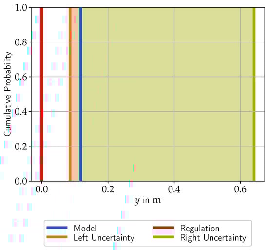
Figure 7.
Type approval at the exemplary application scenario and . The shift to the left results from the error model of the left area metric, parameterized over all validation scenarios and inferred to this application scenario, plus its prediction interval. The shift to the right results analogously from the right error model and its prediction interval.
In the end, the minimum distance to line must exceed the threshold of zero to pass the type approval. In the exemplary application scenario in Figure 7, this is the case for both the nominal simulation and more importantly for the interval-valued prediction, including the estimated model uncertainties. Figuratively speaking, exceeding the threshold value means that the outer edges of the vehicle plus a buffer for the modeling errors do not cross the lane markings. Since the distance requirement has only a lower threshold and since we defined the minimum distance as the minimum over the left and right distances in Section 3.4, we must only look at the lower bound and the left edge of from a worst case safety point of view. Nevertheless, the methodology works in analogy for quantities with upper thresholds.
4. Results and Discussion
This section presents and discusses the results for the exemplary R-79 LKFT use case based on the described methodology. The structure of the section is similar to the preceding one. It starts again with the data-driven extraction of application scenarios and the coverage-based generation of validation scenarios. Subsequently, it focuses on the model validation and type-approval results. Whereas we illustrated the methodology with examples of individual scenario points, this section aims to gain knowledge about the entire scenario space.
4.1. Data-Driven Application
This subsection begins with a pre-analysis of the minimum required event length to parameterize the event finder. The longer the minimum length is, the more meaningful the events are, but the fewer are found. Therefore, we investigate the number of extracted events, their duration and their coverage of the scenario space for varying values of the minimum length hyperparameter and select as a reasonable trade-off. After the data-driven extraction of application scenarios, the shortest event has a duration of , the longest event of and the average event of . The distribution of the data-driven application scenarios is shown in Figure 4. As desired, it contains randomness to generate unforeseen test scenarios for type approval that do not follow a predefined pattern. The rule-based algorithm extracts 62 application scenarios from the road data set. The latter is reused from the coverage-based scenario design and consists of selected curves from the German roads A7 and B19 and connecting straight sections in between. This exploits the efficiency advantage of the virtual environment. Since the length of the road data set is , this corresponds to a frequency of 0.88 events per kilometer. Due to the randomness in the scenario distribution, the granularity of the points varies across the scenario space and includes small holes. Nevertheless, the distribution and amount of scenarios is suitable for a first proof of concept.
4.2. Coverage-Based Validation Scenarios
The coverage-based validation scenarios are based on an offline scenario design that has to be executed afterwards at the real road and the virtual environment. Therefore, it is important to analyze whether there are significant deviations between the planned and observed conditions. After the test execution, we used the data-driven event finder to check whether the measured velocity and the calculated reference lateral acceleration matches the planned bin. Due to oscillations in the curvature of the real road and in the velocity, a couple of test repetitions were lost due to the condition checks. Nevertheless, the coverage-based design was accurate enough to preserve all distinct validation scenarios with at least two repetitions and in some scenarios with more than ten repetitions. This fits to the recommendation by [24] as described in Section 3.3. The number of validation scenarios is smaller than the number of application scenarios to legitimize the model-based process. The distribution of validation scenarios is shown in Figure 4. It is selected based on maximizing both scenario coverage and scenario duration to obtain representative and reproducible scenarios for a fair comparison between simulation and reality. The scenarios are distributed across the entire space with small holes in between and with gaps at the edges at low velocities and low lateral accelerations. The validation methodology including prediction intervals should be capable of dealing with this degree of interpolation and extrapolation.
Furthermore, we analyze the reproducability of the hybrid test environment including hardware components. There are many factors that have an influence on the repetitions, such as the scenario environment and the localization of the event within the measurement files by using the event finder. We illustrate the reproducability analysis in this paper both with a qualitative comparison of time series and histogram data in Figure 8, as well as with quantitative measures in Table 1. The similarity of the time signals in general and the similarity in characteristic points like minima and maxima is clearly recognizable. This demonstrates that the localization works accurately and the lateral driving behavior correlates between repetitions. The distribution of the lateral acceleration in the histogram shows narrow bands in the order of magnitude of the bins from the scenario design. The similar values of the quantitative measures mean value, standard deviation and variance reinforce the qualitative statements.
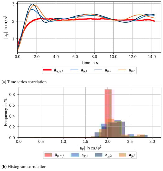
Figure 8.
Correlation analysis with (a) time series and (b) derived histogram data (15 bins). On the one hand, both subplots contain the lateral acceleration signals of three repetitions. On the other hand, they contain the averaged reference lateral acceleration signal , as the three repetitions almost coincide. The peaks at the beginning of the signals are caused by the transient passage between the straight line and the curve entrance at the validation scenario and .

Table 1.
Correlation analysis with statistical measures.
4.3. Assessment
The preceding subsection have already indicated that there is a correlation of the scenario conditions across several test repetitions. This subsection goes two steps further by looking at the assessment results and by performing an analysis across the entire scenario space. Figure 9 shows a surface plot with uncertainty bands for both the (hybrid) simulation in Figure 9a and the real world in Figure 9b. It includes both the scatter due to the test repetitions by means of vertical lines and the trend across the entire scenario space by plotting the mean value of all repetitions as the surface. At first, we look at the length of the vertical lines to analyze the repeatability. Both plots include scatter due to the complexity of the prototype vehicle, the testing environments and the scenarios. The scatter of the simulation is on average of the same order of magnitude as in reality. Despite the scatter, each mean surface indicates a clear tendency. Higher lateral accelerations and higher velocities for constant curve radii lead to smaller distance to lines. This meets the expectations for a characteristic cornering behavior. Both test environments include scenario points with a distance to line of zero corresponding to a fail of the requirements in the type approval later. The relative orientation of both surfaces is decisive for model validation in the following subsection. The surface of the simulation is flatter and lower, thus showing a significantly worse behavior of the lane-keeping assist in the virtual world. This is already an important finding of the presented methodology that is used by the developers of the virtual environment to enhance its maturity.

Figure 9.
Minimum distance to line across all validation scenarios. Each dot represents a test repetition, each line the scatter across the repetitions and the entire surface the mean value of the repetitions interpolated across the scenario space. The colors of the vertical lines are used for differentiation. They have no meaning in terms of content.
4.4. Model Validation
For the comparison between the assessment results from simulation and real driving, we use the area validation metric described in Section 3.5 and illustrated in Figure 6 for one validation scenario. Performing the same area calculations for all coverage-based validation scenarios yields the left and right error vectors and . The left error values are highlighted as points in Figure 10. Most points are zero indicating that the entire system ECDF lies on the left side of the simulation ECDF. The highest value is located at (see Figure 6). The right error counterparts are not visualized due to limited space. They lie mostly in the range between 0.1 –0.3 . Thus, the validation metric successfully quantifies the findings from the previous subsection showing smaller distances to line for the simulation compared to real driving.
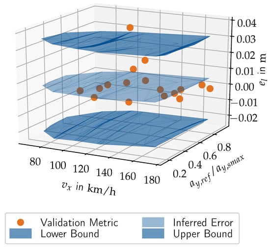
Figure 10.
Validation errors, error regression estimates and additional prediction intervals.
The left errors are used to parameterize the corresponding left linear regression model. It is visualized as the central response surface in Figure 10 across the entire application space. It reflects the horizontal trend of the left error points. It is certainly not possible and desired to match all points exactly, since they include some scatter. Therefore, we introduced the prediction intervals that cover the uncertainties of regression and prediction to the unseen application scenarios. These intervals are visualized as additional response surfaces for a statistical confidence of . They manage to bound the error points for all validation scenarios except one. In the case of the visualized small left errors, the effect is almost negligible. However, in the case of the larger right errors with significant scattering, the prediction uncertainty adds on average another resulting in a range between 0.3 –0.5 .
4.5. Type Approval
The type-approval decision making is shown in Figure 7 for an exemplary application scenario. Both the nominal simulation and the one including the modeling errors are passing the regulation threshold of zero distance to line. However, in many cases the distance to line of the simulation is relatively small. Figure 11 contains the binary pass/fail decisions across all data-driven application scenarios. In 30 out of the 62 scenarios the simulation passes the type approval, in 32 out of the 62 it fails. Since the left modeling errors—relevant from the safety perspective—were negligibly small, the decisions of the nominal simulation and the one including the uncertainties are identical for all scenarios except one. The passed scenarios show that the lane-keeping assist successfully masters many situations in this complex test environment. Nevertheless, from a safety perspective, there is a big gap left to master all situations.
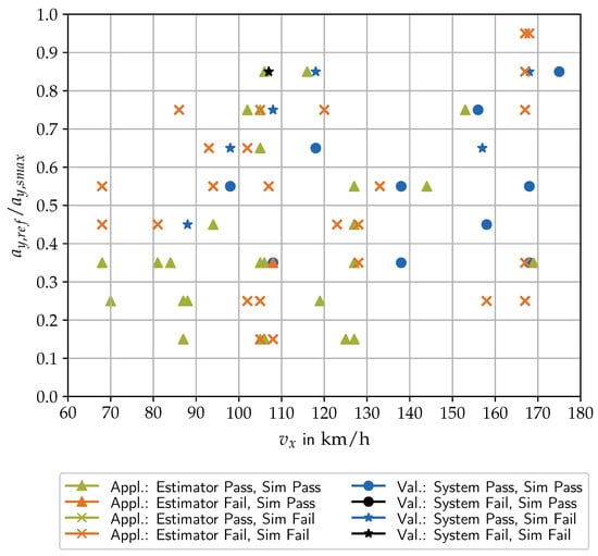
Figure 11.
Type-approval decisions at all application scenarios for the nominal simulation (Sim) and for the error estimator and at all validation scenarios for the simulation and the real system.
We extend the analysis to investigate individual factors leading to the results. The validation methodology already found that the simulation shows smaller distances to line compared to reality. This insight is already being used by the developers of the virtual environment to reduce the modeling errors, so that the number of unjustified failed cases is significantly reduced. In addition, Figure 11 reuses the validation results from Figure 9 for type approval to obtain further pass/fail decisions of the simulation, and in particular of the real system. Since the validation scenarios include repetitions leading to several ECDF steps, we can specify a confidence of decision making based on the granularity of the steps. We select a fixed confidence of resulting from two repetitions as the lowest number of repetitions across all validation experiments. This corresponds to a true decision for an entire scenario if at least half of the repetitions pass. This confidence is suitable for ensuring comparability between validation scenarios with repetitions and application scenarios without repetitions. However, it should be increased from a purely safety point of view, as shown at the end of this paragraph. The simulation shows a ratio of 10 passed to 7 failed cases. This indicates that the behavior of the simulation is safer for the coverage-based validation scenarios than for the data-driven application scenarios. The reason is that the lane-keeping assist is an ADAS not designed to drive without driver cooperation during longer data-driven routes. Nevertheless, our focus is on the development of methods with a view to higher automation levels anyway. Finally, we analyze the vehicle behavior in the real world across all validation scenarios. For a confidence of , the real vehicle passes in 16 out of the 17 cases. Taking a closer look at the repetitions of each validation scenario (see Figure 9b), shows that further failed cases exist when increasing the confidence.
In summary, the real vehicle drives more centered compared to the virtual environment, but still not centered enough in all scenarios so that individual fails occur. There are two main possibilities to improve the results in the future. On the one hand, the driving behavior of the controller can be more strongly adjusted for safety, so that it adds safety buffers and avoids lane crossings. On the other hand, the modeling errors and uncertainties of the simulation can be reduced compared to reality.
5. Conclusions
For credible type approval of automated vehicles based on simulations, an overall process is essential that not only assesses the safety of the vehicle, but also the quality of the models. We presented the corresponding validation and assessment methodology in this paper using the exemplary type approval of a vehicle’s lane-keeping behavior. At first, we focused on coverage-based and data-driven scenario design techniques that are capable of dealing with the complexity of real-world effects. Afterwards, we quantified the modeling errors and uncertainties of the simulation, represented them in the form of a data-driven error model and evaluated the vehicle behavior compared to the type-approval requirements considering these estimated errors.
The coverage-based validation scenarios were planned based on actual map data. Of course, some real-world artifacts compared to the initial planning such as noisy signals occurred. Nevertheless, a data-driven post-processing was mostly able to localize the theory within the real signals. In the future, it will be possible to integrate further map information such as the road profile and vehicle parameters to further improve the planning accuracy. Analyzing the lane-keeping behavior across all scenarios results in a clear and realistic tendency of lower distances to line at higher accelerations despite the scatter. The choice of the coverage-based approach for model validation has been rewarded, because it allows running multiple test repetitions for a fair comparison between real road and simulation. The data-driven approach is able to identify many application scenarios with low effort of cost and time. The distribution of the scenario points is both random and realistic due to the selection of actual map data. The identified data-driven scenarios show a good coverage of the application scenario space.
The validation methodology identified that both test environments show the same trend on average, but also that there are deviations between simulation and reality. Measures are currently taken by the developers of the virtual environment to reduce the modeling errors. In half of the application scenarios it can be shown that the simulation still passes the type approval, although the estimated uncertainties have been added as additional guarantees. The vehicle on the real road passes most of the scenarios, but also fails in individual ones. Therefore, it is advisable to choose a more centered trajectory with more safety buffers. Then, failed type-approval decisions can be avoided and in the future even further uncertainties of scenario and vehicle parameters can be considered to increase the statistical guarantees. It is of further interest to extend the use case from the quasi-stationary lane keeping tests on the highway to higher automation levels and operational design domains.
Author Contributions
S.R. and D.S. contributed equally to this publication. S.R. initiated this work and wrote a large part of it. D.S. developed the coverage-based and data-driven scenario methods. S.R. improved and formalized them and developed the presented validation and homologation methodology. D.S. was responsible for the data acquisition. Both S.R. and D.S. wrote the corresponding software parts, brought them together and improved the results in many joint discussions. D.W., F.D. and B.S. contributed to the conception of the research project and revised the paper critically for important intellectual content. F.D. gave final approval of the version to be published and agrees to all aspects of the work. As a guarantor, he accepts responsibility for the overall integrity of the paper. All authors have read and agreed to the published version of the manuscript.
Funding
The research project was funded and supported by TÜV SÜD Auto Service GmbH.
Institutional Review Board Statement
Not applicable.
Informed Consent Statement
Not applicable.
Data Availability Statement
Data sharing is not applicable to this article.
Acknowledgments
The authors want to thank TÜV SÜD Auto Service GmbH for the support and funding of this work. Additionally, the authors want to thank Tobias Tarne and Paul Weiner for their contributions during the test execution. Further thanks to Thomas Ponn for proofreading the article and for enhancing the content due to his critical remarks.
Conflicts of Interest
The authors declare no conflict of interest.
References
- World Health Organization. Global Status Report on Road Safety 2018; WHO: Geneva, Switzerland, 2018. [Google Scholar]
- SAE International. SAE J3016: Taxonomy and Definitions for Terms Related to Driving Automation Systems for On-Road Motor Vehicles; SAE: Warrendale, PA, USA, 2018. [Google Scholar]
- European Commission. Road Safety: Commission Welcomes Agreement on New EU Rules to Help Save Lives; European Commission: Brussels, Belgium, 2019. [Google Scholar]
- United Nations Economic Commission for Europe (UNECE). Addendum 78: UN Regulation No. 79—Uniform Provisions Concerning the Approval of Vehicles with Regard to Steering Equipment; UNECE: Geneva, Switzerland, 2018. [Google Scholar]
- United Nations Economic Commission for Europe (UNECE). Proposal for a New UN Regulation on Uniform Provisions Concerning the Approval of Vehicles with Regards to Automated Lane Keeping System (ECE/TRANS/WP.29/2020/81); UNECE: Geneva, Switzerland, 2020. [Google Scholar]
- German Aerospace Center. PEGASUS-Project; German Aerospace Center: Cologne, Germany, 2019. [Google Scholar]
- Leitner, A.; Akkermann, A.; Hjøllo, B.Å.; Wirtz, B.; Nickovic, D.; Möhlmann, E.; Holzer, H.; van der Voet, J.; Niehaus, J.; Sarrazin, M.; et al. ENABLE-S3: Testing & Validation of Highly Automated Systems: Summary of Results; Springer: Berlin, Germany, 2019. [Google Scholar]
- Kalra, N.; Paddock, S.M. Driving to safety: How many miles of driving would it take to demonstrate autonomous vehicle reliability? Transp. Res. Part A Policy Pract. 2016, 94, 182–193. [Google Scholar] [CrossRef]
- Bagschik, G.; Menzel, T.; Maurer, M. Ontology based Scene Creation for the Development of Automated Vehicles. In Proceedings of the 2018 IEEE Intelligent Vehicles Symposium (IV), Changshu, China, 26–30 June 2018; pp. 1813–1820. [Google Scholar] [CrossRef]
- Langner, J.; Bach, J.; Ries, L.; Otten, S.; Holzäpfel, M.; Sax, E. Estimating the Uniqueness of Test Scenarios derived from Recorded Real-World-Driving-Data using Autoencoders. In Proceedings of the 2018 IEEE Intelligent Vehicles Symposium (IV), Changshu, China, 26–30 June 2018; pp. 1860–1866. [Google Scholar]
- Krajewski, R.; Moers, T.; Nerger, D.; Eckstein, L. Data-Driven Maneuver Modeling using Generative Adversarial Networks and Variational Autoencoders for Safety Validation of Highly Automated Vehicles. In Proceedings of the 2018 IEEE 21th International Conference on Intelligent Transportation Systems (ITSC), Maui, HI, USA, 4–7 November 2018; pp. 2383–2390. [Google Scholar]
- Althoff, M.; Dolan, J.M. Reachability computation of low-order models for the safety verification of high-order road vehicle models. In Proceedings of the 2012 American Control Conference (ACC), Montreal, QC, Canada, 27–29 June 2012; pp. 3559–3566. [Google Scholar]
- Beglerovic, H.; Ravi, A.; Wikström, N.; Koegeler, H.M.; Leitner, A.; Holzinger, J. Model-based safety validation of the automated driving function highway pilot. In 8th International Munich Chassis Symposium 2017; Pfeffer, P.E., Ed.; Springer Fachmedien Wiesbaden: Wiesbaden, Germany, 2017; pp. 309–329. [Google Scholar]
- Riedmaier, S.; Ponn, T.; Ludwig, D.; Schick, B.; Diermeyer, F. Survey on Scenario-Based Safety Assessment of Automated Vehicles. IEEE Access 2020, 8, 87456–87477. [Google Scholar] [CrossRef]
- United Nations Economic Commission for Europe (UNECE). Addendum 139—Regulation No. 140—Uniform Provisions Concerning the Approval of Passenger Cars with Regard to Electronic Stability Control (ESC) Systems; UNECE: Geneva, Switzerland, 2017. [Google Scholar]
- Lutz, A.; Schick, B.; Holzmann, H.; Kochem, M.; Meyer-Tuve, H.; Lange, O.; Mao, Y.; Tosolin, G. Simulation methods supporting homologation of Electronic Stability Control in vehicle variants. Veh. Syst. Dyn. 2017, 55, 1432–1497. [Google Scholar] [CrossRef]
- United Nations Economic Commission for Europe. Proposal for Amendments to ECE/TRANS/WP.29/GRVA/2019/19; UNECE: Geneva, Switzerland, 2019. [Google Scholar]
- Schneider, D.; Huber, B.; Lategahn, H.; Schick, B. Measuring method for function and quality of automated lateral control based on high-precision digital ”Ground Truth” maps. In 34. VDI/VW-Gemeinschaftstagung Fahrerassistenzsysteme und Automatisiertes Fahren 2018; VDI-Berichte; VDI Verlag GmbH: Düsseldorf, Germany, 2018; pp. 3–16. [Google Scholar]
- Keidler, S.; Schneider, D.; Haselberger, J.; Mayannavar, K.; Schick, B. Development of lane-precise “Ground Truth” maps for the objective Quality Assessment of automated driving functions. In Proceedings of the 17 Internationale VDI-Fachtagung Reifen—Fahrwerk—Fahrbahn, Düsseldorf, Germany, 16–17 October 2019. [Google Scholar]
- Riedmaier, S.; Danquah, B.; Schick, B.; Diermeyer, F. Unified Framework and Survey for Model Verification, Validation and Uncertainty Quantification. Arch. Comput. Methods Eng. 2020. [Google Scholar] [CrossRef]
- Rosenberger, P.; Holder, M.; Zirulnik, M.; Winner, H. Analysis of Real World Sensor Behavior for Rising Fidelity of Physically Based Lidar Sensor Models. In Proceedings of the 2018 IEEE Intelligent Vehicles Symposium (IV), Changshu, China, 26–30 June 2018; pp. 611–616. [Google Scholar]
- Schaermann, A.; Rauch, A.; Hirsenkorn, N.; Hanke, T.; Rasshofer, R.; Biebl, E. Validation of vehicle environment sensor models. In Proceedings of the 2017 IEEE Intelligent Vehicles Symposium (IV), Los Angeles, CA, USA, 11–14 June 2017; pp. 405–411. [Google Scholar]
- Abbas, H.; O’Kelly, M.; Rodionova, A.; Mangharam, R. Safe At Any Speed: A Simulation-Based Test Harness for Autonomous Vehicles. In Proceedings of the Seventh Workshop on Design, Modeling and Evaluation of Cyber Physical Systems (CyPhy’17), Seoul, Korea, 15–20 October 2017; pp. 94–106. [Google Scholar]
- Viehof, M.; Winner, H. Research methodology for a new validation concept in vehicle dynamics. Automot. Engine Technol. 2018, 3, 21–27. [Google Scholar] [CrossRef]
- International Organization for Standardization. Passenger Cars—Validation of Vehicle Dynamic Simulation—Sine with Dwell Stability Control Testing; ISO: Geneva, Switzerland, 2016. [Google Scholar]
- Riedmaier, S.; Nesensohn, J.; Gutenkunst, C.; Düser, T.; Schick, B.; Abdellatif, H. Validation of X-in-the-Loop Approaches for Virtual Homologation of Automated Driving Functions. In Proceedings of the 11th Graz Symposium Virtual Vehicle (GSVF), Graz, Austria, 15–16 May 2018; pp. 1–12. [Google Scholar]
- Groh, K.; Wagner, S.; Kuehbeck, T.; Knoll, A. Simulation and Its Contribution to Evaluate Highly Automated Driving Functions. In WCX SAE World Congress Experience; SAE Technical Paper Series; SAE International400 Commonwealth Drive: Warrendale, PA, USA, 2019; pp. 1–11. [Google Scholar]
- Oberkampf, W.L.; Roy, C.J. Verification and Validation in Scientific Computing; Cambridge University Press: Cambridge, UK, 2010. [Google Scholar]
- Ao, D.; Hu, Z.; Mahadevan, S. Dynamics Model Validation Using Time-Domain Metrics. J. Verif. Valid. Uncertain. Quantif. 2017, 2, 011004. [Google Scholar] [CrossRef]
- Voyles, I.T.; Roy, C.J. Evaluation of Model Validation Techniques in the Presence of Aleatory and Epistemic Input Uncertainties. In Proceedings of the 17th AIAA Non-Deterministic Approaches Conference, Kissimmee, FL, USA, 5–9 January 2015; American Institute of Aeronautics and Astronautics: College Park, MD, USA, 2015; pp. 1–16. [Google Scholar]
- Kennedy, M.C.; O’Hagan, A. Bayesian calibration of computer models. J. R. Stat. Soc. Ser. B 2001, 63, 425–464. [Google Scholar] [CrossRef]
- Sankararaman, S.; Mahadevan, S. Integration of model verification, validation, and calibration for uncertainty quantification in engineering systems. Reliab. Eng. Syst. Saf. 2015, 138, 194–209. [Google Scholar] [CrossRef]
- Hills, R.G. Roll-Up of Validation Results to a Target Application; Sandia National Laboratories: Albuquerque, NM, USA, 2013.
- Mullins, J.; Schroeder, B.; Hills, R.; Crespo, L. A Survey of Methods for Integration of Uncertainty and Model Form Error in Prediction; Probabilistic Mechanics & Reliability Conference (PMC): Albuquerque, NM, USA, 2016. [Google Scholar]
- Schuldt, F.; Menzel, T.; Maurer, M. Eine Methode für Die Zuordnung Von Testfällen für Automatisierte Fahrfunktionen auf X-In-The-Loop Simulationen im Modularen Virtuellen Testbaukasten; Workshop Fahrerassistenzsysteme: Garching, Germany, 2015; pp. 1–12. [Google Scholar]
- Böde, E.; Büker, M.; Ulrich, E.; Fränzle, M.; Gerwinn, S.; Kramer, B. Efficient Splitting of Test and Simulation Cases for the Verification of Highly Automated Driving Functions. In Computer Safety, Reliability, and Security; Gallina, B., Skavhaug, A., Bitsch, F., Eds.; Springer International Publishing: Cham, Switzerland, 2018; pp. 139–153. [Google Scholar]
- Morrison, R.E.; Bryant, C.M.; Terejanu, G.; Prudhomme, S.; Miki, K. Data partition methodology for validation of predictive models. Comput. Math. Appl. 2013, 66, 2114–2125. [Google Scholar] [CrossRef]
- Terejanu, G. Predictive Validation of Dispersion Models Using a Data Partitioning Methodology. In Model Validation and Uncertainty Quantification, Volume 3; Atamturktur, H.S., Moaveni, B., Papadimitriou, C., Schoenherr, T., Eds.; Springer International Publishing: Cham, Switzerland, 2015; pp. 151–156. [Google Scholar]
- Mullins, J.; Mahadevan, S.; Urbina, A. Optimal Test Selection for Prediction Uncertainty Reduction. J. Verif. Valid. Uncertain. Quantif. 2016, 1. [Google Scholar] [CrossRef]
- Forschungsgesellschaft für Straßen- und Verkehrswesen. Richtlinien für die Anlage von Autobahnen; FGSV: Cologne, Germany, 2008. [Google Scholar]
- Chen, W.; Kloul, L. An Ontology-based Approach to Generate the Advanced Driver Assistance Use Cases of Highway Traffic. In Proceedings of the 10th International Joint Conference on Knowledge Discovery, Knowledge Engineering and Knowledge Management, Seville, Spain, 18–20 September 2018; pp. 1–10. [Google Scholar]
- Li, Y.; Tao, J.; Wotawa, F. Ontology-based test generation for automated and autonomous driving functions. Inf. Softw. Technol. 2020, 117, 106200. [Google Scholar] [CrossRef]
- Beglerovic, H.; Schloemicher, T.; Metzner, S.; Horn, M. Deep Learning Applied to Scenario Classification for Lane-Keep-Assist Systems. Appl. Sci. 2018, 8, 2590. [Google Scholar] [CrossRef]
- Gruner, R.; Henzler, P.; Hinz, G.; Eckstein, C.; Knoll, A. Spatiotemporal representation of driving scenarios and classification using neural networks. In Proceedings of the 2017 IEEE Intelligent Vehicles Symposium (IV), Los Angeles, CA, USA, 11–17 June 2017; pp. 1782–1788. [Google Scholar]
- Kruber, F.; Wurst, J.; Morales, E.S.; Chakraborty, S.; Botsch, M. Unsupervised and Supervised Learning with the Random Forest Algorithm for Traffic Scenario Clustering and Classification. In Proceedings of the 30th IEEE Intelligent Vehicles Symposium, Paris, France, 9–12 June 2019; pp. 2463–2470. [Google Scholar]
- Wang, W.; Zhao, D. Extracting Traffic Primitives Directly From Naturalistically Logged Data for Self-Driving Applications. IEEE Robot. Autom. Lett. 2018, 3, 1223–1229. [Google Scholar] [CrossRef]
- Zhou, J.; del Re, L. Identification of critical cases of ADAS safety by FOT based parameterization of a catalogue. In Proceedings of the 2017 11th Asian Control Conference (ASCC), Gold Coast, Australia, 17–20 December 2017; pp. 453–458. [Google Scholar]
- de Gelder, E.; Paardekooper, J.P. Assessment of Automated Driving Systems using real-life scenarios. In Proceedings of the 2017 IEEE Intelligent Vehicles Symposium (IV), Los Angeles, CA, USA, 11–17 June 2017; pp. 589–594. [Google Scholar]
- Menzel, T.; Bagschik, G.; Maurer, M. Scenarios for Development, Test and Validation of Automated Vehicles. In Proceedings of the 2018 IEEE Intelligent Vehicles Symposium (IV), Changshu, China, 26–30 June 2018. [Google Scholar]
- Kim, B.; Jarandikar, A.; Shum, J.; Shiraishi, S.; Yamaura, M. The SMT-based automatic road network generation in vehicle simulation environment. In Proceedings of the 13th International Conference on Embedded Software—EMSOFT ’16, Grenoble, France, 12–16 October 2016; pp. 1–10. [Google Scholar]
- Rocklage, E.; Kraft, H.; Karatas, A.; Seewig, J. Automated scenario generation for regression testing of autonomous vehicles. In Proceedings of the 2017 IEEE 20th International Conference on Intelligent Transportation Systems (ITSC), Rhodes, Greece, 20–23 September 2017; pp. 476–483. [Google Scholar]
- Zhao, D. Accelerated Evaluation of Automated Vehicles. Ph.D. Thesis, University of Michigan, Ann Arbor, MI, USA, 2016. [Google Scholar]
- Åsljung, D.; Nilsson, J.; Fredriksson, J. Using Extreme Value Theory for Vehicle Level Safety Validation and Implications for Autonomous Vehicles. IEEE Trans. Intell. Veh. 2017, 2, 288–297. [Google Scholar] [CrossRef]
- Stark, L.; Düring, M.; Schoenawa, S.; Maschke, J.E.; Do, C.M. Quantifying Vision Zero: Crash avoidance in rural and motorway accident scenarios by combination of ACC, AEB, and LKS projected to German accident occurrence. Traffic Inj. Prev. 2019, 20, 126–132. [Google Scholar] [CrossRef] [PubMed]
- Klischat, M.; Althoff, M. Generating Critical Test Scenarios for Automated Vehicles with Evolutionary Algorithms. In Proceedings of the 2019 IEEE Intelligent Vehicles Symposium (IV), Paris, France, 9–12 June 2019; pp. 2352–2358. [Google Scholar]
- Ponn, T.; Müller, F.; Diermeyer, F. Systematic Analysis of the Sensor Coverage of Automated Vehicles Using Phenomenological Sensor Models. In Proceedings of the 2019 IEEE Intelligent Vehicles Symposium (IV), Paris, France, 9–12 June 2019; pp. 1000–1006. [Google Scholar]
- Koren, M.; Alsaif, S.; Lee, R.; Kochenderfer, M.J. Adaptive Stress Testing for Autonomous Vehicles. In Proceedings of the 2018 IEEE Intelligent Vehicles Symposium (IV), Changshu, China, 26–30 June 2018; pp. 1898–1904. [Google Scholar]
- Beglerovic, H.; Stolz, M.; Horn, M. Testing of autonomous vehicles using surrogate models and stochastic optimization. In Proceedings of the 2017 IEEE 20th International Conference on Intelligent Transportation Systems (ITSC), Yokohama, Japan, 16–19 October 2017; pp. 1–6. [Google Scholar]
- Tuncali, C.E.; Pavlic, T.P.; Fainekos, G. Utilizing S-TaLiRo as an Automatic Test Generation Framework for Autonomous Vehicles. In Proceedings of the 2016 IEEE 19th International Conference on Intelligent Transportation Systems (ITSC), Rio de Janeiro, Brazil, 1–4 November 2016; pp. 1470–1475. [Google Scholar]
- Dillencourt, M.B.; Samet, H.; Tamminen, M. A general approach to connected-component labeling for arbitrary image representations. J. ACM 1992, 39, 253–280. [Google Scholar] [CrossRef]
- Miller, R.G. Simultaneous Statistical Inference; Springer: New York, NY, USA, 1981. [Google Scholar]


Publisher’s Note: MDPI stays neutral with regard to jurisdictional claims in published maps and institutional affiliations. |
© 2020 by the authors. Licensee MDPI, Basel, Switzerland. This article is an open access article distributed under the terms and conditions of the Creative Commons Attribution (CC BY) license (http://creativecommons.org/licenses/by/4.0/).