Abstract
The mesh deformation method based on radial basis functions is widely used in computational fluid dynamics (CFD) simulation with a moving boundary. The traditional method for generating CFD mesh quality metrics called mesh-based metrics use the information of deformed mesh with specific element node coordinates and a connectivity relationship. This paper develops a new mesh quality, metric evaluating method based on the mapping process between the initial and deformed mesh, which is named mapping-based metrics. Mapping-based metrics are evaluated based on the conception of the deformation principle in continuum mechanics. This method provides a new point for mesh quality evaluation without requirements of deformed mesh coordinates and element connectivity information. Three test cases show that, comparing with indirectly solving by a geometrical method, mapping-based metrics accurately reveal the changes of the angle and area over the whole deformed domain. Additionally, the mapping-based metrics give high applicability to the quality of deformed mesh compared to mesh-based metrics. The quality evaluation method for CFD mesh proposed in this paper is effective.
1. Introduction
For computational fluid dynamics (CFD) computations and fluid-structure interaction (FSI) computations, a flows simulation with a moving boundary are often encountered at various important problems such as stability analysis of bridges, aircraft optimizations, flutter calculations, and bioengineering simulations [1,2,3,4,5]. The mesh deformation algorithm is required to adapt the CFD computational mesh with the motion of the boundary. With regards to the problems with large deformation of boundary, performance of mesh deformation methods often becomes a limiting factor to CFD simulations accuracy [6]. Meanwhile, the computational mesh needs to be updated repeatedly during an unsteady simulation, bringing large computational cost. Accuracy and computational efficiency of mesh deformation algorithm is crucial for the previously mentioned problem [7,8].
Variety of mesh deformation methods have been developed in literature in terms of accuracy, efficiency, and robustness [9]. These methods can be classified into two main categories: connectivity-based methods and node-based method. The spring analogy method [10,11] is a typical one of connectivity methods. The idea of the spring analogy method is to create a network of springs connecting all nodes in the mesh and the stiffness of springs is inversely proportional to the edge length [12]. The whole mesh can be viewed as a spring system. It has been successfully applied to many unsteady and optimization problems. However, this method is relatively expensive in computational cost due to the necessity of total mesh connectivity information, and it may lead to an invalid mesh for large deformation [13,14]. Although several strategies have been introduced to improve the ability of the spring analogy method [15,16,17], it is still difficult to guarantee both high efficiency and applicability. In the other classification of the node-based method, each node can be modified independently to its adjacent nodes, and then the deformation of mesh can be adjusted indiscriminately [12]. This method allows for large deformation and does not require connectivity information between mesh nodes. The node-based method is useful for unstructured mesh due to those characteristics. Interpolation techniques are often introduced in a node-based method. Witteveen proposed the Inverse Distance Weighed (IDW) interpolation method [18] in which the deformation of internal nodes depends on the weighted-averaging of the displacement of boundary nodes. Transfinite interpolation (TFI) developed by Gaitonode [19] is a fast scheme used in a node-based method. Despite its efficiency, the deformed mesh quality is not guaranteed, especially the orthogonality of the mesh near the boundary. Liu proposed a coarse Delaunay graph with barycentric interpolation to propagate deformation from boundary nodes to internal ones [20]. In addition, Luke et al. decreased computational cost of the previously mentioned method via tree-code optimization [21]. Although the common node-based methods increase the efficiency of generation of adapted mesh, it does not perform well with complex mesh and is not capable of preserving the mesh orthogonality.
A well-established method based on radial basis functions (RBFs) proposed by Boer [22] is a desirable approach for both structured and unstructured meshes. It can generally preserve the mesh quality with reasonable orthogonality near the boundary in mesh deformation [23]. The research shows that different RBFs introduced could result in different results [22,24,25]. Jokonsson et al. describe suggestions for choosing RBFs, and demonstrate that the computational cost will still grow as the mesh scale increases, even choosing the appropriate functions [1]. Considering the high computational cost, several approaches are proposed with greedy algorithm [21,26,27] or reducing the interpolated nodes [28,29,30]. The improved RBFs method has better computational efficiency and can also preserve the mesh quality well. Various RBFs are compared in Reference [22] and RBFs based on thin plate splines (TPS) shows good application prospects in mesh deformation, which is chosen as the mesh deformation method in this paper.
Another aspect in research of the mesh deformation algorithm is how to evaluate the quality of deformed mesh. To compare the different meshes quality after deformation, mesh quality metrics are introduced. Traditional mesh quality metrics are based on a set of Jacobian matrices, which contain information on basic element qualities such as size, orientation, shape, and skewness [22]. We assume that the initial mesh is created with an optimal quality and the elements quality should be changed as little as possible after deformation. Both the angles and volume of the elements should be preserved. Several parametric evaluation criteria have been established in the past. The relative size metrics measuring the change in element size and skew metric measuring the skewness and distortion are often used in mesh quality evaluation. Knupp proposed other typical mesh quality metrics [31] in which both the area and the angles of the element are measured. In commercial software like Pointwise [32], area ratio, aspect ratio, equiarea skewness, and equi-angle skewness are often used in mesh quality evaluation. The equiarea skewness are represented as a ratio of the mesh element area to the optimum cell area. It only applies to triangles and tetrahedral elements. The equi-angle skewness is represented as the maximum ratio of the element included angle-to-angle of an equilateral element. The angle skewness applies to all element types and is available for domains and blocks. Existing mesh quality metrics are based on specific coordinates and connectivity information of the mesh, which we called mesh-based metrics. It will lead to higher computational costs. On the other side, no attention has been paid to the quality of the mesh deformation method, which can reveal the characteristics of the deformation algorithm itself. Therefore, an efficient method that can give a criterion of the ability of the mesh deformation algorithm should be introduced.
The objective of this paper is to develop a quality metric method for unstructured and structured mesh. The RBFs mesh deformation method based on generalized TPS is introduced, and is evaluated by this metric evaluating method. Different from traditional mesh-based metrics, this quality metric method is calculated based on the mapping information between the initial and deformed mesh, so it is named mapping-based metrics in this paper. The mapping-based metrics are based on the deformation principle of continuum mechanics [33,34], which is especially suitable for nonlinear large deformation problems. Without the requirement of element connectivity information, this method possesses high efficiency.
The rest of this paper is allocated as follows. Section 2 introduces the methodology of RBFs’ mesh deformation method based on generalized TPS. Section 3 demonstrates the mapping-based metrics we proposed in detail. In Section 4, three 2-D mesh cases with structured and unstructured mesh are performed and the numerical results of the mapping-based metrics are presented. A comparison between mapping-based metrics, mesh-based metrics, and a geometric calculation directly are also been shown to illustrate the accuracy of the metrics evaluation method proposed in this paper. Finally, conclusion are described in Section 5.
2. RBFs Method Based on Generalized TPS
Radial basis functions (RBFs) interpolation can be applied to obtain the displacement of the internal fluid mesh nodes based on the deformation of the structural boundary. The basic form of RBFs interpolation can be expressed as:
where is the interpolation function, describing the displacement in the whole domain. are the centers in which the values are known. In this research, the coordinates are of the th boundary node, is the total quantity of boundary nodes, is the centers in which the values are unknown. In this research, the coordinates are of the random internal fluid mesh node, is the weight coefficient of the th RBF, is the given RBF, and represents the Euclidean distance of vector and . In 3D space, components of and are given as and , and distance has the following formulation:
The weight coefficients are determined by the interpolation conditions:
where are the actual displacements of the boundary nodes. With a matrix containing the evaluation of the basis function:
The weight coefficients vector can be obtained:
The values of internal mesh nodes displacement can be derived by calculating the interpolation Equation (1) after calculating the coefficients vector :
Where is the coordinates of the th internal mesh node.
Several RBFs can be selected in literature, which are appropriate for this research. They can be divided in two categories: compact functions and global functions [6,33]. The compact function is generally scaled with a support radius to control the compact support. The mesh nodes inside a circle (2D) or sphere (3D) with radius around a boundary node are influenced by the corresponding displacement. The global functions are not equal to zero outside a certain radius and operate on the whole interpolation space. Two categories RBFs are shown by Boer [22], and the frequency used formulations are presented in Table 1 and Table 2.

Table 1.
Radial basis functions (RBFs) with compact functions (, is the Euclidean distance and is the support radius).
Table 2.
RBFs with global functions.
We chose the thin plate spline (TPS) as the RBFs in this research, which generates the highest mesh quality of adapted mesh [25].
3. Mapping-Based Metrics
The quality of deformed mesh is evaluated by the mesh quality metrics. Most of the present research studies give quality metrics that require the topology of the initial mesh or deformed mesh. It is based on a set of Jacobian matrices containing information on mesh element qualities such as size and skewness. In this section, an efficient mesh quality metrics generation method based on a mesh deformation algorithm is introduced.
3.1. Mapping Relationships
In order to describe the motion and deformation of an element, the initial configuration is selected as the reference configuration and as the current configuration deformed. A nonsingular single-valued mapping is established, as shown in Figure 1. is set as the global coordinate system. The position of the point in the reference configuration is and its image point with the deformation process in the current configuration is . and are coordinates in . The mapping of the point can be written as:
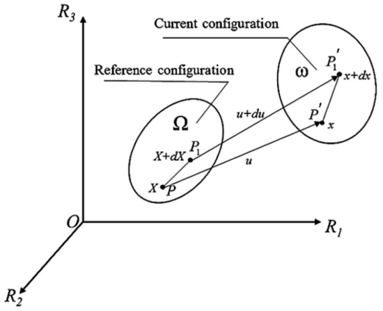
Figure 1.
Configurations in deforming the element process.
As shown in Figure 1, the position of two adjacent points in the reference configuration is given by and . The distance vector between two adjacent points is . In the current configuration, the distance vector between two adjacent points after mapping is . The transformation between and is investigated as:
where is the deformation gradient tensor.
Assuming the displacement vector of point is , then it easily follows from Equation (8) that:
Given a displacement gradient tensor , the formulation of distance can be expressed as:
It is assumed that are the unit base vectors of the reference configuration. Any vector in the reference can be expressed as . Images of unit base vectors in the current configuration is and the images of vector can be expressed as .
According to continuum mechanics [34], the relationships between coordinates of two vectors in the reference coordinates are:
Therefore, the image of the vector can be written as:
Therefore, the mapping for the vectors is:
Based on Equation (14), the coordinates of image vector according to image base vectors is the same as the coordinates of the initial vector according to initial base vectors of the reference configuration. Therefore, the mapping can be measured according to the change of unit base vectors of initial configuration over the computational domain.
Given , the length of vector can be formulated as:
The length of vector can obtained by:
According to Equation (11), it easily follows that:
where is the green strain tensor.
Equation (17) can be given in a components format by:
For a 2-D case, consider specified vectors and their image vectors . The area of the parallelogram formed by the two vectors is computed as follows:
And its image is given by:
The angle between two vectors is related to the dot product. Let be the angle between and be the angle between , then:
The mapping quality of the deformation algorithm is related to the variety of the unit base vectors in the reference configuration as mentioned before. Therefore, the mapping-based size metrics and skew metrics of the mesh deformation algorithm of a 2-D mesh are established to measure the area change and angle change based on the mapping relationship of the unit base vectors.
3.2. Size Metrics
Size metrics is to judge whether the deformed elements are too large or too small compared to the initial elements. According to Equation (20), denote as the mapping-based size metric of area change, and:
where . With deformation information, the mapping-based size metrics can be calculated with Equations (6) and (11).
means that the deformed element has the same area as the original one.
means that the deformed element is degenerate.
In a traditional method [6,22], mesh-based size metrics measuring area change could be expressed as:
where is the ratio of the area of the deformed elements to the area of the initial elements. Coordinates of each deformed and initial elements and calculation of the area are required.
3.3. Skewness Metrics
Skewness metrics is to analyse distortions of the deformed elements compared to the initial elements. According to Equation (22), denote as the mapping-based skewness metric of angle change, and:
where are items in a green strain tensor .
means that the deformed element has equal angles with the origin reference one.
means that the deformed element is degenerate.
In a traditional method [6,22], mesh-based skewness metrics, which could be also called shape metrics, could be expressed as:
The definition of variables in the expression and calculation process can be found in Reference [30]. The evaluation requires coordinates of mesh elements and determinant calculation, which brings a computational burden.
Based on the above description, the quality metrics of the generalized TPS mesh deformation algorithm used in this paper can be evaluated. The specific steps are as follows:
Step 1. Calculate the deformation of mesh nodes over the computational domain based on the RBFs method with Equation (6).
Step 2. Calculate the displacement gradient tensor according to Equation (11), based on a central difference method. With the adjacent three mesh nodes , a difference item of the central node in a displacement gradient tensor can be calculated as:
where are displacement components of the mesh node and are coordinates of the initial mesh of node .
Step 3. Calculate the green strain tensor according to Equation (17).
Step 4. Calculate the mapping-based size metrics of the mesh deformation method according to Equation (23).
Step 5. Calculate the mapping-based skewness metrics of the mesh deformation method according to Equations (25) and (26).
It should be noted that, in step 2, quality evaluation of mesh nodes on a fluid boundary is not valuable because the deformation of the fluid boundary is not clear. A difference item of boundary nodes can be equal to adjacent nodes in the fluid field inside. The mapping-based metrics only require the coordinates of initial mesh nodes and displacement of the mesh nodes as a description of step 1, which can be easily obtained from a mesh deformation process. Therefore, it can be regarded as an efficient method and can reveal the characteristic of the mesh deformation algorithm itself without information of deformed mesh.
4. Results and Discussions
In this section, three test cases have been proposed with the RBFs’ method based on generalized TPS including (1) the translation and rotation of a rectangle block with square mesh, (2) mesh deformation due to a rigid body rotation of airfoil NACA0012 with unstructured mesh, and (3) mesh transformation from airfoil NACA0012 to NACA4412 with structured mesh. Initial meshes are all generated in software Pointwise and the deformed mesh is generated by a program in C++ language. The mapping-based metrics are used to evaluate the mesh deformation algorithm. A geometrical change of elements is also measured to check the accuracy of the mapping-based metrics method proposed.
4.1. Test Case 1: Translation and Rotation of Structured Square Mesh
In the first test cases, a standard test case where the initial mesh elements are all square with a side length has been produced. As shown in Figure 2a, the computational domain has dimension and the rectangle at the center of the domain has dimension . The rectangle is rotated 45 degrees around the center. The deformed mesh based on the RBFs’ method using generalized TPS is shown in Figure 2b.
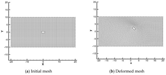
Figure 2.
Mesh of test case 1.
The mapping-based metrics proposed in this paper are used to evaluate the mesh deformation algorithm. Figure 3 shows the skewness metric and size metric over computational domain. It can be seen that the blue area is of the minimal value of quality metrics, which means the elements undergo the greatest compression and distortion over this domain.
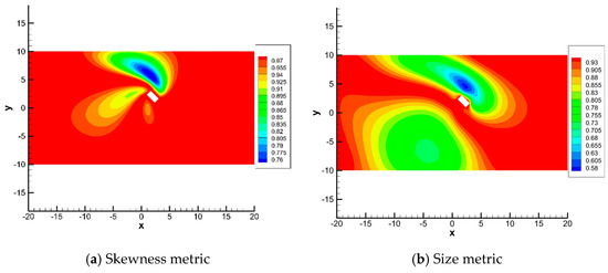
Figure 3.
Mapping-based metrics of test case 1.
The accuracy of mapping-based metrics of mesh deformation algorithm is checked using a specific element with a minimal metrics value in the blue area. Figure 4 has marked the edge of a specific element with a red line. Calculating the angle change and area ratio of a specific element, and compassion between mapping-based metrics, mesh-based metrics, and a geometrical method can be completed.
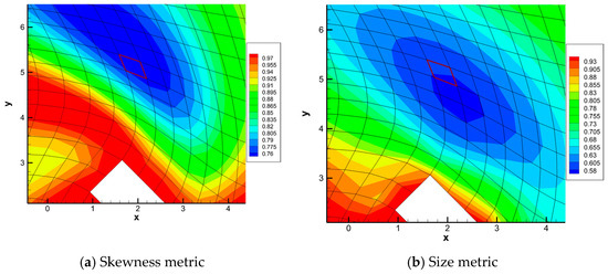
Figure 4.
Specific element with minimal metrics.
With a geometrical method, the angles of deformed mesh and area ratio from the initial mesh to deformed mesh can be calculated directly based on geometrical relationships. As quadrilateral elements, the geometrical configuration of a specific element is shown in Figure 5. The element has four nodes denoted as and is the angle between two sides joined at the th node. Calculation results of the angle change have been presented in Table 3. It can be seen that calculation results by the mapping-based metric have a very small error compared to a geometrical calculation directly, which is less than 1.5%. The area ratio calculation results of mapping-based metrics is 0.5810. It is very close to the result of the geometrical method, which has a value of 0.5803.
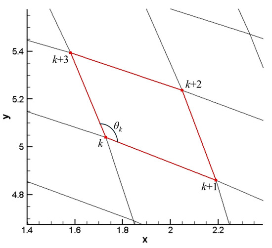
Figure 5.
Geometrical configuration of the mesh element.
Table 3.
Comparison between the mapping-based method and geometrical method.
Figure 6 shows the calculation results of traditional mesh-based metric described in Section 3.2 and Section 3.3 in this test case. The metrics distribution is nearly the same with that of mapping-based metrics presented in Figure 3. This is because every initial cell is a square, and the sides of elements are parallel to the base vectors of the initial configuration. Therefore, the changed angle between the two unit base vectors equals to the changed angle between the two sides of the deformed mesh element. Table 4 shows the comparison between two metrics and average metrics value that has also been presented. The average value of the metric over all the elements indicates the average quality of the mesh. The higher the average quality of the mesh, the more stable, accurate, and efficient the computation will be. The minimum value of the metric over all the elements indicates the quality of the cell with the lowest quality. This value is required to be larger than zero. Otherwise, the mesh will contain degenerate elements. Degenerate elements have a very negative influence on the stability and accuracy of numerical computations [22]. All the average and minimal quality metrics of size and skew calculated by mapping-based metrics and traditional mesh-based metrics methods are closed, resulting in small error values of less than 0.22%.
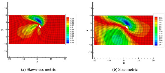
Figure 6.
Mesh-based metrics of test case 1.
Table 4.
Comparison between the mapping-based metric and mesh-based metrics.
4.2. Test Case 2: Large Rotation of NACA0012 Unstructured Mesh
This test case considers the mesh movement due to a severe rotation of airfoil NACA0012. The airfoil is initially located in the center of a circle domain with a radius of , with being the chord length of the airfoil. The trailing edge of the airfoil is initially at point and the leading edge at point . The initial mesh is triangular and given in Figure 7. Two hundred nodes on the airfoil surface and 20 nodes on the filed boundary are selected as control points to calculate RBFs’ interpolation. Control points on the airfoil surface and field boundary are presented in Figure 8.
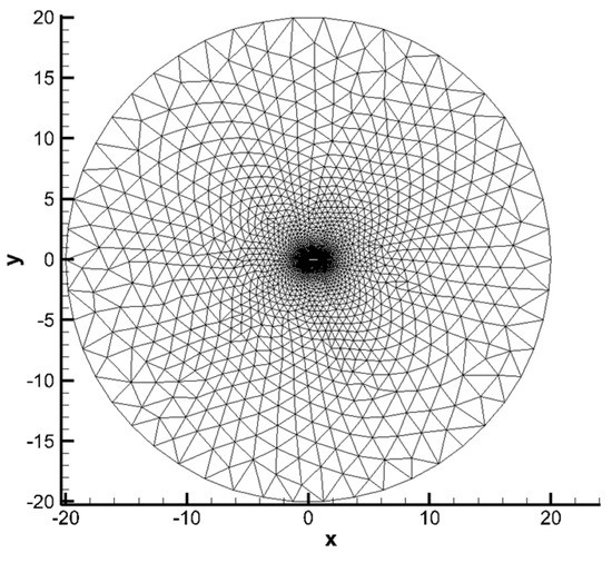
Figure 7.
Initial mesh of test case 2.
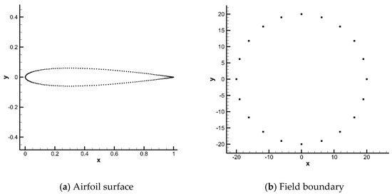
Figure 8.
Control points in test case 2.
Figure 9 shows the deformed mesh around the airfoil and Figure 10 presents the mapping-based metrics calculation results. Elements near the airfoil have a high-size metric value larger than 0.94, indicating that the area change of these elements does not exceed 6%. Elements with a low-size metric value are in the region above and below the airfoil, especially in the region above the airfoil, as shown in the blue area in Figure 10b. This is mainly because the displacement above the airfoil is the largest over the domain, resulting in large compression of the elements. The value of the skewness metric of elements near the airfoil is larger than 0.99, which indicate that these elements are almost not distorted. Both the size metric and skewness metric are larger than 0.82 and the mesh deformation method is applicable for 2-D mesh deforming of an airfoil large angle rotation. The mapping-based metrics can describe the quality of the mesh deformation method very well.
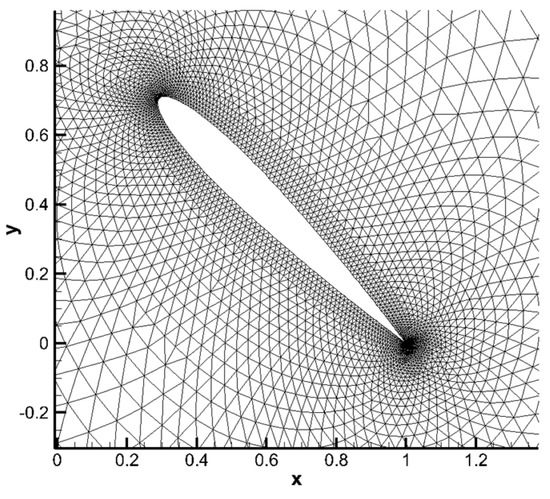
Figure 9.
Deformed mesh around the airfoil.
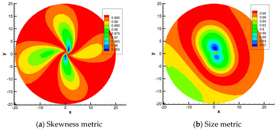
Figure 10.
Mapping-based metrics of test case 2.
In order to check the accuracy of mapping-based metrics of mesh deformation, a specific element with the minimal metrics value in the blue area is selected as Figure 11a shows with a red line. Same as described in Section 4.1, with the geometrical method, the angles of deformed mesh and the area ratio from initial mesh to deformed mesh can be calculated directly based on geometrical relationships. The geometric configuration of the specific element is presented in Figure 11b. is the angle between the sides joined at the th node in the element.
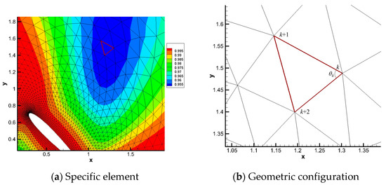
Figure 11.
Specific element with minimal skewness metrics.
Calculation results of an angle change have been presented in Table 5. It can be seen that calculation results by the mapping-based metric have a very small error compared to the geometrical calculation directly. The maximal error value is around 1%. The area ratio calculation results of mapping-based metrics is 0.824. It is very close to the result of the geometrical method, which has a value of 0.826 resulting in a small size ratio error around 0.24%. The very small errors of angle change and size ratio indicate that the mapping-based metrics method is suitable for evaluation of a mesh deforming algorithm for unstructured mesh.
Table 5.
Comparison between the mapping-based method and geometrical method.
Figure 12 and Figure 13 show the calculation results of traditional mesh-based metric described in Section 3.2 and Section 3.3 in this test case. For this unstructured mesh, all the elements are triangles. The skewness metric is used to measure the distortion, which contains both element angles and length ratios [35]. The mesh-based metric distribution is different from that of mapping-based metrics. Every two sides of any initial element are not parallel to the base vectors of initial configuration on which the mapping-based metric of deformation is based. Therefore, the comparison between mapping-based metrics and mesh-based metrics is useless.
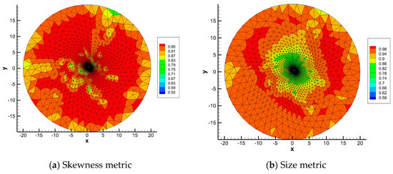
Figure 12.
Mesh-based metrics of test case 2.
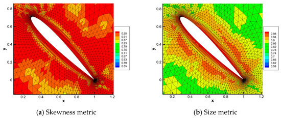
Figure 13.
Mesh-based metrics near the airfoil.
4.3. Test Case 3: Transform of Airfoil with a Viscous Layer
The mesh deformation algorithm performed very well for rigid airfoil with large rotation, as shown in Section 4.2. However, it is not clear how it works when the airfoil is changed. In this test case, an airfoil transform problem with a C-Type structure mesh are investigated. The initial airfoil is NACA0012, which is symmetrical and the target airfoil is NACA4412, which is asymmetric, as shown in Figure 14. Additionally, 100 nodes on the airfoil and 84 nodes on the boundary are selected as the center node. Figure 15 gives the deformed mesh over the calculation domain. Due to the small displacement of the nodes, it is almost impossible to detect the distortion of elements at a certain distance from the airfoil. Deformed mesh near the training edge and the leading edge of the airfoil has been given in Figure 15. As can be seen, the mesh near the airfoil maintains good orthogonality.
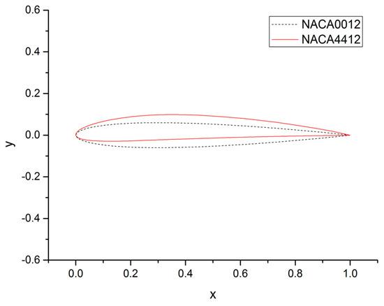
Figure 14.
Airfoil change in test case 3.
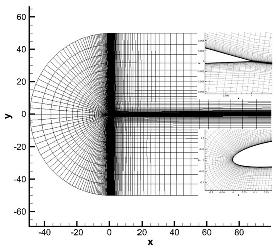
Figure 15.
Deformed mesh in test case 3.
Mapping-based metrics are used to illustrate the ability of the deformation. Figure 16 shows the calculation results of mapping-based metrics. The minimum value of skewness metrics of deformation is from the area around the leading edges, which is larger than 0.955. The area around the training edge experiences a relative heavy area change. However, the size metrics value is large than 0.85.
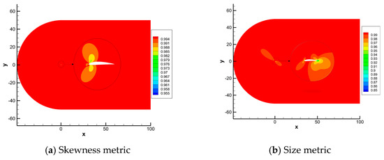
Figure 16.
Mapping-based metrics in test case 3.
For this case, the mesh far away from the airfoil is slightly deformed, and the quality of elements in a viscous layer should be paid more attention, especially the grid orthogonality. Figure 17 shows the skewness metrics and size metrics of each deformed mesh near the airfoil. The minimal value of skewness metrics is larger than 0.91 and size metrics is larger than 0.86. The deformed elements maintain good orthogonality and the area are also well preserved. Table 6 shows the comparison between two metrics and average metrics value has also been presented. All the average and minimal quality metrics of size and skew calculated by mapping-based metrics and traditional mesh-based metrics methods are closed, resulting in small error values of less than 0.35%.
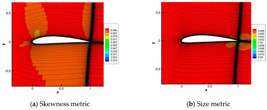
Figure 17.
Mesh quality near the airfoil.
Table 6.
Comparison between mapping-based metric and mesh-based metrics.
5. Conclusions
In this paper, the mapping-based metrics are established to evaluate the CFD mesh quality with a deforming algorithm. With no grid-connectivity information required, implementation of this method is relatively simple and efficient compared to traditional mesh-based metrics. RBFs’ method based on generalized TPS is tested with three test cases including structured and unstructured mesh. This method can handle large deformations of a mesh caused by translation, rotation, and airfoil transform, and it generates meshes with high quality after deformation. Mapping-based metrics are used to analyze the characteristics of this algorithm. A new point for mesh quality evaluation based on continuum mechanics is proposed.
Compared with a geometrical method, mapping-based metrics show high accuracy for an angle change and area change of a specific element. Meanwhile, when it is used to give the quality of deformed mesh, mapping-based metrics do not need the information of deform mesh. The method proposed here is efficient to calculate the quality of the mesh deformation process, especially for the dynamic cases to check if there are degradable problems. Meanwhile, the method has a high potential to be used in commercial software, which only needs the initial mesh coordinates and deformation vectors with uncomplicated calculations. The display of the results is consistent with existing software processing. Although the method in this paper is deduced by generalized TPS, the approach is consequently suitable for any other RBFs.
Finally, it should be noted that, because three 2-dimensional test cases are used, the calculation time and computing resource consumption is not different enough between a mesh-based metrics method and a new method proposed. In the next research, the mapping-based metrics method will be extended to a more complex problem in a 3-dimensional space, and the improvement of efficiency is expected.
Author Contributions
Conceptualization, S.J. and C.X. Methodology, C.X., C.A. and Y.L. Software, S.J. Validation, C.X., S.J. and C.A. Writing—original draft preparation, Y.L. and C.A. Writing—review and editing, S.J. and C.A. Visualization, C.X. and C.A. Project administration, C.Y. All authors have read and agreed to the published version of the manuscript.
Funding
This research was funded by the National Key Research and Development Program (2016YFB0200703).
Informed Consent Statement
Not applicable.
Data Availability Statement
The data presented in this study are available on request from the corresponding author. The data are not publicly available due to restriction of research funding.
Conflicts of Interest
The authors declare no conflict of interest.
References
- Jakobsson, S.; Amoignon, O. Mesh deformation using radial basis functions for gradient-based aerodynamic shape optimization. Comput. Fluids 2007, 36, 1119–1136. [Google Scholar] [CrossRef]
- Bano, T.; Hegner, F.; Heinrich, M.; Schwarze, R. Investigation of fluid-structure interaction induced bending for elastic flaps in a cross flow. Appl. Sci. 2020, 10, 6177. [Google Scholar] [CrossRef]
- An, C.; Yang, C.; Xie, C.C.; Yang, L. Flutter and Gust response analysis of a wing model including geometric nonlinearities based on a modified structural ROM. Chin. J. Aeronaut. 2020, 33, 48–63. [Google Scholar] [CrossRef]
- Borazjani, I.; Sotiropoulos, F. Numerical investigation of the hydrodynamics of anguilliform swimming in the transitional and inertial flow regimes. J. Exp. Biol. 2009, 212, 576–592. [Google Scholar] [CrossRef]
- Rinaudo, A.; Raffa, G.M.; Scardulla, F.; Pilato, M.; Scardulla, C.; Pasta, S. Biomechanical implications of excessive endograft protrusion into the aortic arch after thoracic endovascular repair. Comput. Biol. Med. 2015, 66, 235–241. [Google Scholar] [CrossRef] [PubMed]
- Zhao, R.; Li, C.; Guo, X.W.; Fan, S.J.; Wang, Y.; Yang, C.Q. A block iteration with parallelization method for the greedy selection in radial basis functions based mesh deformation. Appl. Sci. 2019, 9, 1141. [Google Scholar] [CrossRef]
- Cella, U.; Biancolini, M.E. Aeroelastic analysis of aircraft wind-tunnel model coupling structural and fluid dynamic codes. J. Aircr. 2012, 49, 407–414. [Google Scholar] [CrossRef]
- Pan, J.Y.; Liu, F. Wing flutter prediction by a small-disturbance Euler method on body-fitted curvilinear grids. AIAA J. 2019, 57, 4873–4884. [Google Scholar] [CrossRef]
- Li, C.; Xu, X.H.; Wang, J.W.; Xu, L.Y.; Ye, S.; Yang, X.J. A parallel multiselection greedy method for the radial basis function-based mesh deformation. Int. J. Numer. Methods Eng. 2018, 113, 1561–1588. [Google Scholar] [CrossRef]
- Banita, J.T. Unsteady Euler airfoil solutions using unstructured dynamic meshes. AIAA J. 1990, 28, 1381–1388. [Google Scholar]
- Banita, J.T. Unsteady Euler algorithm with unstructured dynamic mesh for complex-aircraft aerodynamic analysis. AIAA J. 1991, 29, 327–333. [Google Scholar]
- Fang, H.; Hu, Y.K.; Yu, C.H.; Tie, M.; Liu, J.; Gong, C.Y. An efficient radial basis functions mesh deformation with greedy algorithm based on recurrence choleskey decomposition and parallel computing. J. Comput. Phys. 2019, 377, 183–199. [Google Scholar]
- Pan, Y.; Yuan, Q.; Huang, G.G.; Gu, J.W.; Li, P.; Zhu, G.Y. Numerical investigations on the blade tip clearance excitation forces in an unshrouded turbine. Appl. Sci. 2020, 10, 1532. [Google Scholar] [CrossRef]
- Bottasso, C.L.; Detomi, D.; Serra, R. The ball-vortex method: A new simple spring analogy method for unstructured dynamic meshes. Finite Elem. Anal. Des. 2005, 41, 1118–1139. [Google Scholar]
- Farhat, C.; Degand, C.; Koobus, B. Torsional springs for two-dimensional dynamic unstructured fluid meshes. Comput. Methods Appl. Mech. Eng. 1998, 163, 231–245. [Google Scholar] [CrossRef]
- Blom, F.J. Considerations on the spring analogy. Int. J. Numer. Method Fluids 2000, 32, 647–668. [Google Scholar] [CrossRef]
- Zeng, D.H.; Either, C.R. A semi-torsional spring analogy model for updating unstructured meshes in 3D moving domain. Finite Elem. Anal. Des. 2005, 41, 1118–1139. [Google Scholar] [CrossRef]
- Witteveen, J. Explicit and robust inverse distance weighting mesh deformation for CFD. In Proceedings of the 48th AIAA Aerospace Science Meeting including the New Horizons Forum and Aerospace Exposition, Orlando, FL, USA, 4–7 January 2010. [Google Scholar]
- Gaitonde, A.L.; Fiddes, S.P.A. A moving mesh system for the calculation of unsteady flows. In Proceedings of the 31st Aerospace Science Meeting & Exhibit, Reno, NV, USA, 11–14 January 1993. [Google Scholar]
- Liu, X.; Qin, N.; Xia, H. Fast dynamic grid deformation based on Delaunay graph mapping. J. Comput. Phys. 2006, 211, 405–423. [Google Scholar] [CrossRef]
- Selim, M.M.; Koomullil, R.P.; Shehata, A.S. Incremental approach for radial basis functions mesh deformation using data reduction. J. Comput. Phys. 2016, 321, 997–1025. [Google Scholar]
- De Boer, A.; van der Schoot, M.S.; Bijl, H. Mesh deformation based on radial basis function interpolation. Comput. Struct. 2007, 85, 784–795. [Google Scholar] [CrossRef]
- Beckert, A.; Wendland, H. Multivariate interpolation for fluid-structure-interaction problems using radial basis functions. Aerosp. Sci. Technol. 2001, 5, 125–134. [Google Scholar] [CrossRef]
- Sheng, C.; Allen, C.B. Efficient mesh deformation using redial basis functions on unstructured meshes. AIAA J. 2012, 51, 707–720. [Google Scholar] [CrossRef]
- Bos, F.M.; van Oudheusden, B.W. Radial basis function based mesh deformation applied to simulation of flow around flapping wings. Comput. Fluids 2013, 79, 167–177. [Google Scholar] [CrossRef]
- Rendall, T.; Allen, C. Efficient mesh motion using radial basis functions with data reduction algorithm. J. Comput. Phys. 2009, 228, 6231–6249. [Google Scholar] [CrossRef]
- Wang, G.; Mian, H.H.; Ye, Z.Y.; Lee, J.D. Improved point selection method for hybrid-unstructured mesh deformation using radial basis function. AIAA J. 2015, 53, 1016–1025. [Google Scholar] [CrossRef]
- Michler, A.K. Aircraft control surface deflection using RBF-based mesh deformation. Int. J. Numer. Method Eng. 2011, 88, 986–1007. [Google Scholar] [CrossRef]
- Fang, H.; Gong, C.; Yu, C.; Min, C.; Zhang, X.; Liu, J.; Xiao, L. Efficient mesh deformation based on Cartesian background mesh. Comput. Math. Appl. 2017, 73, 71–86. [Google Scholar] [CrossRef]
- Xie, L.; Liu, H. Efficient mesh motion using radial basis functions with volume grid points reduction algorithm. J. Comput. Phys. 2017, 228, 6231–6249. [Google Scholar] [CrossRef]
- Knupp, P.M. Algebraic mesh quality metrics for unstructured initial meshes. Finite Elem. Anal. Des. 2003, 39, 217–241. [Google Scholar] [CrossRef]
- Goldberg, U. Pointwise turbulence modeling for engineering applications. In Proceedings of the International CFD Workshop on Supersonic Transport Design, Tokyo, Japan, 16–17 March 1998. [Google Scholar]
- Harder, R.L.; Desmarais, R.N. Interpolation using surface splines. J. Aircr. 1972, 9, 189–191. [Google Scholar] [CrossRef]
- Liu, I.S. Continuum Mechanics; Springer: Berlin/Heidelberg, Germany, 2002. [Google Scholar]
- Zou, S.; Yuan, X.F.; Yang, X.; Yi, W.; Xu, X. An integrated lattice boltzmann and finite volume method for the simulation of viscoelastic fluid flows. J. Non-Newton. Fluid Mech. 2014, 211, 99–113. [Google Scholar] [CrossRef]


Publisher’s Note: MDPI stays neutral with regard to jurisdictional claims in published maps and institutional affiliations. |
© 2020 by the authors. Licensee MDPI, Basel, Switzerland. This article is an open access article distributed under the terms and conditions of the Creative Commons Attribution (CC BY) license (http://creativecommons.org/licenses/by/4.0/).