Article

Prediction of Arrival Time of Vessels Considering Future Weather Conditions

1
Hitachi, Ltd., 292 Yoshidacho, Totsuka, Yokohama, Kanagawa 2440817, Japan
2
School of Knowledge Science, Japan Advanced Institute of Science and Technology (JAIST), 1-1 Asahidai, Nomi, Ishikawa 9231292, Japan
*
Author to whom correspondence should be addressed.
Appl. Sci. 2021, 11(10), 4410; https://doi.org/10.3390/app11104410
Submission received: 16 April 2021 / Revised: 4 May 2021 / Accepted: 11 May 2021 / Published: 13 May 2021
(This article belongs to the Section Applied Industrial Technologies)

Abstract

:
International logistics is becoming increasingly active. Marine transportation, in particular, accounts for approximately 90% of the total volume managed in international logistics and plays a vital role in the supply chains of many companies. However, en route factors, such as weather conditions, often delay scheduled arrivals at destination ports, and an accurate prediction of the arrival time is required for supply chain efficiency. The arrival time has been predicted in previous studies by calculating the route to the destination port and the en route voyage speed without considering the influence of future weather conditions. Hence, the prediction accuracy may decrease when weather conditions change. In this study, we propose a prediction method that identifies the route from the voyage results of vessels whose weather condition is similar to the future one and uses Bayesian learning to calculate the voyage speed in consideration of future weather conditions. Consequently, future changes in weather conditions are reflected in the prediction results. The prediction accuracy of the proposed method is projected to be 28% higher than that from previous studies based on historical operational data of vessels carrying home appliance and automobile industry cargoes.

1. Introduction

Free trade agreements (FTAs) and economic partnership agreements (EPAs) to eliminate tariffs between countries and regions continue to grow in number with progress in trade liberalization [1]. There has been an annual increase in the scale of cross-border electronic commerce (EC), which includes trading on online shopping sites across national borders. The EC market is projected to grow at an annual rate of 27% by 2027 [2]. The impact of these factors has made international logistics between countries and regions increasingly active. Figure 1 shows annual increases in the number of containers, in terms of twenty-foot equivalent units (TEU), handled in harbors around the world, where there was a 1.5-fold increase in the number of containers during the decade from 2008 to 2018 [3]. In particular, marine transportation accounts for approximately 90% of the total volume managed in international logistics and plays a vital role in the supply chains of many companies [4].
However, the impact of en route factors, such as weather conditions, may delay the scheduled arrival of a vessel at a destination port. Some consequences are delays in deliveries to customers and parts shortages at factories. A margin of error may be incorporated into the vessel transportation time to account for potential delays, and it can be used to develop procurement, production, and shipping plans at sites such as factories and sales companies. However, setting an excessive margin of error for the vessel transportation time results in surplus inventory [5]. An alternative to setting a uniform transportation time for vessels in advance is to sequentially predict the arrival time from future weather conditions. These prediction results are then used as a basis for operations, such as parts procurement, finished product assembly, and product shipment. This strategy can effectively reduce delivery delays and surplus inventory.
Considering the issues presented above, the objective of this study is the prediction of the arrival time of vessels to improve the efficiency of the supply chain associated with marine transportation. We refer the reader to a representative study by Alessandrini et al. on predicting the arrival times of vessels at a destination port [6]. Alessandrini et al. calculated the arrival time by predicting future routes from historical operation data for the vessel. However, the impact of future weather conditions on the sea route and voyage speed was not considered, which could lower the prediction accuracy for environments with changing weather conditions. In this study, a method is proposed to predict the arrival times of vessels in consideration of future weather conditions.
The remainder of this paper is structured as follows. An overview of previous studies on predicting the arrival times of vessels and corresponding challenges is presented in Section 2. The proposed prediction method is described in Section 3. The prediction accuracy of the proposed method is compared with that of a previous study based on the historical operation data of vessels carrying cargoes for the home appliance and automobile industries in Section 4. The results of the study are summarized in Section 5.

2. Previous Studies

An overview of previous studies on the prediction of arrival times of vessels and corresponding challenges is presented in this section.

2.1. Overview

To prevent collisions among vessels and save lives, the installation of an automatic identification system (AIS) for vessels has been mandatory since 2002 for passenger ships, vessels of 500 gross tonnage (GRT) or more, and vessels of 300 GRT or more that are engaged in international logistics [7]. The AIS relays dynamic information for a vessel, such as position information and the bow direction, as well as static information, such as the ship identification number, total length, and total tonnage, in international very high frequency (VHF) to terrestrial facilities. The AIS also receives information about other vessels from terrestrial facilities.
The introduction of AIS has facilitated the acquisition of operation data of vessels and led to the emergence of data providers, such as Marine Traffic, who accumulate and publish operational data of vessels worldwide [8]. Consequently, the use of operational data is being actively researched for routing and scheduling operations [9].
Here, there are many research works about routing scheduling operations for other modes of transportation such as automobiles and aircrafts. For example, one study predicted the short-term airport arrival time flow [10], and another study predicted an aircraft flight course and arrival time [11]. However, unlike other modes of transportation, vessels have some freedom in selecting routes, which has resulted in numerous studies on vessel routing. In recent years, the Dijkstra algorithm [12], which is often used to find the shortest path in problems, and its derivative, the A* algorithm [13,14,15], have been used in studies to calculate routes considering weather conditions. The machine learning models of support vector regression (SVR) and differential evolution (DE) have also been combined for use in route prediction [16]. Moreover, there are several studies which predict route and arrival delay with neural networks [17,18]. The effect of weather conditions on a vessel’s future voyage speed has also been predicted [19] by using equations of motion to model vessel motion. The prediction model includes parameters related to waves/winds, such as the wave height, wave period, and wind power, as well as parameters pertaining to dynamic vehicle information, such as the number of engine and propeller rotations, as well as the bow direction. The voyage speed is calculated using known parameters, such as the en route weather conditions and the engine output. Motion equations also are used to predict ship performance [20].
A representative study by Alessandrini et al. [6] predicted the arrival time at a destination port. This method consists of two steps: (A) predicting the route from the current position to the destination port and (B) predicting the en route voyage speed to calculate the time of arrival at the destination port.

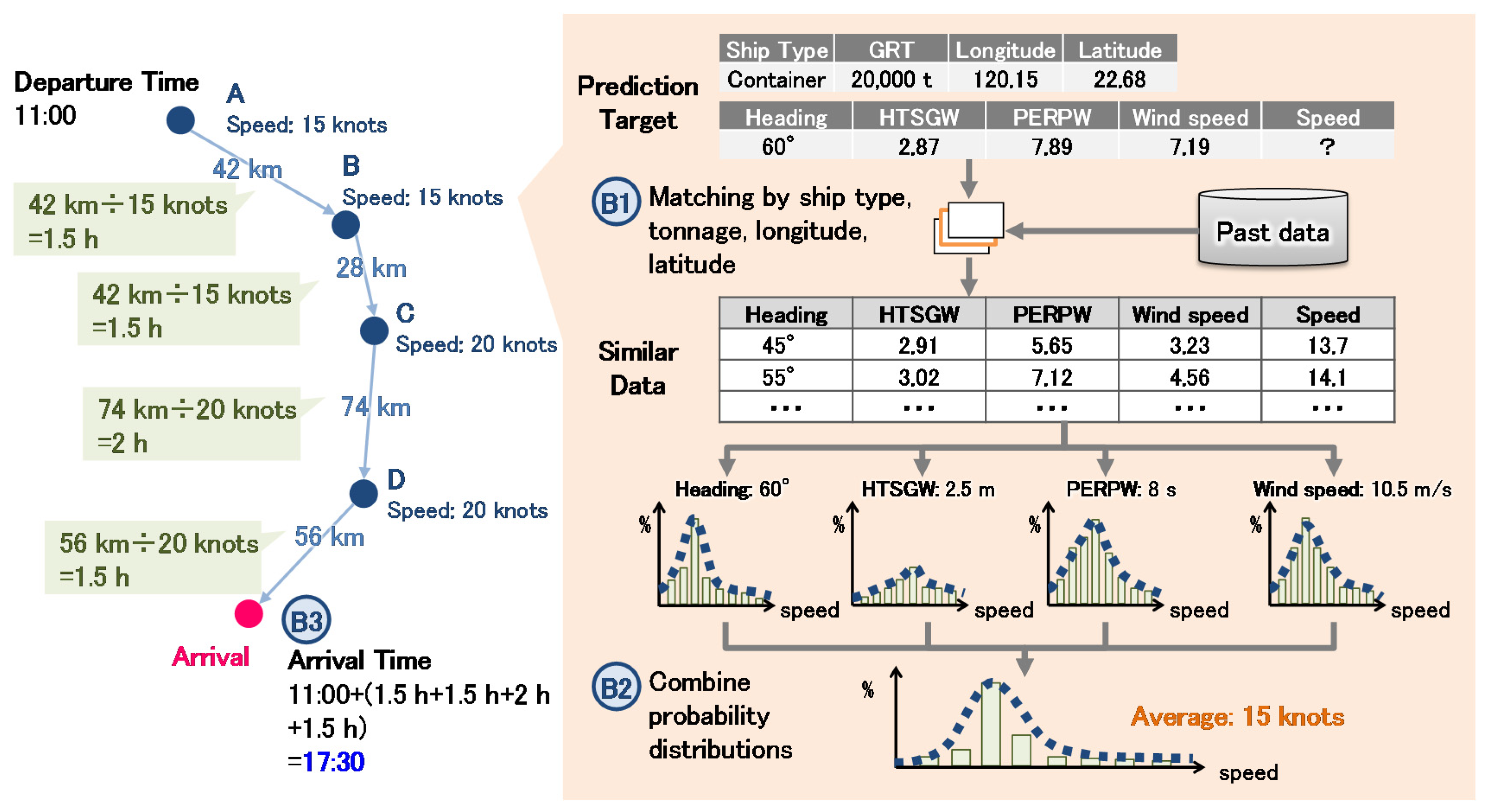
2.1.1. (A) Route Calculation

The Dijkstra method is used to determine the route that minimizes the travel distance from the current position to the destination port under the constraints of the topographical information and congestion status of vessels at each candidate transit site. The Dijkstra method is one of the algorithms available for determining the shortest route from a departure site to a destination site. The transit sites are represented at the vertex of the graph, the connection between the sites is represented at the edge, and the route is calculated in a way that minimizes the cost of traversing an edge. Alessandrini et al. set the cost of each edge in accordance with the distance traveled between sites, the congestion status at each candidate transit site, and the topographical information of each site regarding its location on land or sea.

2.1.2. (B) Voyage Speed Calculation

The en route voyage speed is calculated from past voyages with the same departure and destination ports, and it is used to calculate the time required to reach the destination port. First, data for the same departure and destination port are extracted from the operation data of the considered vessel, and the average voyage speed is calculated. The route obtained from (A) is used to calculate the distance from the current position to the destination port, which is then divided by the average voyage speed to yield the time required to reach the destination port. This time is added to the current time to determine the arrival time at the destination port.

2.2. Issues with Previous Studies

As presented in Section 2.1, Alessandrini et al. (A) calculated the route from the current position to the destination port and then (B) predicted the voyage speed and calculated the time required to reach the destination port. However, there are shortcomings with both (A) and (B), as discussed below.

2.2.1. (A) Issues with Route Calculations

Alessandrini et al. determined the route by minimizing the travel distance from the current position to the destination port under the constraints of the topographical information and congestion status of vessels at each candidate transit site. However, the future weather conditions are not considered in determining the route.
Generally, the captain decides the route on the basis of future weather conditions to ensure the safety of the vessel. Fujii et al. [21] used operational data to analyze the winter Pacific route from Japan to the United States. The eastbound voyage from Japan to the United States generally passes through the center of the Pacific Ocean to take advantage of tailwinds and the following sea from low-pressure systems. On the other hand, because the wind/head sea in the westbound voyage from the United States to Japan is opposite to that of the eastbound voyage, a vessel will take a northerly route through the vicinity of the Aleutian Islands or a southerly one instead of going through the center of the Pacific Ocean. As the method proposed by Alessandrini et al. does not consider the influence of these weather conditions, the same route is calculated for both east- and westbound voyages. Such deviations from the actual route can reduce the prediction accuracy of the arrival time.
Other studies mentioned in Section 2.1 also are not enough to predict the arrival time accurately. The study by Zhao et al. [10] predicted the flight arrival flow at an airport. However, it did not estimate the route and arrival time for each aircraft. The study by Kaushik et al. [11] predicted each aircraft’s route to a destination airport. However, it focused on short-distance routes with a linear system model; therefore, long-distance routes from departure to destination may not be estimated accurately. Although future weather conditions have been considered in other routing studies [14,15], they used the Dijkstra method or the A* algorithm to determine the shortest route to the destination port. However, as Fujii et al. have shown, the shortest route is not always taken in practice because of safety considerations. Therefore, these methods may produce deviations from the actual route to routes that are significantly affected by weather. Note as well that the studies by Liu et al. [16], Dimitrios et al. [17], and Dimitrios et al. [18] based on SVR and neural networks did not consider future weather conditions. Moreover, the study by Ruihua et al. [20] used the equations of vessel motion to calculate the ship performance and voyage route. However, the equations involve some parameters such as the viscous resistance that must be tuned in water tank experiments for each vessel model. As water tank experiments are not always representative of actual marine environments, it is difficult to determine parameters suitable for them.

2.2.2. (B) Issues with Voyage Speed Calculations

As discussed in Section 2.1, Alessandrini et al. used data on the departure and destination ports from operation data on the same vessel to calculate the average voyage speed. However, future weather conditions were not considered despite their potential effect on the voyage speed. The voyage speed also varies with the transit area, such as harbor, offshore, and strait, examples of which are shown in Figure 2. This figure is a graph created using Marine Traffic operation data on the voyage speed distribution of vessels around the Kanmon Straits, Kyushu, Taiwan, and Hong Kong ports in November 2019. The vertical axis depicts the percentage of vessels that made the voyage at the speed depicted on the horizontal axis. Figure 2 shows vessels travel at a high speed offshore but at a low average speed of 10 knots or less near straits and harbors. Alessandrini et al. did not consider these regional aspects of the voyage speed.
Moreover, as mentioned above, the method of Szelangiewicz et al. [19] uses equations of motion considering weather conditions and wave/wind parameters to calculate the voyage speed. Parameters such as the number of engine and propeller rotations are also considered. The effect of these parameters is small near ports and large offshore, and therefore they reflect the regionality of the voyage speed. However, just like the study by Ruihua et al. [20], the equations of motion also involve other parameters such as the viscous resistance that are difficult to determine as suitable for actual marine environments. In addition, operation data provided by an AIS do not include dynamic vessel information, such as the number of engine and propeller rotations, and some ships may not provide such log data, making the acquisition of these data difficult.
In summary, the previous methods may not predict the voyage speed, and in turn the arrival time, so accurately for voyages with constantly changing weather conditions.

3. Proposed Method

A method for predicting the arrival time of vessels is proposed in this section. The shortcomings of the method proposed by Alessandrini et al. were identified in Section 2.2. That is, (A) the route calculation does not include the future weather conditions that are typically considered to ensure vessel safety, and (B) the voyage speed calculation does not consider regionality or future weather conditions. To increase the prediction accuracy of the arrival time, the weather conditions, vessel safety, and regional voyage speeds should be considered in (A) and (B).
As Hayashi et al. [22] noted, the vessel route for (A) can be freely selected, and captains almost always employ the same selection criteria. Hence, given the influence of weather, a limited number of routes can be selected. We can use this consideration to calculate routes with little deviation from the actual ones; that is, we can analyze the past routes of target vessels and choose those routes whose weather conditions are similar to the current conditions.
As discussed in Section 2.2, Alessandrini et al. used past data on the considered vessel on routes with the same departure and destination ports to calculate the average voyage speed (B). In contrast, we consider the weather conditions and regionality of the voyage speed when calculating the voyage speed for each transit site along a route and thereby the time of arrival at the destination port. The voyage speed at each site is calculated from positional information, namely, the latitude and longitude, the weather information at each point, and past data, similar to the dynamic information of the vessel.
Here, the parameters adopted by Szelangiewicz et al. [19] are used to determine the dynamic information about the vessel and weather information. The parameters for the weather information are the wave height, wave period, and wind speed, while the bow direction is used as the parameter for the dynamic vessel information. Figure 3 shows the main parameters used in this study and in the study of Szelangiewicz et al. Here, our method incorporates the regionality of the voyage speed by replacing the parameters considered by Szelangiewicz et al., such as the number of engine and propeller rotations, with positional information, namely, the latitude and longitude.
However, there is only a limited amount of data in which all parameter sets such as the ship type, total tonnage, longitude, latitude, wave height, wave period, wind speed, and bow direction match, and the prediction accuracy will deteriorate when only a small quantity of data can be used. On the other hand, a sufficient amount of past data can be obtained for the individual parameters. Here, we can use Bayesian learning [23] to make estimations from small quantities of data by combining probability distributions for each parameter. In particular, our method generates a probability distribution of voyage velocities from the past data for every parameter and then combines the distributions. This strategy resolves the problem of limited data availability.
The route calculation and voyage speed calculation are detailed below.

3.1. (A) Route Calculation

An illustrative overview of the route calculation is illustrated in Figure 4. Steps A1 to A3 are used to find a route appropriate for the future weather conditions from the past routes of vessels similar to the considered vessel.
In step A1, routes with the same departure and destination ports are extracted from the data for vessels similar to the considered vessel. Although the use of past data for the same vessel would maximize the prediction accuracy, a sufficient amount of data may not be available for that vessel on the routes. Therefore, data for similar vessels are used in addition to data for the same vessel to ensure a sufficient quantity of data can be extracted. Although it is a challenging problem to identify similar vessels, vessel dimensions (such as the total length or width) can be determined from the vessel type (such as tankers or container vessels), weight, and GRT, as illustrated in Figure 4 [24]. Hence, a route that takes into account the current weather conditions can be extracted from past data for similar vessel types and GRTs. In the illustration, no vessels are found with exactly the same GRT as the considered vessel, so the order of GRT (e.g., 10,000-ton class, 20,000-ton class, or 30,000-ton class) is considered. Figure 5 shows an example where the considered vessel is a container ship with a GRT of 21,643, and data on similar container ships in the 20,000-ton GRT class are selected. In addition, some routes include outliers due to vessel breakdown, accidents, etc. The AIS information includes voyage status, and it can be used to remove routes including abnormal voyage statuses.
Step A2 consists of acquiring past and future weather conditions for each past route found in A1 and quantifying the error involved. The sets, indexes, and constants used in the quantification process are detailed below. Moreover, Figure 6 shows a graphical image of the sets, indexes, and constants. In Figure 6, quantification is conducted for two routes.
[Sets]
R O U T E Set of routes extracted in A1
S I T E r Set of transit sites along route r
[Index]
r R O U T E Route
s S I T E r Transit site
[Constants]
H T S G W r s P a s t Past wave height at a transit site s along route r
H T S G W r s F u t u r e Future wave height at a transit site s along route r
D I R P W r s P a s t Past wave direction at a transit site s along route r
D I R P W r s F u t u r e Future wave direction at a transit site s along route r
P E R P W r s P a s t Past wave period at a transit site s along route r
P E R P W r s F u t u r e Future wave period at a transit site s along route r
U G R D r s P a s t Past east–west winds at a transit site s along route r
U G R D r s F u t u r e Future east–west winds at a transit site s along route r
V G R D r s P a s t Past north–south winds at a transit site s along route r
V G R D r s F u t u r e Future north–south winds at a transit site s along route r
Among the constants presented above, the past wave height, wave direction, wave period, east–west winds, and north–south winds are acquired at the transit time for each site. The future constants cannot be similarly acquired because the future transit time for each site has not been determined. Therefore, the future constants are acquired by approximating the future transit time at each site as the time required to travel between the transit sites in the past. For example, Figure 4 shows that it takes one hour to travel from the departure port to site A; therefore, the future wave height, wave direction, wave period, east–west winds, and north–south winds at site A are determined for one hour from the current time. In this study, the above constants were obtained from the Research Institute for Sustainable Humanosphere, Kyoto University, which publishes weather data from the Japan Meteorological Agency [25]. In particular, we used grid point values (GPV) as the wave forecast and the global spectral model (GSM) as the wind forecast.
After acquiring the aforementioned constants, the error in the weather conditions at each site is calculated from the square of the error between the past and future constants. Equation (1) shows that the errors of all the sites can be summed to yield the error in the weather conditions for the route of interest. This process is applied to all the routes extracted in A1.
s ( H T S G W r s P a s t H T S G W r s F u t u r e ) 2 + ( D I R P W r s P a s t D I R P W r s F u t u r e ) 2 + ( P E R P W r s P a s t P E R P W r s F u t u r e ) 2 + ( U G R D r s P a s t U G R D r s F u t u r e ) 2 + ( V G R D r s P a s t V G R D r s F u t u r e ) 2
In step A3, the voyage calculated in A2 with minimal error in the weather conditions is selected to be the one whose weather is closest to the future conditions. Here, the errors in the weather conditions for different voyages are compared, and the route with the minimum error is chosen.

3.2. (B) Voyage Speed Calculation

An overview of the voyage speed calculation is illustrated in Figure 7. The time required to travel between sites and the time of arrival at the destination port are determined by calculating the voyage speed for each transit site in steps B1 to B3 described below.
In B1, past data are found for similar vessels at each transit site, i.e., the longitude and latitude of the transit site of interest and past data for vessels with similar GRTs and types. Here, there are only a few data with the exact longitudes and latitudes of the transit sites of interest, so data within ±0.1° of the exact latitudes and longitudes are used. As an example, the data shown in Figure 6 are longitudes ranging from 120.05 to 120.25 and latitudes ranging from 22.58 to 22.78.
In B2, Bayesian learning is used to derive the probability distribution of the voyage speeds by considering the bow direction and future weather conditions at each site, and the average speed is calculated. The probability distribution is updated on the basis of Bayes’ theorem given in Equation (2).
Posterior   distribution     prior   distribution × likelihood   function
Here, the prior and posterior distributions are the probability distributions of the estimation target before and after learning, respectively, and the likelihood is the probability distribution of the learning data. The symbol ∝ denotes that the term on the right side is proportional to the terms on the left side.
In this study, the estimation target is the voyage speed; the prior distribution is the probability distribution of the voyage speed generated from the data in B1; the likelihood function is the probability distribution of past data with similar bow directions, wave heights, wave periods, and wind speeds as the considered vessel; and the posterior distribution is the probability distribution of the voyage speed reflecting the likelihood function in the prior distribution. Note that both the prior distribution and likelihood function are histograms created using real data. Figure 8 illustrates how Bayesian learning is used to calculate the voyage speed. Bayes’ theorem is applied to each class of the histogram for the voyage speed. In Figure 8, the probability of distribution in the 10 knots class is 40%, which is calculated from the data in B1. Likelihood is calculated from the data of the ship whose heading is 60 degrees, HTSGW is 2.5 m, PERPW is 8 s, and wind speed is 10.5 m per second. Finally, the probability of posterior distribution is calculated by multiplying the prior distribution and likelihood, as shown in Equation (2), which is 11%. The same procedure is used for the other voyage speed classes, and the prior and posterior distributions are obtained by normalizing the calculated histogram to 1.
As mentioned above, the likelihood function is calculated from data for vessels with similar bow directions, wave heights, wave periods, and wind speed parameters, but very little data with exactly matching parameters are available. Therefore, as shown below, the likelihood function is calculated by generating a probability distribution for each parameter and combining the probability distributions. The random variables used in this calculation are defined as follows.
v Voyage speed
H e a d i n g Bow direction
H T S G W Wave height
P E R P W Wave period
W i n d S p e e d Wind speed
In the following equations, p represents the probability distribution, and the prior distribution of the voyage speed is represented by p(v). Substituting these variables into Bayes’ theorem given by Equation (2) yields the following expression.
p ( v | H e a d i n g ,   H T S G W ,   P E R P W ,   W i n d P o w e r ) p ( H e a d i n g ,   H T S G W ,   P E R P W ,   W i n d P o w e r | v ) × p ( v )
p ( H e a d i n g ,   H T S G W ,   P E R P W ,   W i n d P o w e r | v ) is the likelihood function for the conditional probability of the voyage speed v . The definition of the conditional probability can be used to rewrite this expression using four terms.
p ( H e a d i n g ,   H T S G W ,   P E R P W ,   W i n d P o w e r | v ) = p ( H e a d i n g | v ) × p ( H T S G W | v ) * p ( P E R P W | v ) × p ( W i n d P o w e r | v )
p ( H e a d i n g | v ) is the conditional probability for the bow direction, p ( H T S G W | v ) is the conditional probability for the wave height, p ( P E R P W | v ) is the conditional probability for the wave period, and p ( W i n d P o w e r | v ) is the conditional probability for the wind speed. The number of data can be obtained by calculating the conditional probability for each of these parameters. Thus, the likelihood function can be calculated using Equation (4). By splitting up the probability distribution as shown in Equation (4), even when there is only a small amount of data, Bayesian learning can estimate more accurately than other methods such as support vector machine.
The conditional probability of each parameter is calculated as follows. Figure 7 shows an example where the bow direction of the prediction target vessel is 60°. The percentage of vessels found in B1 with a bow direction of 60° is calculated for each voyage speed, where an example of this process is shown in Figure 8 for a voyage speed of 10 knots. The same procedure is followed for the other parameters, and the likelihood function is calculated.
In B3, the time required for travel from the current location to the destination port is calculated using the distance between sites and the voyage speed at each transit site. The time of arrival at the destination port is subsequently calculated. In Figure 7, the voyage speed at site A is 15 knots, and the distance between sites A and B is 42 km. Therefore, the time required to travel from A to B is calculated as 42 km ÷ 15 knots = 1.5 h. This process is repeated for all sites, and the time required to reach the destination port is calculated as 1.5 + 1.5 + 2 + 1.5 = 6.5 h. Adding this required time to the departure time of 11:00 results in a calculated time of arrival at the destination port of 17:30. Note that the great-circle distance between two sites is used in this study.

4. Verification of the Prediction Accuracy of the Proposed Method

The accuracy of the prediction method in Section 3 is verified in this section. Among the previous methods described in 2.1, those of Shin et al. [14], Pennino et al. [15], and Liu et al. [16] calculate the optimal voyage route but do not predict the arrival time. Moreover, the study of Szelangiewicz et al. [19] only focused on calculating the future voyage speed. Consequently, in this study, the method of Alessandrini et al. [6] was chosen for comparison. We use historical operation data of vessels traveling between Japan and Taiwan with home appliance-related cargoes and between Japan and the United States with automobile industry-related cargoes. The target vessels and their routes are shown in Table 1.
In Table 1, TS TOKYO and TS OSAKA are vessels with home appliance cargoes and NEW CENTURY 1 and NEW CENTURY 2 are the vessels with automobile industry cargoes. Four routes are considered for TS TOKYO and TS OSAKA: between Kobe and Nagoya, Nagoya and Yokohama, Tokyo and Keelung (Taiwan), and Keelung and Taichung (Taiwan). One route is considered for NEW CENTURY 1 and NEW CENTURY 2 between Toyohashi and Long Beach (USA). The arrival time to the destination port is predicted for each route.
The past vessel data used to predict the arrival time for each respective vessel are given below. All the past data were acquired from Vessel Historical Track and Berth Calls, which are APIs provided by Marine Traffic.
  • TS TOKYO, TS OSAKA
A total of 405 routes between Japan and Thailand sailed by 13 vessels from January 2019 to March 2020 carrying home appliance industry cargoes
  • NEW CENTURY 1, NEW CENTURY 2
A total of nine routes between Toyohashi (Japan) and Long Beach (USA) sailed by eight vessels
Moreover, as described in Section 3.1, the past weather data were obtained from the Research Institute for Sustainable Humanosphere, Kyoto University. Table 2 shows a part of the past vessel data. As shown in Table 2, we link voyage data and weather data based on each datum’s longitude and latitude. Each column contains the following information. MMSI, SPEED, LON, LAT, COURSE, HEADING, and TIMESTAMP are from voyage data. Moreover, HTSGW, PERPW, DIRPW, UGRD, and VGRD are from weather data. These columns’ meanings are shown in Table 3.
In this verification, the mean absolute percentage error (MAPE) for each voyage is calculated as shown in Equation (5).
M A P E = | ( P r e d i c t e d   a r r i v a l   t i m e D e p a r t u r e   t i m e ) ( A c t u a l   a r r i v a l   t i m e D e p a r t u r e   t i m e ) A c t u a l   a r r i v a l   t i m e D e p a r t u r e   t i m e | × 100   ( % )
We evaluate prediction accuracy with Equation (6) which is the MAPE subtracted from 100% so that the prediction accuracy is higher as the predicted arrival time is closer to the actual arrival time.
P r e d i c t i o n   a c c u r a c y = 100   ( % ) M A P E
Table 4 shows the results for the ten routes listed in Table 1. The proposed method has a higher prediction accuracy than the method of Alessandrini et al. for all ten routes. The mean prediction accuracy is 90% for the proposed method and 62% for the method of Alessandrini et al. Thus, the proposed method is more accurate than the method of Alessandrini et al.
To verify the proposed method’s advantages, its prediction accuracy was verified on 30 other routes between Japan and Taiwan. The mean prediction accuracies of the proposed method and the method of Alessandrini et al. were calculated with Equation (6). As a result, the mean prediction accuracy of 30 routes is 85% for the proposed method compared with 69% for the method of Alessandrini et al. More detailed results are shown in Appendix A. Moreover, we evaluate whether there is statistical significance of the difference between their mean prediction accuracies with a t-test whose significance level is 0.05. As a result, the 95% confidence interval of the difference between their mean prediction accuracies is from 0.081 to 0.23, the degree of freedom is 29, and the t-value is 4.03. The p-value is 0.00036 which is smaller than the significance level of 0.05. Therefore, there is statistical significance between the mean prediction accuracies. Thus, it is confirmed that the proposed method can predict the arrival time more accurately.
Figure 9 shows the actual route taken by TS OSAKA, which departed from KEELUNG on 29 April 2020 at 11:30 a.m. and compares the arrival times and routes predicted using the method of Alessandrini et al. and the proposed method. The route obtained using the predicted method is closer to the actual route than the one obtained by Alessandrini et al. However, the arrival time predicted by the proposed method is three hours earlier than the actual arrival time, which may result from a detour the vessel took before entering Taichung port (see the pink circle in Figure 9). As the voyage speed during the detour was 5 knots or lower, Taichung port may have been crowded, delaying vessel entry into the port.
We have shown that the proposed method is more accurate than the one of Alessandrini et al. for predicting the time of arrival to the destination port. The congestion status en route or at the destination port can also affect the prediction accuracy. Therefore, the congestion status at the destination port will be considered in a future study to increase the prediction accuracy of the proposed method.

5. Conclusions

To improve supply chain efficiency, we developed a highly accurate method for predicting the arrival time of marine transportation vessels, which account for approximately 90% of the total volume managed in international logistics and consume considerable time resources. The impact of en route factors, such as weather conditions, often prevents marine transportation vessels from arriving at the destination port as scheduled. The arrival time has been predicted in previous studies by calculating the route to the destination port and the en route voyage speed without considering the influence of future weather conditions. Therefore, the prediction accuracy may become low when weather conditions change.
In this study, a prediction method for the vessel arrival time was developed to consider weather conditions in two steps: (1) route calculation and (2) voyage speed calculation. (1) Past routes of vessels with similar GRTs and types as the considered vessel are obtained, the difference between future and past weather conditions is calculated for each route, and the route with the smallest difference is selected. (2) For each site along the route calculated in (1), past operation data under similar future weather conditions are acquired for vessels of similar type and GRT to the considered vessel. Bayesian learning is then used to calculate the voyage speed by considering the bow direction and future weather conditions at each site. The time required to travel to each site is then calculated by dividing the distance between sites by the voyage speed at each site and used to predict the time of arrival at the destination port.
The prediction accuracy of the proposed method was verified for vessels carrying cargoes for the home appliance and automobile industries. The mean prediction accuracy for ten vessels was 90% using the proposed method and 62% using the method of Alessandrini et al. [6]. Hence, the prediction accuracy for the arrival time is projected to increase by 28% compared with that of Alessandrini et al.
The congestion status en route and at the destination port will be considered in a future study to improve the prediction accuracy of the proposed method.

Author Contributions

Conceptualization, T.O. and T.I.; methodology, T.O. and T.I.; software, T.I.; validation, T.O. and T.I.; formal analysis, T.O. and T.I.; investigation, T.O. and T.I.; resources, T.O. and T.I.; data curation, T.I.; writing—original draft preparation, T.I.; writing—review and editing, T.O.; visualization, T.O., T.I. and N.U.; supervision, T.O.; project administration, T.O.; funding acquisition, T.O. All authors have read and agreed to the published version of the manuscript.

Funding

No external funding was obtained to conduct this study.

Institutional Review Board Statement

Not applicable.

Informed Consent Statement

Not applicable.

Data Availability Statement

Data is contained within the article.

Conflicts of Interest

The authors declare no conflict of interest.

Appendix A

Table A1 shows prediction results for the 30 import/export routes between Japan and Taiwan mentioned in Section 4.
Table A1. Routes.
Table A1. Routes.
Vessel NameTarget VoyageDeparture TimeArrival TimePrediction Accuracy
DepartureArrivalActualProposed MethodPrevious ResearchProposed MethodPrevious Research
TS TOKYONAGOYAYOKOHAMA2020/3/22 6:142020/3/22 22:302020/3/22 21:082020/3/23 3:0892%71%
TS TOKYONANSHAOSAKA2020/3/16 4:582020/3/19 23:142020/3/20 3:492020/3/20 6:1295%92%
TS TOKYOKOBENAGOYA2020/3/21 2:482020/3/21 22:192020/3/21 19:432020/3/22 2:4087%78%
TS TOKYOTOKYOKEELUNG2020/3/24 6:112020/3/27 5:402020/3/27 11:462020/3/27 18:0391%83%
TS TOKYOKEELUNGTAICHUNG2020/3/27 11:522020/3/27 19:432020/3/27 20:122020/3/27 18:3294%85%
TS TOKYOTAICHUNGKAOHSIUNG2020/3/28 3:522020/3/28 12:262020/3/28 15:132020/3/28 18:1067%33%
TS TOKYOKAOHSIUNGNANSHA2020/3/28 18:382020/3/30 0:082020/3/30 5:412020/3/30 3:0181%90%
TS TOKYOLAEM CHABANGHONG KONG2020/4/9 5:322020/4/13 4:332020/4/13 5:272020/4/12 22:3199%94%
TS TOKYONANSHAOSAKA2020/4/14 10:242020/4/17 23:062020/4/18 7:442020/4/18 11:5090%85%
TS TOKYOKEELUNGTAICHUNG2020/5/20 9:442020/5/20 17:052020/5/20 16:482020/5/20 16:2496%91%
TS TOKYOTAICHUNGKAOHSIUNG2020/5/20 22:462020/5/21 7:162020/5/21 9:362020/5/21 13:0472%32%
TS TOKYOKAOHSIUNGNANSHA2020/5/21 15:352020/5/23 1:542020/5/22 22:262020/5/22 23:5890%94%
APL PUSANNAGOYAKOBE2020/4/1 15:272020/4/2 22:112020/4/2 8:382020/4/2 9:5756%60%
APL PUSANNAGOYAKOBE2020/4/29 6:272020/4/30 22:042020/4/29 23:192020/4/30 0:5743%47%
HORAI BRIDGEHONGKONGKAOHSIUNG2020/4/6 21:482020/4/7 21:082020/4/7 22:012020/4/8 12:5596%32%
APL JEDDAHKAOHSIUNGYOKOHAMA2020/5/1 6:302020/5/4 21:392020/5/4 17:472020/5/5 9:2996%86%
APL JEDDAHTOKYONAGOYA2020/5/5 20:102020/5/6 10:232020/5/6 13:572020/5/6 19:3575%35%
APL JEDDAHNAGOYAKOBE2020/5/6 20:182020/5/7 21:512020/5/7 13:262020/5/7 14:4867%72%
WHITE DRAGONHONGKONGKAOHSIUNG2020/5/11 9:492020/5/12 11:552020/5/12 10:022020/5/13 0:5693%50%
TS OSAKAKOBENAGOYA2020/5/21 6:172020/5/22 4:292020/5/21 23:062020/5/22 6:0976%92%
TS OSAKANAGOYAYOKOHAMA2020/5/22 13:332020/5/23 1:442020/5/23 5:072020/5/23 10:2772%28%
TS OSAKATOKYOKEELUNG2020/5/23 20:152020/5/26 23:132020/5/26 19:532020/5/27 8:0796%88%
TS OSAKATAICHUNGKAOHSIUNG2020/5/28 2:492020/5/28 11:472020/5/28 13:392020/5/28 17:0779%40%
TS OSAKAKAOHSIUNGNANSHA2020/5/28 21:412020/5/30 4:362020/5/30 5:402020/5/30 6:0497%95%
TS KAOHSIUNGKOBENAGOYA2020/6/5 5:202020/6/5 22:092020/6/5 22:142020/6/6 5:1299%58%
TS KAOHSIUNGNAGOYAYOKOHAMA2020/6/6 7:112020/6/6 22:032020/6/6 22:422020/6/7 4:0596%59%
TS KAOHSIUNGTOKYOKEELUNG2020/6/8 3:402020/6/11 4:232020/6/11 3:142020/6/11 15:3298%85%
TS KAOHSIUNGKEELUNGTAICHUNG2020/6/11 11:132020/6/11 18:212020/6/11 19:112020/6/11 17:5388%94%
TS KAOHSIUNGTAICHUNGKAOHSIUNG2020/6/12 0:302020/6/12 9:052020/6/12 10:252020/6/12 14:4884%33%
TS KAOHSIUNGKAOHSIUNGNANSHA2020/6/12 19:112020/6/14 9:052020/6/14 0:132020/6/14 3:3477%85%

References

  1. Regional Trade Agreements DataBase. Available online: http://rtais.wto.org/UI/PublicMaintainRTAHome.aspx (accessed on 12 January 2021).
  2. Cross-Border B2C E-Commerce Market. Available online: https://www.zionmarketresearch.com/report/cross-border-b2c-e-commerce-market (accessed on 12 January 2021).
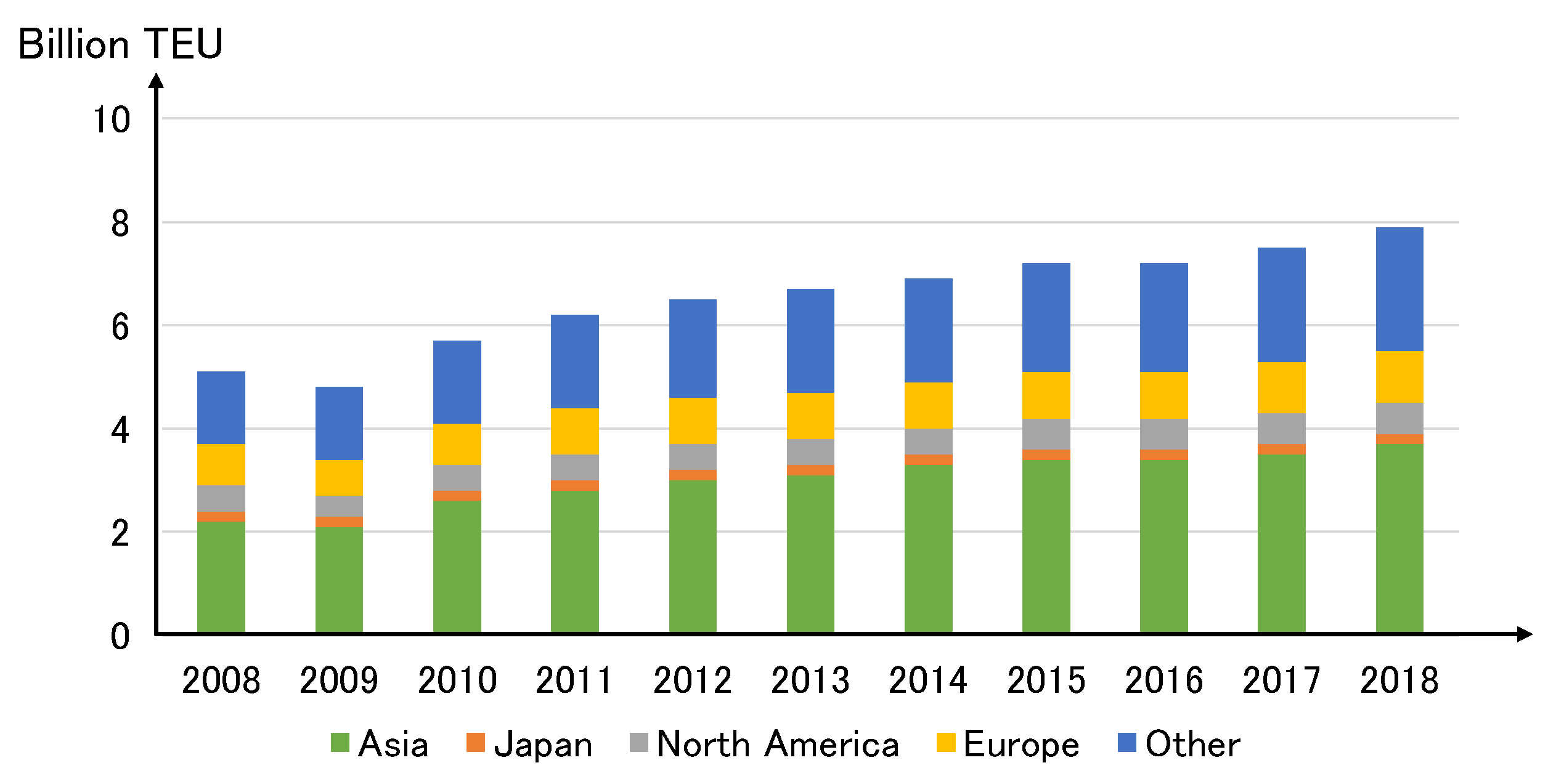
  3. Container Port Traffic (TEU: 20 Foot Equivalent Units). Available online: https://data.worldbank.org/indicator/IS.SHP.GOOD.TU (accessed on 12 January 2021).
  4. Pallotta, G.; Vespe, M.; Bryan, L. Vessel pattern knowledge discovery from AIS data: A framework for anomaly detection and route prediction. Entropy 2013, 15, 2218–2245. [Google Scholar] [CrossRef] [Green Version]
  5. Zhao, J.; Ji, M.; Feng, B. Smarter supply chain: A literature review and practices. J. DataInf. Manag. 2020, 2, 95–110. [Google Scholar] [CrossRef] [Green Version]
  6. Alessandrini, A.; Mazzarella, F.; Vespe, M. Estimated time of arrival using historical vessel tracking data. IEEE Trans. Intell. Transp. Syst. 2019, 20, 7–15. [Google Scholar] [CrossRef]
  7. Technical Characteristics for an Automatic Identification System Using Time Division Multiple Access in the VHF Maritime Mobile Frequency. Available online: http://www.itu.int/dms_pubrec/itu-r/rec/m/R-REC-M.1371-5-201402-I!!PDF-E.pdf (accessed on 12 January 2021).
  8. Marine Traffic. Available online: https://www.marinetraffic.com (accessed on 12 January 2021).
  9. Christiansen, M.; Fagerholt, K.; Nygreen, B.; Ronen, D. Ship routing and scheduling in the new millennium. Eur. J. Oper. Res. 2013, 228, 467–483. [Google Scholar] [CrossRef]
  10. Yang, Z.; Wang, Y.; Li, J.; Liu, L.; Ma, J.; Zhong, Y. Airport arrival flow prediction considering meteorological factors based on deep-learning methods. Hindawi Complex. 2020. [Google Scholar] [CrossRef]
  11. Roy, K.; Levy, B.; Tomlin, C. Target tracking and estimated time of arrival (ETA) prediction for arrival aircraft. In Proceedings of the AIAA Guidance, Navigation, and Control Conference and Exhibit, Colorado, CO, USA, 21–24 August 2006; pp. 1–22. [Google Scholar]
  12. Dijkstra, E.W. A note on two problems in connection with graphs. Numer. Math. 1959, 1, 269–271. [Google Scholar] [CrossRef] [Green Version]
  13. Hart, P.E.; Nilsson, N.J.; Raphael, B. A formal basis for the heuristic determination of minimum cost paths. IEEE Trans. Syst. Sci. Cybern. 1968, 4, 100–107. [Google Scholar] [CrossRef]
  14. Shin, Y.W.; Abebe, M.; Noh, Y.; Lee, S.; Lee, I.; Kim, D.; Bae, J.; Kim, K.C. Near-optimal weather routing by using improved A* algorithm. Appl. Sci. 2020, 10, 6010. [Google Scholar] [CrossRef]
  15. Pennino, S.; Gaglione, S.; Innac, A.; Piscopo, V.; Scamardella, A. Development of a new ship adaptive weather routing model based on seakeeping analysis and optimization. J. Mar. Sci. Eng. 2020, 8, 270. [Google Scholar] [CrossRef]
  16. Liu, J.; Shi, G.; Zhu, K. Vessel trajectory prediction model based on ais sensor data and adaptive chaos diffrential evolution support vector regression (ACDE-SVR). Appl. Sci. 2019, 9, 2983. [Google Scholar] [CrossRef] [Green Version]
  17. Dimitrios, Z.; Elias, X.; Dimitrios, L. Real-time vessel behavior prediction. Evol. Syst. 2016, 7, 29–40. [Google Scholar]
  18. Yu, J.; Tang, G.; Song, X.; Yu, X.; Qi, Y.; Li, D.; Zhang, Y. Ship arrival prediction and its value on daily container terminal operation. Ocean Eng. 2018, 157, 73–86. [Google Scholar] [CrossRef]
  19. Szelangiewicz, T.; Żelazny, K. Mathmatical model for predicting the ship speed in the actual weather conditions on the planed ocean route. New Trends Prod. Eng. 2018, 1, 5–112. [Google Scholar]
  20. Lu, R.; Turan, O.; Boulougouris, E. Voyage optimisation: Prediction of ship specific fuel consumption for energy efficient shipping. In Proceedings of the Low Carbon Shipping Conference, London, UK, 9–10 September 2013; pp. 1–11. [Google Scholar]
  21. Fujii, M.; Hashimoto, H.; Taniguchi, Y. Analysis of satellite AIS data to derive weather judging criteria for voyage route selection. Int. J. Mar. Navig. Saf. Sea Transp. 2017, 11, 271–277. [Google Scholar] [CrossRef] [Green Version]
  22. Hayashi, M.; Ishida, H. Characteristic analysis of weather routing by practical navigators. In Proceedings of the IEEE International Conference of Systems, Man and Cybernetics, Taiwan, China, 8–11 October 2006; pp. 786–790. [Google Scholar]
  23. Bishop, C. Pattern Recognition and Machine Learning; Springer: New York, NY, USA, 2006; ISBN 978-0-387-31073-2. [Google Scholar]
  24. Technical Note of National Institute for Land and Infrastructure Management. Available online: http://www.ysk.nilim.go.jp/kenkyuseika/pdf/ks0991.pdf (accessed on 14 January 2021).
  25. Research Institute for Sustanable Humanosphere, Kyoto University. Available online: http://database.rish.kyoto-u.ac.jp/arch/jmadata/gpv-original.html (accessed on 12 January 2021).
Figure 1. Growth in number of containers over last 10 years from 2008 to 2018 [3].
Applsci 11 04410 g001
Figure 2. Voyage speed distribution for various areas.
Applsci 11 04410 g002
Figure 3. Comparison between this study and a previous study.
Applsci 11 04410 g003
Figure 4. Overview of vessel routing procedure.
Applsci 11 04410 g004
Figure 5. Example of similar vessels.
Applsci 11 04410 g005
Figure 6. Graphical image of quantification.
Applsci 11 04410 g006
Figure 7. Overview of the procedure used to calculate the voyage speed.
Applsci 11 04410 g007
Figure 8. Using Bayesian learning to estimate the voyage speed distribution.
Applsci 11 04410 g008
Figure 9. Comparison of ship routes from KEELUNG to TAICHUNG.
Applsci 11 04410 g009
Table 1. Target vessels used to verify the prediction method.
Vessel NameDeparture PortArrival PortDeparture Time
TS TOKYOKOBENAGOYA2020/4/18 16:44
NAGOYAYOKOHAMA2020/4/19 17:48
TOKYOKEELUNG2020/4/22 10:24
KEELUNGTAICHUNG2020/4/25 18:32
TS OSAKAKOBENAGOYA2020/4/23 11:18
NAGOYAYOKOHAMA2020/4/24 12:08
TOKYOKEELUNG2020/4/26 2:23
KEELUNGTAICHUNG2020/4/29 11:30
NEW CENTURY 1TOYOHASHILONG BEACH2020/8/8 10:18
NEW CENTURY 22020/7/30 10:08
Table 2. Example of past vessel data.
MmsiSpeedLonLatCourseHeadingTimestampHtsgwPerpwDirpwUgrdVgrd
538007662164136.93834.616433153152019/1/1 0:011.055.103204.81−4.45
538007662173136.769734.8554303592019/1/1 1:0000−101.52−1.91
5380076620136.741334.9763393392019/1/1 1:5900−102.01−0.381
Table 3. Meaning of Table 2 columns.
Column NameMeaning
MMSIMaritime Mobile Service Identity
SPEEDVoyage speed of transit site
LONLongitude of transit site
LATLatitude of transit site
COURSEVoyage direction at transit site
HEADINGVessel direction at transit site
TIMESTAMPPassing time as transit site
HTSGWSignificant wave height
PERPWPrimary wave mean period
DIRPWPrimary wave direction
UGRDNorth–south wind component
VGRDEast–west wind component
Table 4. Comparison of prediction accuracy.
Vessel NameTarget VoyageArrival TimePrediction Accuracy
DepartureArrivalActualProposed MethodPrevious ResearchProposed MethodPrevious Research
TS TOKYOKOBENAGOYA2020/4/19 8:572020/4/19 10:562020/4/19 16:3588%
(2 h)
53%
(7.7 h)
NAGOYAYOKOHAMA2020/4/20 8:382020/4/20 8:162020/4/20 14:4298%
(–0.4 h)
59%
(6.1 h)
TOKYOKEELUNG2020/4/25 10:282020/4/25 14:192020/4/25 21:5595%
(3.9 h)
84%
(11.5 h)
KEELUNGTAICHUNG2020/4/26 2:032020/4/26 2:062020/4/26 1:1299%
(0.1 h)
89%
(–0.8 h)
TS OSAKAKOBENAGOYA2020/4/24 2:412020/4/24 5:302020/4/24 11:1082%
(2.8 h)
45%
(8.5 h)
NAGOYAYOKOHAMA2020/4/25 1:132020/4/25 3:592020/4/25 9:0279%
(2.8 h)
40%
(7.8 h)
TOKYOKEELUNG2020/4/28 23:282020/4/29 4:022020/4/29 13:5493%
(4.6 h)
79%
(14.4 h)
KEELUNGTAICHUNG2020/4/29 22:572020/4/29 19:382020/4/29 18:1071%
(–3.3 h)
58%
(–4.8 h)
NEW CENTURY 1TOYOHASHILONG BEACH2020/8/21 6:122020/8/21 7:542020/8/26 13:5599%
(2.3 h)
59%
(127.7 h)
NEW CENTURY 22020/8/12 6:042020/8/12 8:222020/8/17 13:4599%
(1.7 h)
50%
(127.7 h)
Publisher’s Note: MDPI stays neutral with regard to jurisdictional claims in published maps and institutional affiliations.

