2.1. Fish Image Dataset
Four fish species that are popular in the Mediterranean diet were studied:
Dicentrarchus labrax (sea bass),
Diplodus puntazzo,
Merluccius merluccius (cod fish) and
Sparus aurata (sea bream). Except for the cod fish, the rest of the species are also cultured in fish farms. ImageNet [
25] and other popular databases contain only a small number of fish images. For example, ImageNet contains
whales,
devilfish,
anemonefish,
lionfish,
blowfish and
garfish, but none of these species are studied in this paper. There are several other fish image datasets that can be found in [
26], but (1) there are not many photographs available for the specific species and (2) they are mainly photographs taken from ashore.
In this work, we focus on profile fish photographs taken from the side of the fish. Alternative ways to reassure that a fish is captured when its side is parallel with the camera image plane are the following: (1) trap the fish in a fishway where it will not have many degrees of freedom for a while, (2) examine a number of consecutive video frames and select the one where the fish has its maximum dimensions and (3) apply affine coordinate transformations to rotate appropriately a slanted fish contour before measuring its dimensions [
7]. In the affine transformation between two planes, a point
p(1) in the first plane with coordinates
was mapped to
in the second plane. A rotation matrix
multiplied the coordinates of
p(1), and an offset was potentially added to get
p(2). The
ra,
rb and offset values that maximized the fish contour dimensions could be selected, since a slanted or rotated fish seemed to have smaller dimensions than a fish in the expected position.
Since we generally did not know the distance of the fish, only relative distances and areas could be estimated. However, if the fish was captured when it passed a narrow fishway [
5], or if two photographs were taken from different cameras, the absolute dimensions and fish mass could also be estimated, as will be explained in
Section 2.4. The contribution of light refraction was negligible, but correction methods could also be applied to improve the accuracy. From the four fish families that were examined, the cod fish and sea bass had long bodies with small heights, while the sea bream and
Diplodus puntazzo had shorter lengths and bigger heights. The dataset used consisted of 25 photographs from each species. Many of these photographs were captured underwater. In the deep learning approach, the dataset was augmented using mirror images, jitter and random crop. In this way, a final training dataset that consisted of 4000 images was produced. Three quarters of them displayed fish, and the rest of them displayed a small part of the fish or background. Similar to [
20], the background could be as simple as seawater only, or it could contain more complex structures and objects. The size of the original images was 80 × 160, and this size was used in the image processing approach. The photographs were resized to 224 × 224 pixels in the deep learning approach to comply with the pretrained model that would be used, as will be explained in the following paragraphs.
The photographs that populated our dataset were retrieved from [
26], and others were publically available on the Internet. An initial dataset of 25 photograms per species is not adequately large for deep learning techniques. However, it is interesting to measure the accuracy that can be achieved in this case, since future versions of our system may also have to be trained with a small number of photographs to support a new species. In the image processing approach, three representative shape patterns were used for each species in order to apply pattern matching. In the deep learning approach, 15 of the 25 photographs from each species were used for training, and all the photographs were used for testing (due to the small dataset size).
2.2. Image Processing Approach
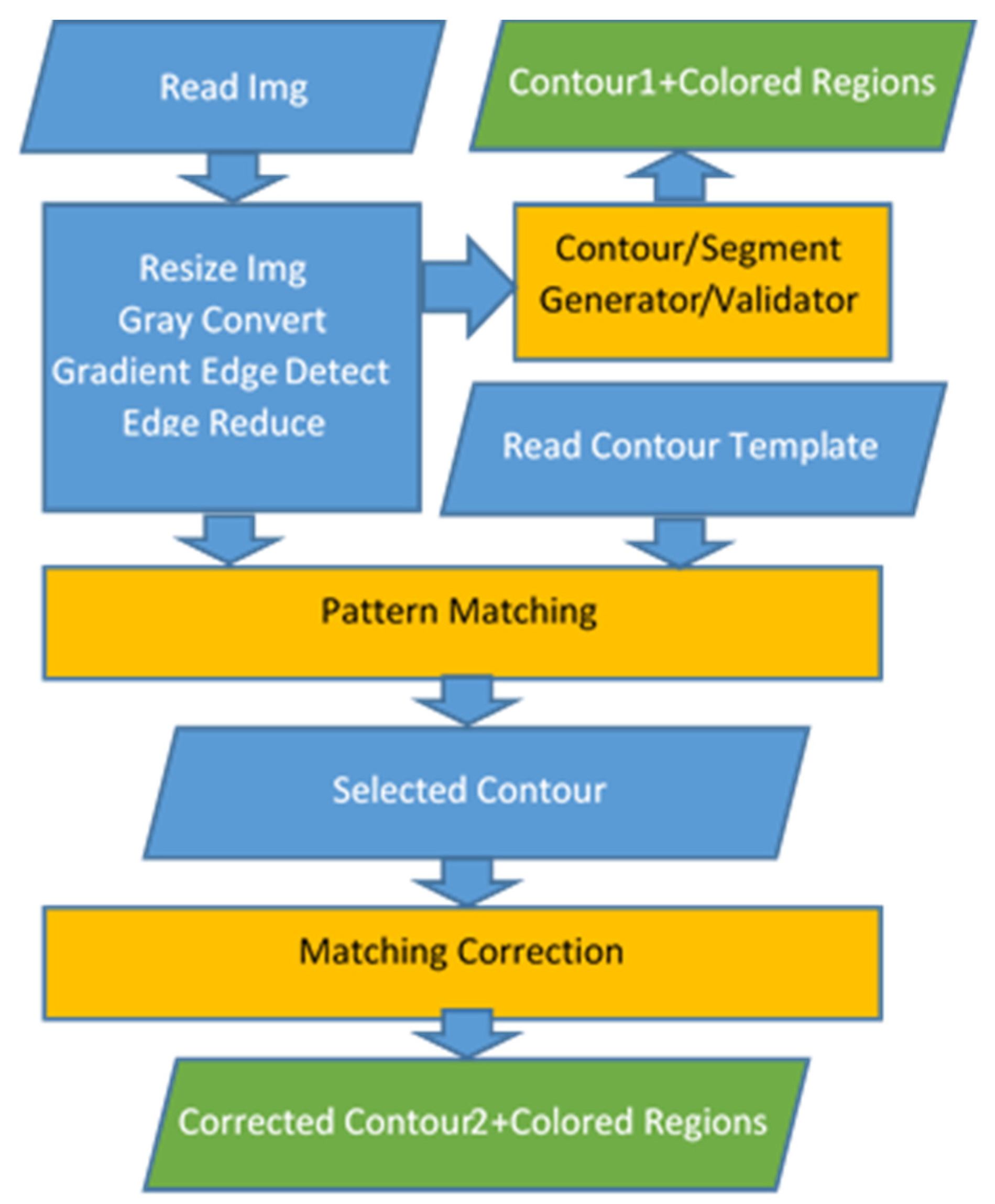
The first approach in the estimation of the fish’s morphological features was based on image processing techniques, and the steps of this technique are shown in
Figure 1. Octave-forge Image package functions were used to read and write images and then resize and convert them into gray scale, rotate them and perform pattern matching. Most of the Octave Image package functions used were compatible with the corresponding OpenCV library routines; thus, portability to other platforms was guaranteed. As a first step, the initial image was read and resized to the supported resolution (80 rows, 160 columns). The specific resolution adaptation was necessary in order to avoid undesired overlapping with the patterns that would be tested for matching. The image was converted into gray scale for edge extraction.
The discontinuities of the image corresponded to the edges of the objects appearing in the image. We desired to select the edges that corresponded to the contour of the fish in order to match an appropriate pattern template. Both coarse algorithms, such as the Sobel algorithm [
27] and more sensitive ones (e.g., Canny [
28]) were tested. Canny is based on frame-level statistics, and it is more accurate than Sobel but has higher complexity and latency. Experimental results showed that a finer edge detection algorithm such as Canny confused the adopted pattern matching algorithm, which often selected the wrong patterns with the wrong size, rotation and orientation.
A custom edge detection algorithm that takes advantage of the “imgradient” function of the Octave-forge Image package was developed, offering higher accuracy than Sobel but not the confusing detail of Canny. It is described in Algorithm 1. The “imgradient” function returns the gradient magnitude and direction associated with each pixel (in the matrices
gm and
gd, respectively). If the gradient magnitude of a pixel exceeds a high threshold (
magn_limit1), the pixel is assumed to belong to an edge; otherwise, a change in the vertical gradient direction is examined. If the gradient direction between adjacent vertical pixels seems to be reversed, and the gradient magnitude is above a second lower threshold,
magn_limit2 (average magnitude ≪
magn_limit2 ≪
magn_limit1), then the pixel is assumed to belong to the horizontal part of the fish contour. Horizontal gradient direction changes are intentionally ignored in order to avoid the detection of edges belonging to different objects. Since we assumed that the fish was at a horizontal alignment or with a slight inclination and never vertical, the largest part of the fish contour could be detected in this way, avoiding the detection of other irrelevant edges. This procedure corresponds to the gradient edge detect step of
Figure 1. Next, the mask displaying the detected edges (
edgesgm) is scanned again to remove isolated or small groups of pixels (noise). This is the edge reduce step in
Figure 1 that corresponds to step 18 of Algorithm 1.
| Algorithm 1 Custom edge detection algorithm |
gm, gd←imgradient(img);//get gradient magnitude/direction edgesgm←zeros with the same size as gm for i = 1 to rows(gm) for j = 1 to columns(gm) if img(i,j) is on the image borders continue; if gm(i,j) ≥ magn_limit1 //edge pixel if it corresponds to high gradient magnitude edgesgm(i,j)←1; else if gd(i,j)*gd(i + 1,j) < 0 if (gd(i,j), gd(i + 1,j) within angle limits) AND (gm(i,j) > magn_limit2) //gradient changed direction vertically and gradient //magnitude higher than magn_limit2 edgesgm(i,j)←1; else edgesgm(i,j)←0; Scan edgesgm and remove pixel islands with less than min_pix adjacent edge pixels
|
The first image processing approach toward the estimation of the fish contour and the localization of the fish parts exploits the
edgesgm image produced after the edge detection step, as described in the previous paragraph. This approach is in the path that leads to the “Contour1” output in
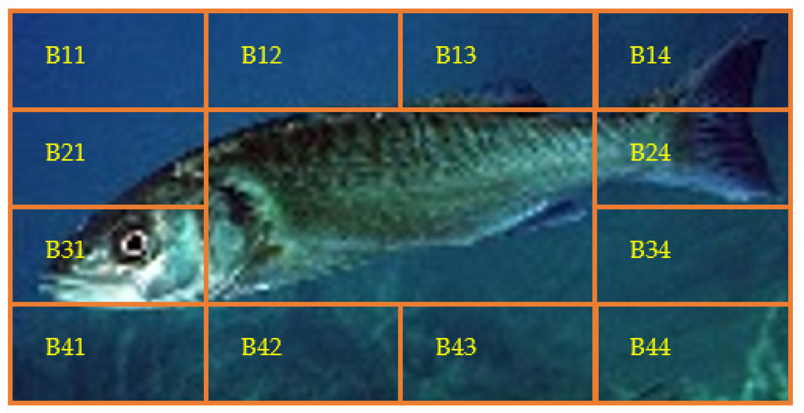
Figure 1. This path has low latency but produces valid results only if the background is simple (e.g., sea water). The system can validate whether this approach can be successfully followed using an image segmentation such as the one shown in
Figure 2. Taking into consideration that the resolution of the resized images was 80 × 160 pixels, the size of each one of the segments shown in
Figure 2, was 20 × 40 pixels. Assuming that the fish did not extend to the whole picture, it was expected that in most of the border segments B11-B21-B31-B41-B42-B43-B44-B34-B24-B14-B13-B12, the number of edges was small, unless the background was complex. The number of unconnected edges and the mean pixel value in each segment were estimated from the
edgesgm matrix. Remember that a pixel in the
edgesgm binary mask is one if it belongs to an edge, and it is 0 otherwise. If the number of disjointed edges in each segment was less than 10 and the mean pixel value in this segment was lower than 0.25, the segment was considered “empty” of edges; otherwise, it was characterized as “crowded”. An image displaying a fish with a simple background was expected to have a small number of crowded boundary segments, since only the boundary segments that contained a fish part would be crowded. If less than 6 segments were found to be crowded, the system assumed that the path toward “Contour1” in
Figure 1 led to acceptable results.
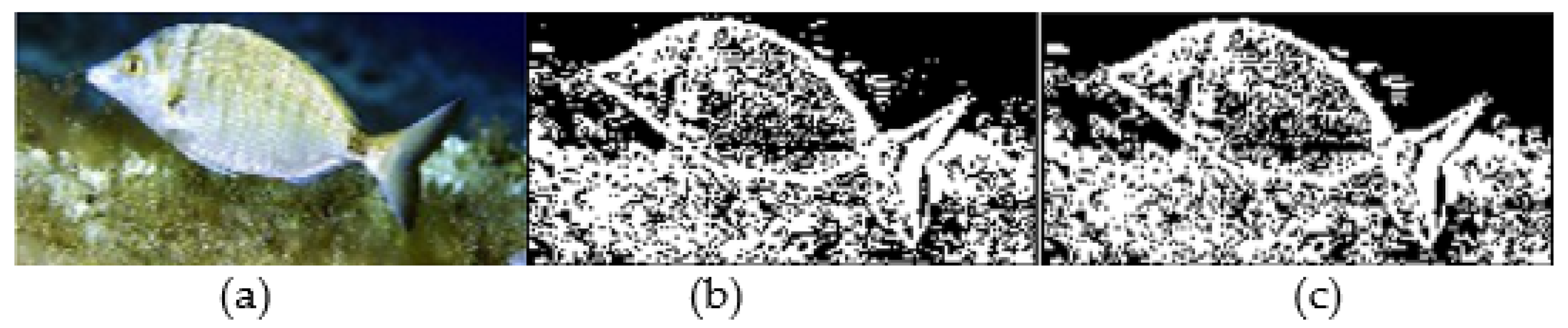
Figure 3 shows an example of an image that was rejected because 7 of the boundary segments were found to be crowded.
Once the system decides that the “Contour1” path in
Figure 1 is not acceptable, it attempts to determine the fish contour based on the edges found in the matrix
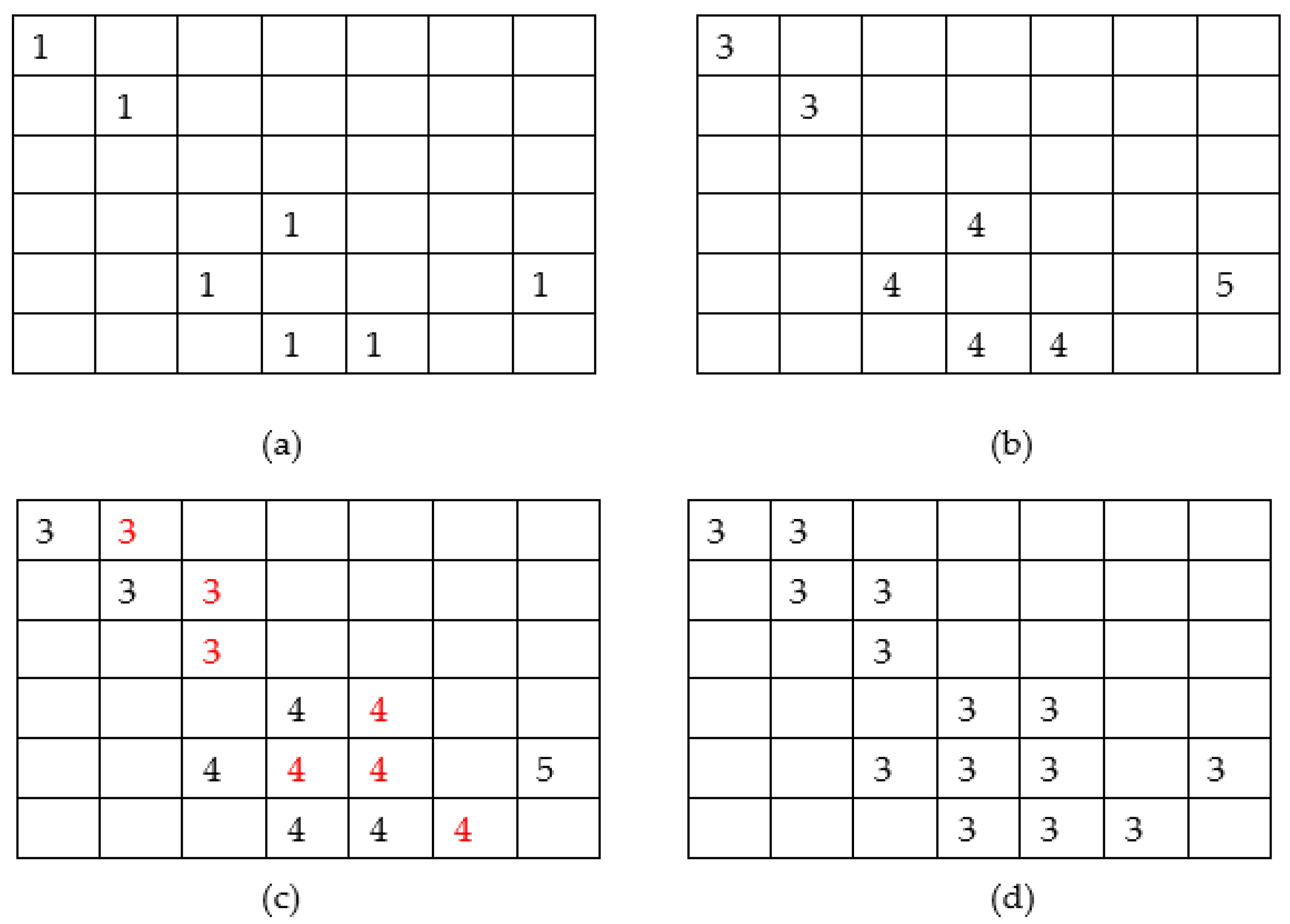
edgesgm. A connection of disjoint edges takes place as described in
Figure 4. In
Figure 4a, the contents of a part of the
edgesgm binary mask are displayed, assuming that the ones belong to the fish contour. A second matrix
edgesgm2 is constructed as follows. Each row (from top to the bottom) of
edgesgm is scanned from left to right. An identity
id is initialized to 0. All neighboring pixels are assigned with the same
id.
Figure 4b shows the form of
edgesgm2 after its construction. In order to connect the disjoint edges, the matrices
edgesgm and
edgesgm2 are scanned again. If 1 is found in the pixel (
i,j) of
edgesgm, the corresponding pixel in the
edgesgm2 matrix is set to
id if one of the pixels (
i − 1,
j − 1), (
i,
j − 1) in
edgesgm2 is already set to
id. If none of these pixels have been set to a non-zero
id, then the maximum value of
id is increased by 1 and this value is assigned to
edgesgm2(
i,
j).
Figure 4c shows the matrix
edgesgm2 after this step. As can be seen from this figure, the edges have been connected and thickened. To avoid having adjacent pixels with different identities in
edgesgm2, a third scan takes place to merge neighboring identities (
Figure 4d). After this merging process, the larger identity value corresponds to the number of disjoint edges. The larger edge (i.e., the one that contains the larger number of pixels) is selected as the contour of the bigger fish that is displayed in the photograph. In this way, although multiple fish can exist in the image, the analysis will proceed with the largest one. Complicated shapes in the body of the fish may confuse the proposed method. Consequently, a solid representation of the fish is generated by setting to 1 all the pixels within the (assumed) fish contour. The border of this solid fish body is now used as the fish contour in the pattern matching.
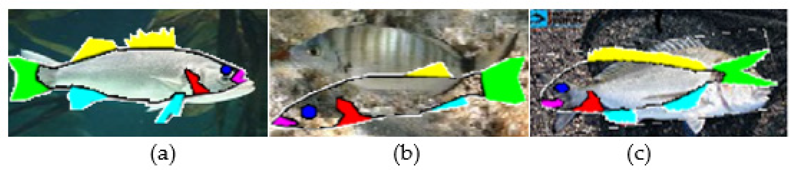
In order to determine the points that mark the borders of the fish parts, the fish contour is walked pixel by pixel, registering the corners (detected from direction changes) as landmarks. Using the morphology around the left and the right limits of the contour, the system recognizes the orientation of the fish. The location of the fish mouth can be easily determined in this case. On the opposite side, the area of the caudal fin is determined from the first corners of the upper and the lower part of the fish contour. For example, if the fish faces left, its mouth is at the point (
i,j) on the contour with the lower j (pixel (0,0) is the upper left corner of the image). The line connecting the rightmost corners of the upper and lower part of the contour is used to delimit the caudal fin. The other corners of the upper and lower parts of the contour can be used to determine the position of the spiny or soft dorsal fins and the anal or pelvic fins, respectively. For example, three consequent corners may indicate the start, peak and the end of a fin. The line connecting the start and the end corner in conjunction with the fish contour delimit the fin.
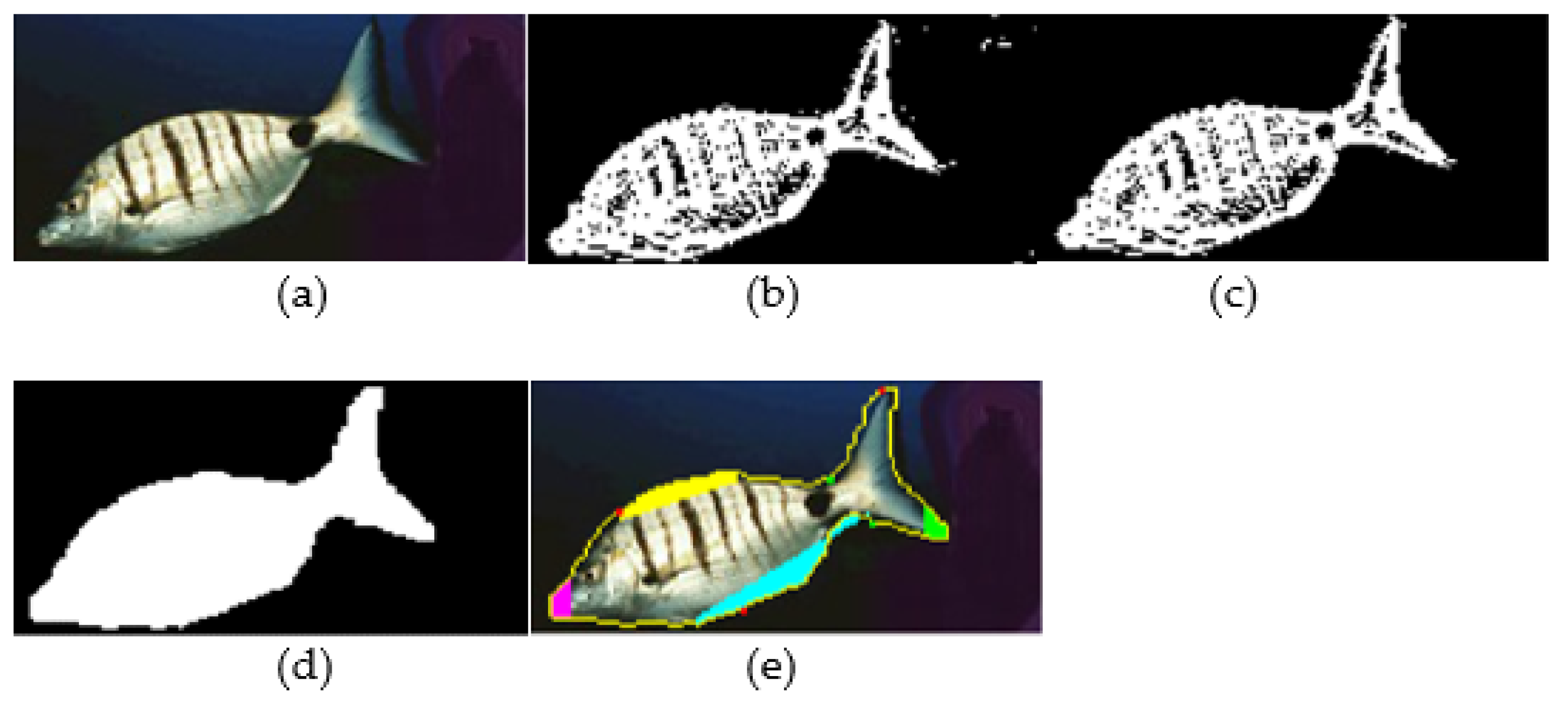
Figure 5 shows an example of a fish image processed with this approach.
Figure 5a is the original photograph. When the edges are detected using Algorithm 1, the
edgesegm matrix representation is shown in
Figure 5b.
Figure 5c shows the
edgesegm matrix after the edge reduction step that removes small islands of edge pixels that are considered to be noise. In
Figure 5d, the fish body was filled as explained earlier. Finally, in
Figure 5e, the recognized fish parts are colored: the mouth with pink, the spiny and soft dorsal fins with yellow, the pelvic and anal fins with light blue and the caudal fin with green. As can be seen from
Figure 5e, the caudal fin was partially recognized due to the orientation of the fish not allowing the proper determination of the upper corner.
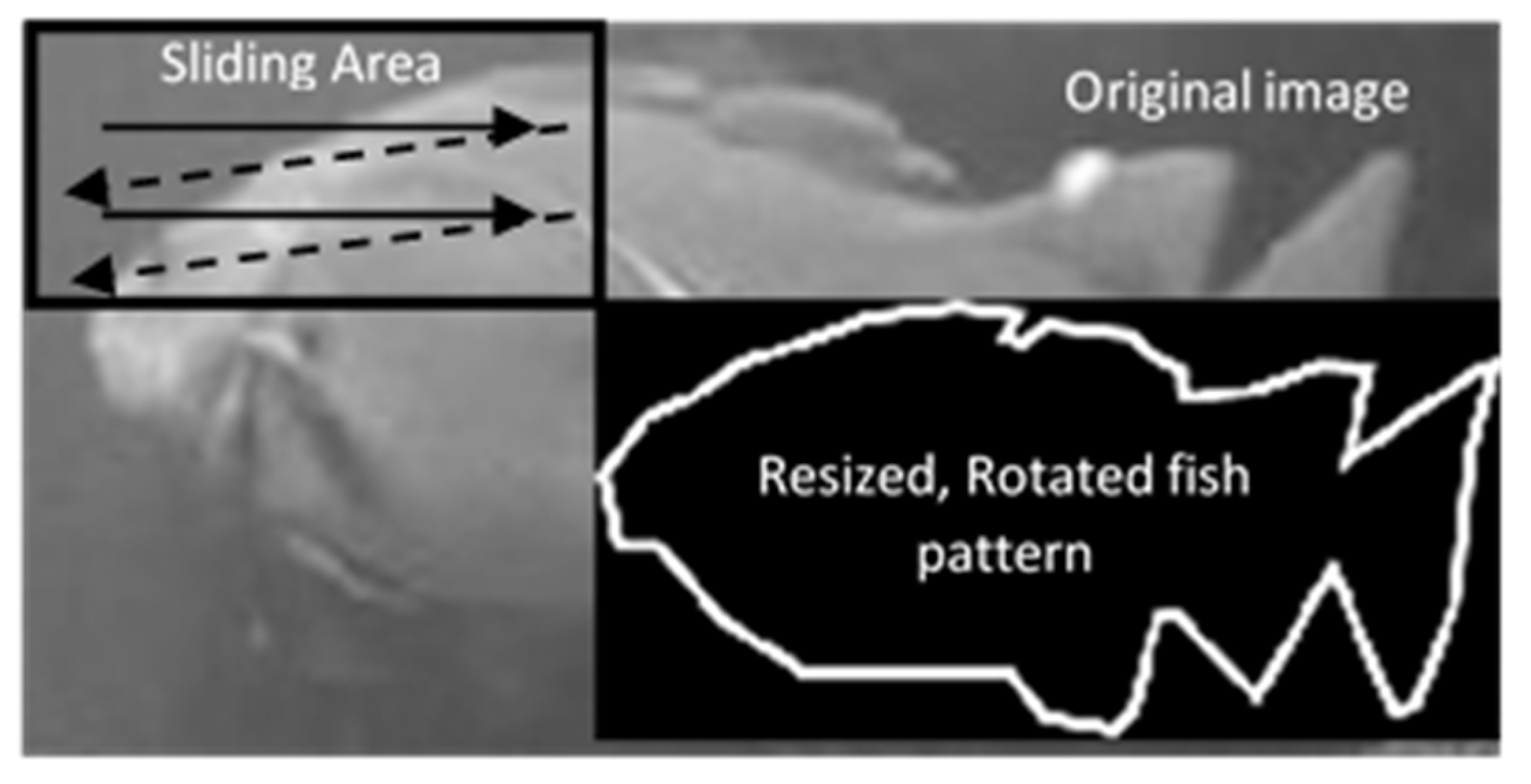
If the “Contour1” flow is unacceptable for a specific image, the pattern-matching path that leads to “Contour2” of the image processing approach can be followed. This method can be applied to images with more complicated backgrounds and attempts to match a contour pattern with the largest fish displayed. Algorithm 2 describes the Contour2 path, and it is used for every fish pattern
ptrn that has to be tested. The external loops (lines 3 and 4 of Algorithm 2) modify the input
ptrn by resizing (at line 7) and rotating it (at step 8) using the predefined strides
sscl and
sφ, respectively. Small strides can increase the accuracy, but they also increase the latency. The next step would be to slide the scaled and rotated fish pattern
ptrn3 at the allowed positions of
edgesgm as shown in
Figure 6. In each position (
r,c) of the
ptrn3 within
edgesgm, the correlation score
Sc is estimated as
| Algorithm 2 Pattern matching algorithm for the Contour2 approach |
Read ptrn best_score = 0; for scl = 1 to M with step sscl for rot = −φ to +φ with step sφ w = width(ptrn)-(scl-1)*2 h = height(ptrn)-(scl-1) ptrn2 = resize(ptrn,w,h) ptrn3 = rotate(ptrn2,rot) cc = normxcorr2 (ptrn3, edgesgm) Select (r,c) = max(cc) where (r,c) compatible with the edgesgm dimensions Sc = correlation of window centered at (r,c) if Sc > best score best score = Sc best rot = rot best scl = scl best r = r best c = c
|
The configuration (parameters
rot,
scl,
r and
c) that achieved the best score were selected for the specific pattern
ptrn. Sliding the resized and rotated pattern in successive (
r,
c) positions for the estimation of the correlation score using Equation (1) could be automatically performed with the
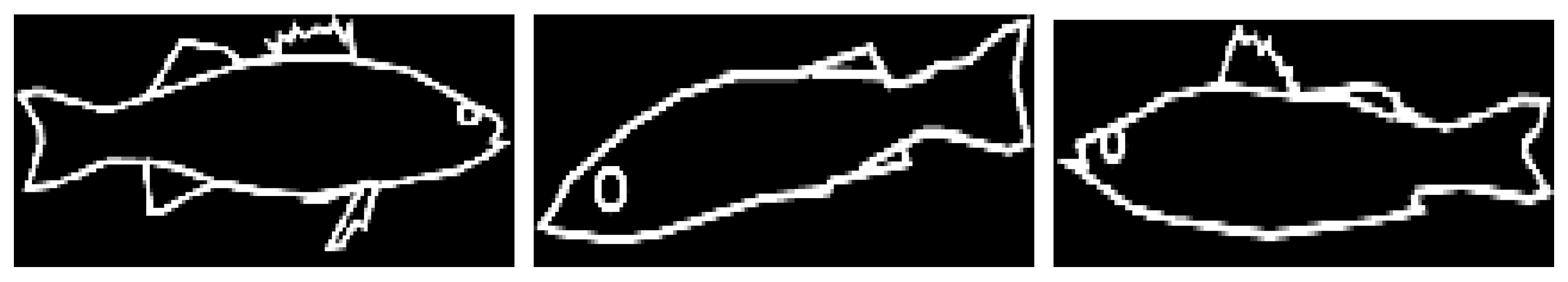
normxcorr2 function in the Octave Image package (Algorithm 2). The same procedure was repeated for all the patterns of the specific fish species. If the fish species displayed in the tested image was not known a priori, all the supported patterns
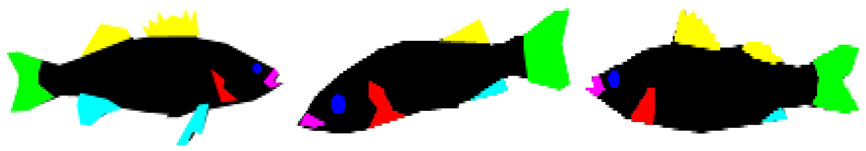
T had to be tested. In our case, where 25 images were used from each species, 3 patterns were representative for each species, and their horizontal mirror patterns were also used. For example, the 3 patterns used for sea bass are shown in
Figure 7. The corresponding patterns with colored parts appear in
Figure 8, since there was no need to use landmarks to delimit these parts in the Contour2 flow. As can be seen from
Figure 7 and
Figure 8, the set of fish patterns could be extended with already-rotated or slanted patterns (as is the one in the middle of
Figure 7). The actual fish dimensions were already known for a specific pattern, scaling and rotation.
It is obvious that the latency of the Contour2 flow depends on the number of patterns and the different scaling and rotation values tested. The number of different
Sc scores (
Nt) that have to be estimated are
where
Smax is the maximum scaling factor and the rotation angle of the pattern ranges between −
φ and +
φ, while
strd and
sφ are the scaling and angle stride, respectively.
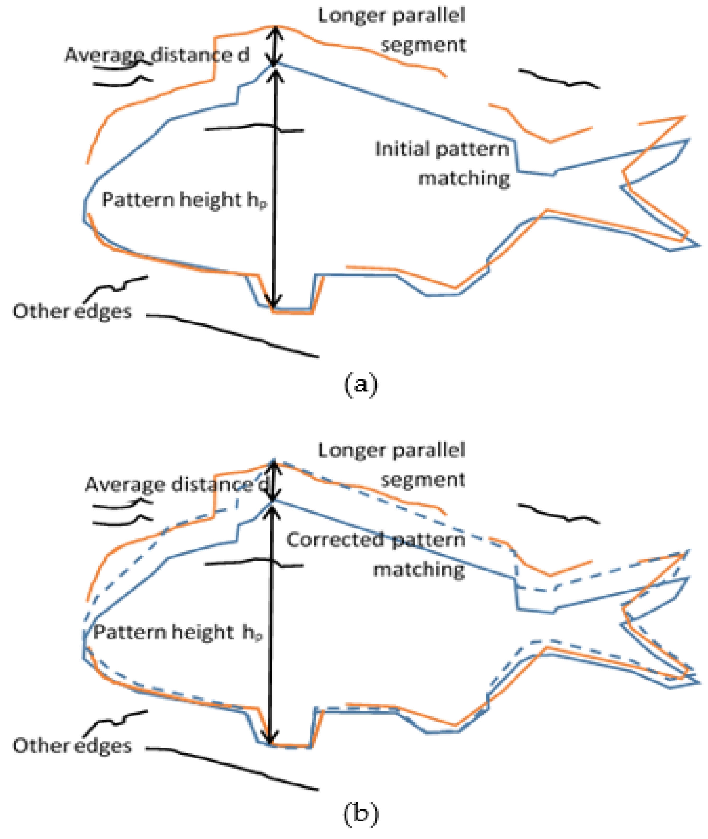
After the contour selection, the matching correction step shown in
Figure 1 takes place. The matching correction procedure is described using the example of
Figure 9, where the selected contour pattern (blue line) mainly matches the lower part of the fish (red edge segments). However, the resized pattern used failed to match the upper contour of the fish. The matching correction step examines the unmatched edge segments in the
edgesgm mask in order to find the one with the maximum length that is parallel with a part of the pattern contour. The parallelism score in the vertical or horizontal direction
Ps is defined as
Let us assume that an unmatched segment is examined for vertical parallelism with the contour, as is the case in
Figure 9. The Euclidean distance |
pk-ck| between each pixel
pk of the unmatched segment and the pixel
ck of the contour in the same column is estimated. The parallelism score
Ps is the number of pixels that have a Euclidean distance within the range (
d − ε,
d + ε). In the same way, a segment can be examined for horizontal parallelism if
pk and
ck are in the same row. If a long edge segment has an acceptable
Ps grade, the matching correction process will stretch the contour pattern in the corresponding direction to match this external segment. More specifically, in the case of
Figure 9, if the height of the initial contour pattern is
hp, and the average distance of the external edge segment is
d, the contour pattern will be resized to an overall height equal to
hp +
d (
Figure 9b). The corresponding fish pattern with colored parts (
Figure 8) will also be resized in the same way to localize the fish parts more accurately without using landmarks in the way they were used in the Contour1 flow. However, corners and landmarks have to be determined for the estimation of the fish length and height. Examples of Contour2 flow output images are shown in
Figure 10.
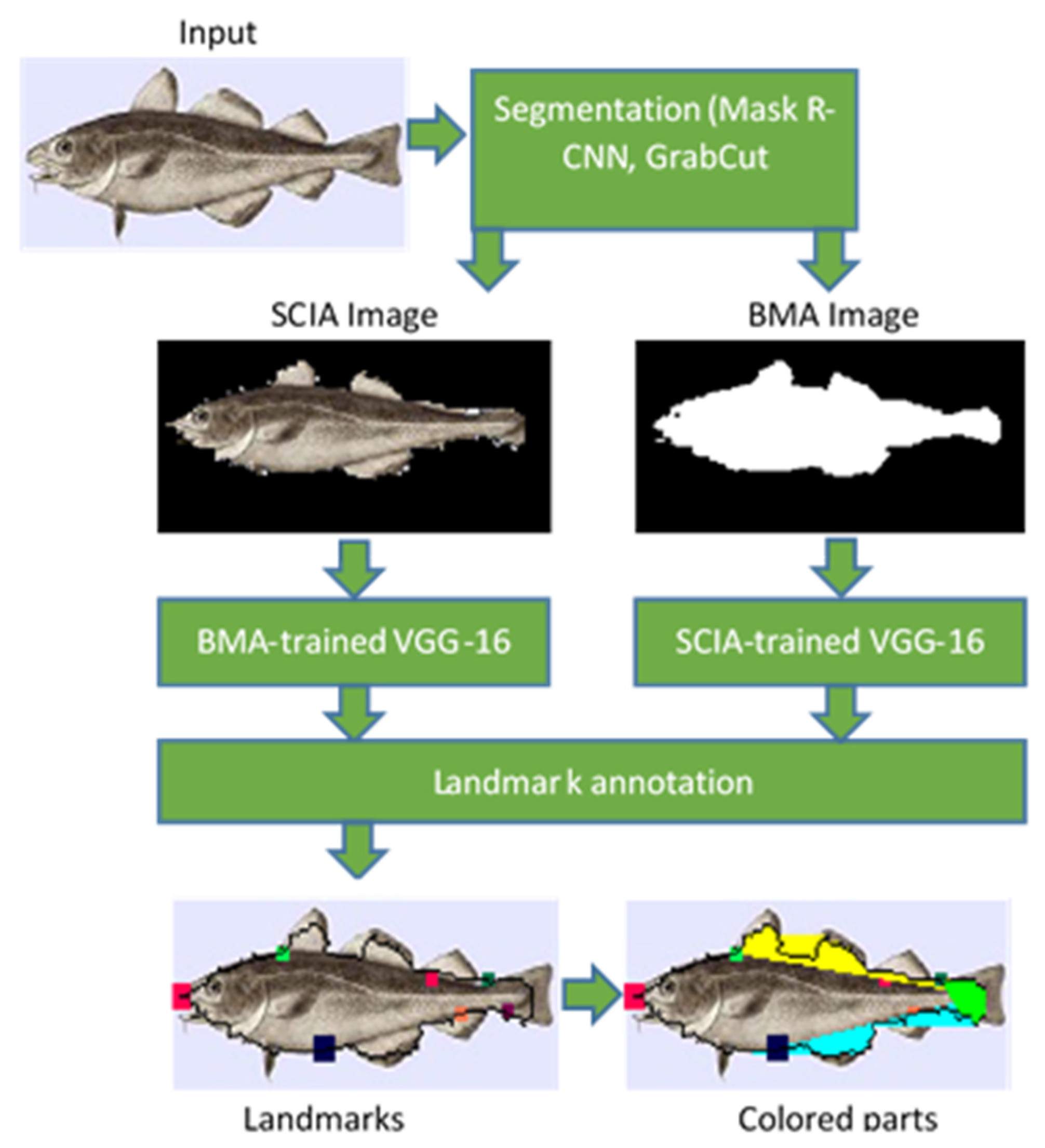
2.3. BMA and SCIA Deep Learning Approaches
The steps followed in the deep learning approaches are shown in
Figure 11. The input image is initially segmented based on the method described in [
29]. The bounding box and the pixel-wise segmentation mask of all the recognized objects in the image are predicted using a mask region-based convolutional neural network (Mask R-CNN). It has to be noted that multiple objects can be recognized with different confidence levels. The largest fish will be recognized with higher confidence, while smaller or slanted or obscured fishes can also be recognized with lower confidence if the system is trained appropriately. In the current version, only the object with the highest confidence level is further processed. As was already mentioned in
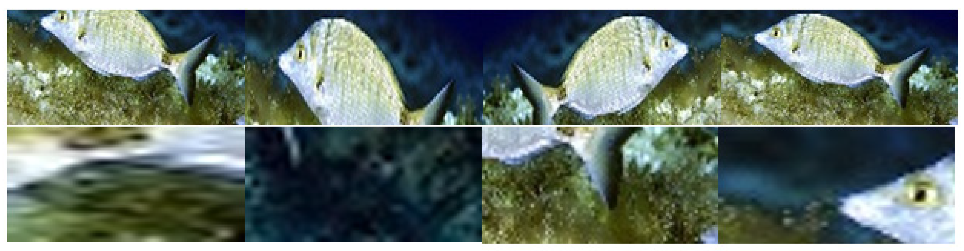
Section 2.1, the initial dataset consisting of 25 photographs or species is augmented by mirroring or cropping the initial images and applying jitter in order to generate multiple images from a single image. The resulting images are assumed to display a fish if less than 20% of the fish has been excluded from the cropped image (
Figure 12). A higher threshold can be used if the obscured fish have to be recognized.
The Mask R-CNN was introduced in [
30] as a successor of the Faster R-CNN. A binary mask output is added to the class name and bounding box output of the Faster R-CNN. The Mask R-CNN adds a fully connected CNN on top of the Faster R-CNN features. The backbone architectures employed in the Mask R-CNN are ResNet and ResNeXt of depths of 50 or 101 layers, respectively [
30]. As shown in [
29], the segmentation of the Mask R-CNN is not very precise, since regions that do not belong to the object are included in the output mask. Therefore, the GrabCut algorithm [
24] was employed to improve the segmentation of the object that was recognized by the Mask R-CNN. However, GrabCut, in its attempt to exclude non-fish regions, may also exclude fish parts from the mask. None of the two approaches (individual Mask R-CNN or Mask R-CNN with GrabCut) can perform perfect contour detection. Therefore, OpenCV implementation of the GrabCut algorithm was used. The Mask R-CNN was pretrained with the COCO data set [
31]. The COCO dataset contains 80 object categories and more than 120,000 images, but no fish species. However, it can segment fish objects in a satisfactory way, even if it does not recognize the displayed fishes. Alternative segmentation methods such as U-Net [
32] could have been employed. U-Net can be trained on small data sets, and it is appealing for mobile implementations since it requires a small number of resources. Recent U-Net approaches [
33,
34,
35] further improved the speed, the model and the training dataset size. U-Net has been tested mainly on medical imaging, and for this reason, a more general architecture (Mask R-CNN) was employed here.
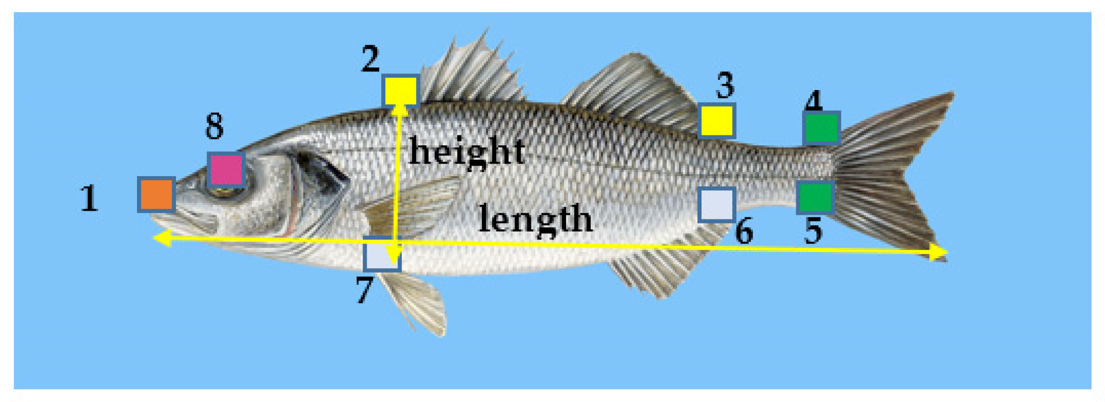
In the training procedure, 8 landmarks that were common to the four fish species studied here were annotated either on the binary mask (binary mask annotation (BMA)) or on the segmented colored image after subtracting the background (segmented color image annotation (SCIA)). The landmarks used in the deep learning approach are shown in
Figure 13. Landmark 1 determined the position of the mouth. The pairs of landmarks (2,3), (4,5) and (6,7) determined the limits of the fins at the top (spiny and soft dorsal), the caudal fin and the fins at the bottom (anal and pelvic). Landmark 9 corresponded to the position of the eye, but it could not be determined accurately with the specific dataset size. The fish body height was defined as the Euclidean distance between landmarks 2 and 7. The fish body length was defined as the Euclidean distance between the mouth landmark (landmark 1) and the position of the farthest contour pixel on the opposite side (caudal fin).
New datasets were formed from the BMA or SCIA masks, along with the annotated landmarks. These datasets were used for the training of a VGG16 CNN using Keras and Tensorflow. The VGG16 CNN was trained to generate the 8 pairs of coordinates of the fish landmarks shown in
Figure 13. The VGG16 CNN architecture that was already trained on ImageNet [
25] was employed in the transfer learning method that followed. The fully connected head layer of the VGG16 model was removed. The weights in all other layers were frozen, and a new fully connected layer head was constructed with 8 pairs of landmark coordinates as the output. During the additional training process followed to train the new head layer, the estimated landmarks were compared with the ground truth landmarks annotated on the SCIA image. The weights of the new head layer were determined using mean squared error (MSE) loss and the Adam optimizer.
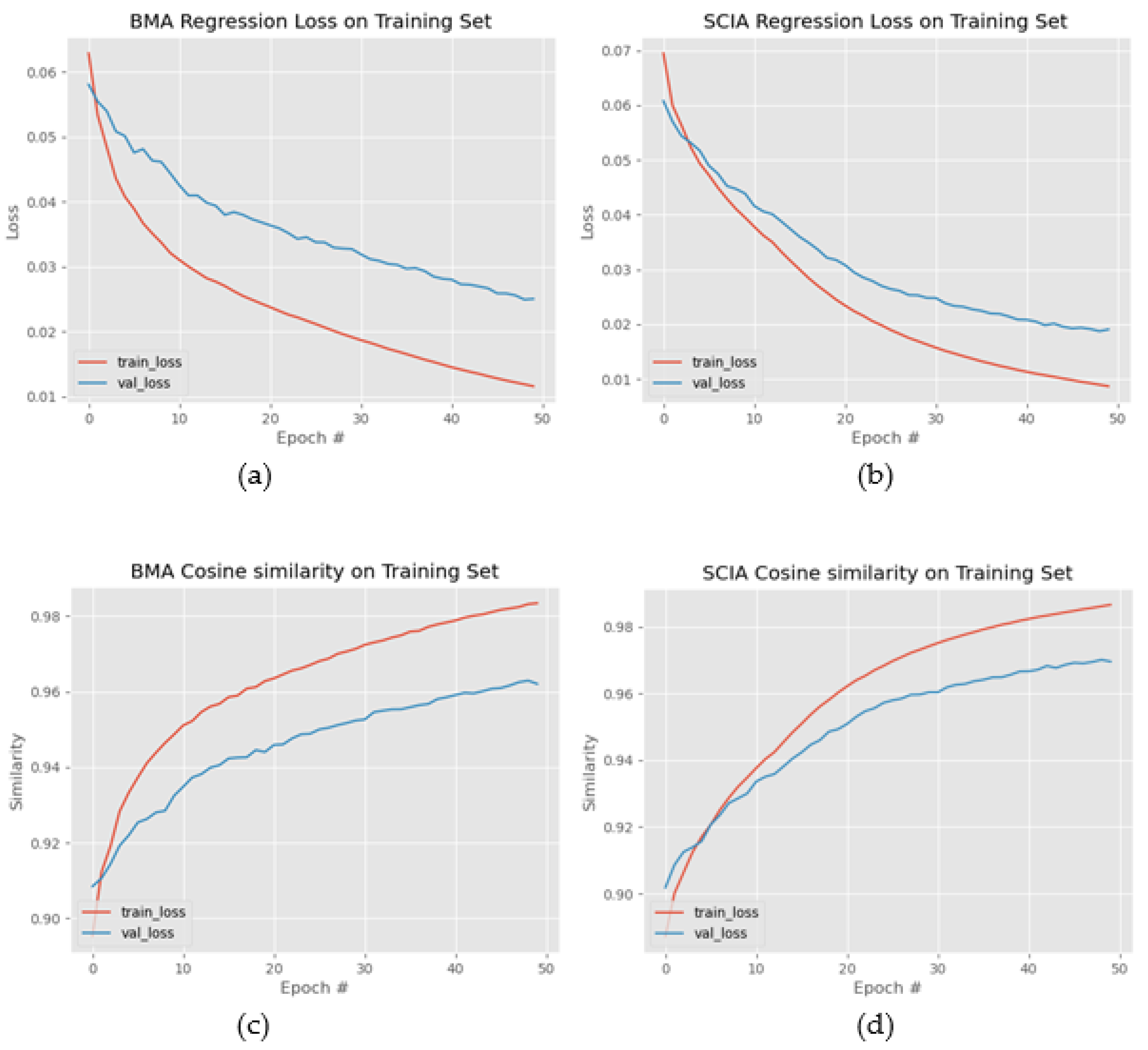
The regression loss of the training and the validation set for the BMA and the SCIA datasets are drawn in
Figure 14a,b, respectively. Fifty (50) epochs were sufficient for flattening the regression loss curves; thus, the training could be terminated after 50 epochs for the specific dataset to avoid overfitting. The cosine similarity was also employed in
Figure 14c,d in order to measure the alignment of the predicted positions with the true landmark positions. The cosine similarity of two non-zero vectors
V1 and
V2 was estimated as
, where “·” denotes the dot product. Cosine similarity values +1, −1 and 0 corresponded to the fully aligned, opposite or orthogonal vectors, respectively.
The VGG16 CNN was used for object detection and landmark annotation on a test image [
32]. The fish contour was determined from the binary mask that was generated by the Mask R-CNN. The annotated landmarks were used to measure the fish dimensions (length and height) and to delimit the fish parts of interest (i.e., the caudal fin, the spiny and soft dorsal fins, the anal and pelvic fins and the mouth). The aforementioned procedure (training and testing) was implemented in Python. The distances were calculated, and the contour, the landmarks and the colored fish parts were available in the output image of this approach, as shown in
Figure 15.
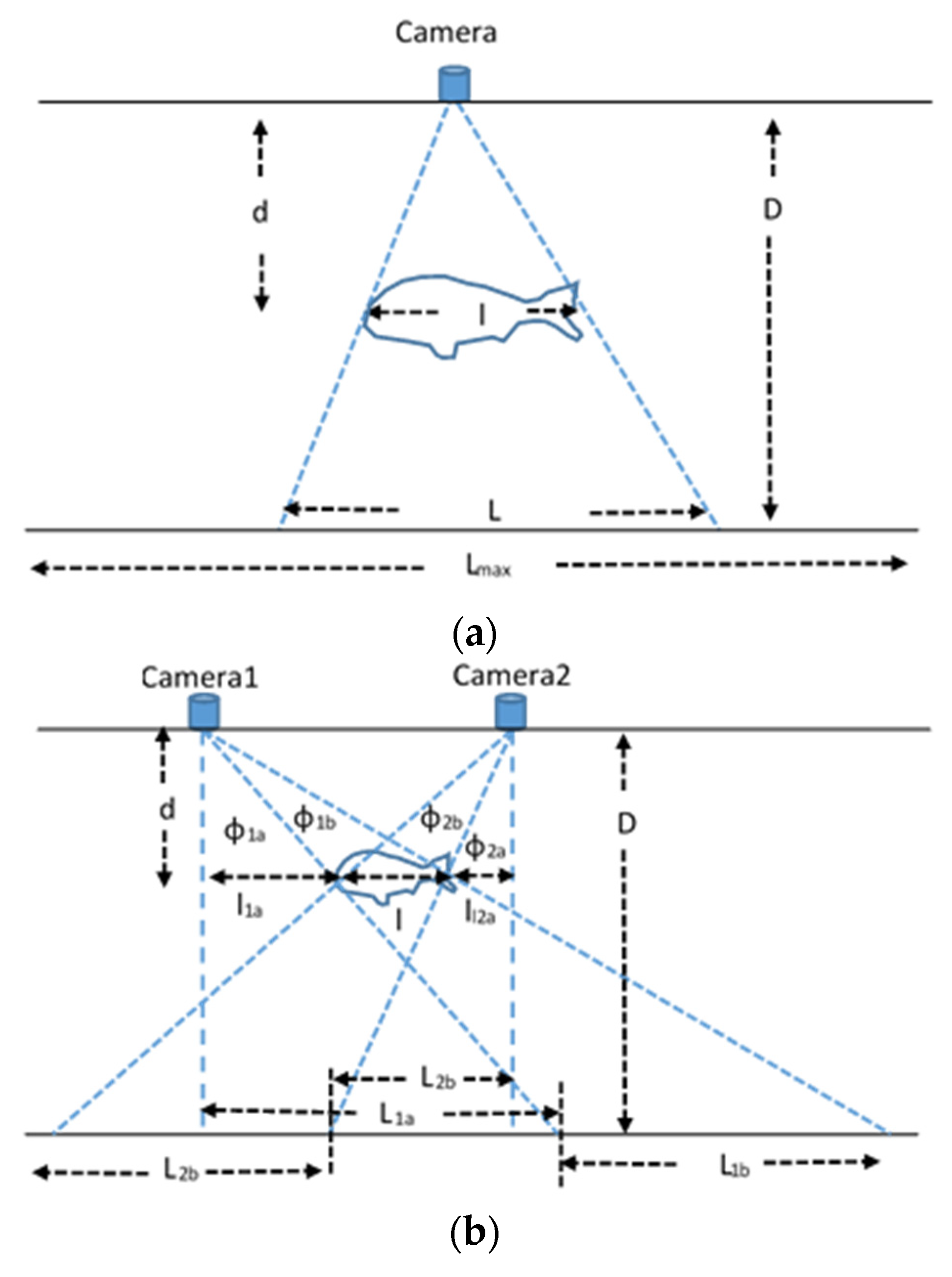
2.4. Estimation of Absolute Dimensions
A single camera could not be used to estimate the absolute dimensions of a fish or any other object unless its distance from the object was known. In some cases, this is feasible (e.g., in intrusive methods that require the fish to be taken out of the tank and placed on a table in order to measure its length and weight). Instead of measuring these dimensions manually, a camera placed in a constant position and at a known distance from the fish could be used to estimate automatically the required features, as shown in
Figure 16a. In this figure, the camera is facing a bench or a wall, which is denoted by the bottom horizontal line. Let us assume that the camera field of view can display the
Lmax length of the bench and the corresponding number of pixels in this direction is
Pmax. The distance of the camera from the bench is
D. If the fish was at this exact distance from the camera, and its length
L corresponded to
P pixels, then
If the fish is at a known distance
d, its actual length
l can be scaled as follows:
This way of measuring the fish length could also be applied if the image was captured when the fish entered a narrow fishway, as described in [
5]. If the fish distance was not known, then stereoscopic vision could be applied using a pair of cameras. In [
6,
16], popular methods based on epipolar planes were described for measuring absolute fish dimensions. Moreover, in [
7], affine transformations were applied to adapt the shapes of fish that were photographed from an angle. A slightly different modeling than epipolar planes is described here. The modeling concerns the case where the fish is assumed to be parallel with the background wall or bench, and its length is measured at an unknown distance
d as shown in
Figure 16b.
From the view of each individual camera, the distances concerning the projection of the fish on the background bench (
L1a,
L1b,
L2a,
L2b) can be estimated using Equation (4). Knowing these parameters and the distance
D of the cameras from the background wall, the angles
φ1a,
φ1b,
φ2a and
φ2b can be estimated as follows:
Now, assuming that the angles
φ are already known, we also estimate the tangents at the distance
d of the fish, and we also take into consideration that the distance
LC from the cameras is known:
From Equations (10)–(14), the parameters
d,
l1a,
l and
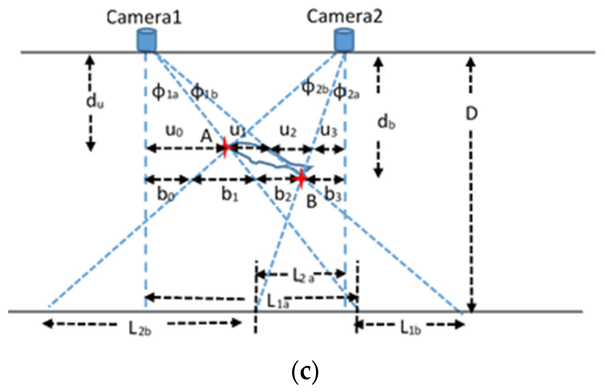
l2a can be calculated. Using a similar approach, the length of a slanted fish can also be estimated as shown in
Figure 16c. In this figure, the length of the fish is the Euclidean distance between points A and B. The positions of points A and B can be determined if the pairs of distances (
du,
u0) and (
db,
b3) are known, respectively. Assuming again that
L1a,
L1b,
L2a and
L2b have been estimated using Equation (4), the five pairs of equations that will lead to the determination of the positions of points A and B are the following:


