Algorithm for Designing Reconfigurable Equipment to Enable Industry 4.0 and Circular Economy-Driven Manufacturing Systems

Abstract

In the paradigm of industry 4.0, manufacturing enterprises need a high level of agility to adapt fast and with low costs to small batches of diversified products. They also need to reduce the environmental impact and adopt the paradigm of the circular economy. In the configuration space defined by this duality, manufacturing systems must embed a high level of reconfigurability at the level of their equipment. Finding the most appropriate concept of each reconfigurable equipment that composes an eco-smart manufacturing system is challenging because every system is unique in the context of an enterprise’s business model and technological focus. To reduce the entropy and to minimize the loss function in the design process of reconfigurable equipment, an evolutionary algorithm is proposed in this paper. It combines the particle swarm optimization (PSO) method with the theory of inventive problem-solving (TRIZ) to systematically guide the creative potential of design engineers towards the definition of the optimal concept over equipment’s lifecycle: what and when you need, no more, no less. The algorithm reduces the number of iterations in designing the optimal solution. An example for configuration design of a reconfigurable machine tool with adjustable functionality is included to demonstrate the effectiveness of the proposed algorithm.

1. Introduction

The fourth industrial revolution, coined in some areas as industry 4.0, aims to transform the manufacturing industry by adopting large-scale industrial-IoT, edge-cloud computing and supporting technologies (industrial cybersecurity, machine learning, deep learning, and data analytics) to increase predictability, connectivity within the supply and value chains, agility, as well as capacity to optimize processes, such as to face with an increased market dynamics and granularity of market requirements [1]. The circular economy, in symbiosis with industry 4.0, aims to transform the manufacturing industry into a more sustainable one from economic, ecologic, and social points of view by changing the paradigm in which business models and offers are designed, developed, produced, delivered, consumed, and withdrawn [2]. Value optimization, lifecycle thinking, eco-innovation, stewardship, transparency and traceability, system thinking, and tight collaboration in the value chains are key principles of the circular economy [3]. For the manufacturing industry, circular economy pushes practices towards product-service systems [4] and servitization [5], as well as towards consideration of the 6R closed-loop for sustainable manufacturing: reduce–recover–remanufacture–recycle–redesign–reuse [6]. Combining industry 4.0 with the circular economy and with efficient use of workforce and machines, we reach the paradigm of industry 5.0 [7,8]. Industry 5.0-driven manufacturing systems must embed high agility and adaptability for mass customization of products [9].

Beyond any necessary transformations of processes in terms of digitalization and data-driven business models, clean production, and mechanisms for recovery, recycling, and reuse of products, consideration of lifecycle and lifetime perspectives in close connection with servitization and mass customization requires, with no reservation, embedded capabilities of reconfigurability in the manufacturing systems and associated equipment to fulfill the goals of industry 5.0.

Reconfigurability at the machine level is about modularity, convertibility, personalized flexibility, scalability, diagnosability, integrability [10,11]. By comprising these capabilities, a reconfigurable machine tool from a manufacturing system is aligned to industry 4.0, circular economy, and smart workforce requirements. Thus it is aligned to the paradigm of industry 5.0, also coined as intelligent manufacturing ecosystem [7].

Nevertheless, reconfigurability comes with an increased entropy in design. Therefore, it is crucial for tackling the design process of reconfigurable equipment in the context of a given manufacturing capacity to align it to the guiding principles of industry 5.0. The major challenge is the necessity to handle the mix of objective functions (also named target functions) that frames reconfigurable equipment.

Modularity is achieved by the ability of the independent, intelligent equipment to cooperate and act as a compact unit [12]. Scalability is reached using the communication protocol where theoretically, an unlimited number of high and low priority equipment could be connected [12]. Convertibility and customization are accomplished at a certain level by the ability to configure on request and in real time the functionality of intelligent equipment [12]. Integrability is expressed by implementing solutions that ensure stability and compatibility between old and new hardware modules and software packages [12]. Diagnosability is the ability of the main control unit to gather information from the connected modules, identify incompatibilities, cancel commands to the concerned equipment, and alert the operator about the identified issues [12].

The key characteristics of reconfigurability are interconnected. In principle, a robust design requires tackling them concurrently. It is thus the purpose of this paper to focus the research investigation on a generic design algorithm that incorporates the potential to tackle simultaneously engineering key performance indicators (E-KPIs) that describe a complex design optimization function (note: here, reconfigurability).

In this respect, the next section of the paper provides a synthesis of design algorithms suitable for the purpose mentioned above. The investigation is not limited only to algorithms strictly dedicated to reconfigurable machine-tool design, even if this area is also included in our analysis. The reason is to explore contributions beyond the scope of reconfigurable design that could be useful also for this specific topic.

2. Research Focus and Relevance

The conceptual design of new complex products is a very challenging task [13]. Various modes that combine creative thinking with logical thinking during the whole process of product conceptualization are envisaged [14]. To handle the complexity of the product conceptualization process, early formulation of the space of intervention (design scope) is necessary [15]. Design boundaries, constraints, and priorities are defined in this respect [16,17]. Literature reveals a wide range of means and approaches proposed in this respect. It is usual nowadays to consider structured planning tools in the early stages of a design project for defining and quantifying the design problem [18]. Integrated systems of planning methods and methodologies help design engineers create relevant design information before conceptualizing new products [19,20,21]. Such frameworks provide data on expressed and latent market requirements [22], support ranking of design requirements and specifications [23,24,25], establish design targets [26,27], determine design priorities in a constrained space of intervention [28], as well as define both technological and economic constraints [27,29]. This information is input for the conceptual design phase [30,31].

An extensive pallet of approaches is reported in the literature to support the product conceptualization process (e.g., [19,30,32,33,34,35,36]). The individual and collective experience, creativity, and several other context-related factors contribute to the formulation and selection of the design framework for a given design problem [37,38,39,40]. Methods, methodologies, and technologies increase the chance of getting out reliable results [30,37,41]. Positive potentials in defining reliable solutions using conceptual design chains based on existent methods and design principles are analyzed and demonstrated by several works (e.g., [14,36,42,43]). Chaining of the design method is based on different approaches, which vary from physical laws to evolutionary algorithms (e.g., genetic algorithms [44], particle swarm intelligence [45], as well as other stochastic search techniques [35]). In principle, for various design problems, we need to select adequate design methods [46]. In this respect, [37] reveals the importance of having a knowledge-based chain for supporting conceptual design when engineers face multidisciplinary problems. They develop a platform for synthesizing and reusing known design principles and solutions to support this process. For ideas association during the dynamic process of product conceptualization, contributors in [38] propose a cognitive theory of role-playing for modeling the distributed interactions between actors involved in the ideation process and a linking model (DIM-2) of ideas shared in the group. This approach improves idea generation and selection by dynamically combining individual and collective contributions. In the same register of solution formulation, [39] highlights the importance of collaboration in conceptual design using various distributed platforms and means. Other studies, such as those reported by [30,47], demonstrate the importance of stimulating and managing human creativity in a structured framework during the conceptual design process for defining highly mature and original solutions.

It is important to highlight here that optimization in the conceptual phase should not be confused with dimensional optimization or multiobjective optimization, which is the field of traditional optimization theory and operates with quantitative parameters for an already given formulated concept or design [48]. Returning to our research subject, one can conclude that one specificity of the approaches mentioned in the above paragraphs is they mainly focus on qualitative improvements and less on concept optimization. However, many research reports show that the complexity revealed by most of the design problems makes identifying a global optimum solution of a concept impossible [16,17], with the goal of concept design being limited to improvement issues rather than quantitative optimization of design concepts [33,46]. Even if the quantitative optimization problems, in meeting multiple targets during the conceptual design phase, are difficult to achieve for complex design problems, defining solutions close to optimum is desirable. Therefore, various evolutionary algorithms have been developed and used to meet this goal [46]. When some partial solutions are formulated, these algorithms aim to automate at a certain extent the conceptualization process. Several works demonstrate this conduit. Some relevant references in this respect are further highlighted. For example, [41] uses functional reasoning and a pool of building blocks to conceptualize an engineering solution to a given design subject. Here, conceptualization is more based on combinations of predefined blocks to fit some boundaries, as in a puzzle, without inducing a creative input in this operation. Paper [49] uses particle swarm optimization (PSO) to define an optimal production equipment configuration using a limited set of modules from a library. The best local solution is thus obtained, but using a “frozen”, “mechanistic” space of intervention, in which no creative support of engineers is brought during solution formulation. In the same spirit, the work reported by [42] exploits genetic algorithms to handle this type of problem. Comparable evolutionary algorithms are considered by [43,50] that automate the conceptualization of a particular engineering design problem. In this register, the work conducted by [34] can also be reported. These algorithms run on a computer without human interaction in this process; thus, the optimization problem does not infuse any human input during the incremental product conceptualization process. This is a limitation because we reject from the algorithm an extremely valuable resource, the human expertise. Conceptually speaking, this rejection contradicts the core law of ideality highlighted in [32].

Despite the long history of engineering design, a conclusion coming up with clarity from the current developments in this field is that no universal framework and tool exists today as a “panacea” for tackling conceptual design [14,35]. Furthermore, there are still insignificant contributions and know-how in combining qualitative improvement/optimization with quantitative improvement/optimization in conceptual design. Nevertheless, throughout the product conceptualization process, many design problems require a balanced intercorrelation between qualitative optimization, led by structured creativity/innovation, and quantitative optimization, led by optimal design algorithms to efficiently direct design efforts towards highly effective solutions.

Narrowing the space of investigation to the design algorithms for reconfiguration, we can report that most of the cases focus on control algorithms or on reconfigurable manufacturing systems, and fewer are directed towards designing reconfigurable machine tools. Those related to reconfigurable machine tools put a clear emphasis on modularity; thus, being too sectorial for our research. Searching in Clarivate Analytics with the keyword “reconfigurable machine tool”, 128 references are displayed. Refining the search with the word “algorithm”, references are reduced to 21, from which only 5 papers introduce algorithms for reconfigurable machine-tool design. Searching in the Scopus database with the same combination of keywords, 25 papers are returned, from which only 1 paper is referring to reconfigurable machine-tool design and is new to those identified in Clarivate Analytics. The first work referenced here is [49]. It formulates a design problem by considering three conflicting parameters: configurability, cost, and process accuracy. This research is outside the scope of our focus because it does not treat reconfigurability from the perspective of its intrinsic characteristics and has nothing to do with the conceptual design of the reconfigurable machine tools. Nevertheless, it draws on the angle of applying the PSO algorithm to solve the multiobjective optimization problem, but in the register delimited by dimensional optimization [48]. In [51], the authors propose a framework for rapid design of the architectural layout of a reconfigurable machine tool. The focus is strict on modularity, which is only a secondary characteristic of reconfigurability, and consists of a step for layout configuration and a subsequent step of layout evaluation. This limitation places research from [51] outside the scope of the job investigated in this paper. Paper [52] also deals with design in the case of reconfigurable machine tools, but the focus is on a different design stage; that is, after the stage of configuration design, treating the problem of accuracy of the machine in the case of a new reconfiguration. Despite the value of this research, the design focus is not in the same area as the one indicated by our paper. As the case of [51], paper [53] also treats reconfigurable machine-tool design from the limited scope of modularity. It proposes an algorithm to define the minimum number of modules necessary for the machine to solve a given family of parts. It is more an algorithmic search for a minimum in a predefined space, which does not require an infusion of creativity, but rather a search in the space of possibilities. From this perspective, this work is also not related to the scope of research investigated in this paper. In [54], the research stays in the same register as the one in [53], dealing with minimization of modules changed when parts are changed. This is an important element in the reconfigurable machine-tool design but is mainly related to a single key performance indicator that optimizes modularity layout. Using tabu search algorithms, paper [55] operates with the same optimization problem of defining the optimal path for reconfiguring a machine tool. It is another way to solve the same problem investigated by [53,54]. The layout design of a reconfigurable machine tool starting from the space defined by the family of parts using metaheuristics is proposed in [56]. Even if the design problem remains in the register signaled by [53,54,55], this work has the merit of putting the design in a more concrete context—the lifecycle perspective of the parts that will be manufactured on that machine. This idea is also considered in our research. The last paper identified in the databases dealing with reconfigurable machine-tool design is [57]. It is about applying typical multiobjective optimization problems to measure machine reconfigurability from a modularity perspective and machine capability. It uses genetic algorithms to identify the non-dominated combinations and afterward a multicriteria method to rank Pareto frontiers. The topic of optimization is at the stage of design conceptualization where quantitative parameters are already known; thus, being possible to map the space of possibilities with a classical optimization formalism. The idea to take this aspect in an earlier phase of conceptualization is imported into our research.

Our literature survey led us to conclude that, even if many of the design algorithms have merits to be considered for the problem of reconfigurable machine-tool design, some limitations still exist, in the sense that they are too sectorial. In practice, the problem is a bit more complex than in the simplified spaces investigated by the reference papers.

These aspects motivated us to investigate new frontiers for knowledge creation and to propose an augmented design algorithm that simultaneously combines computer-driven evolutionary intelligence and human intelligence to formulate a mature solution to a problem. The thesis behind this proposal is that augmentation compensates drawbacks of both pure automatic algorithms that are suitable for implementation in a computer program and pure human judgment, which faces difficulties in dealing with the complexity. It tries to aggregate the strengths of the two sectoral approaches, such as to handle in a better way the underdefined and highly entropic space of ideation. Thus, this paper explores the space of engineering design by proposing a spiral approach that combines structured innovation and stochastic search algorithms to tackle the design of reconfigurable machine tools, but not only; the ambition is to propose an algorithm that can be expanded to other similar problems. The idea is to involve the creative potential of engineers at each iteration stage of the evolutionary algorithm and to direct this potential towards the most effective vectors of evolution. This means the design framework should be subject to the law of convergence [58] and the law of ideality [32]. The law of convergence states that a good design process leads to a mature solution for the problem under consideration after a small number of intermediary attempts (minimum possible iterations). The law of ideality strives for solutions that include as much as possible useful functions and as minimum as possible harmful functions (no harm at the limit).

The novel conceptual design method adapts the traditional PSO theory proposed in [45] and combines it with the inventive problem-solving theory [32] to handle solution generation in the spirit of ideality and convergence laws. PSO is considered for guiding concept formulation towards meeting a set of quantitative design targets, whereas structured innovation, integrated within the evolutionary algorithm, is considered for directing iterations of the design process towards appropriate directions of problem resolution. Thus, the design method here proposed, called space of convergence vectors (SCV), is intended to provide a framework for balancing the mix of qualitative (creativity) and quantitative (KPI-driven) optimization throughout the complicated, nonlinear, and adaptive process of product concept design.

Hence, the remainder of the paper is organized as follows: In Section 3, fundamentals about PSO and structured innovation are introduced. The purpose is to provide basic insights on these paradigms for supporting explanations of their particular use here because the SCV algorithm adapts and applies them in a nonconventional way. In Section 4, the SCV algorithm is presented in detail. Section 5 is the place where the effectiveness of the SCV algorithm is tested on an illustrative case study, dealing with the conceptual design of a reconfigurable machine tool with adjustable functionality, which is a key element at the foundation of eco-smart manufacturing systems in the paradigm of industry 5.0. This case study represents the design problems where both qualitative and quantitative optimizations are necessary during the conceptual design phase. The paper ends with discussions and conclusions on the proposed algorithm. The capacity of the SCV algorithm to integrate high potentials for managing complexity in new product design during the early phase of conceptualization, as well as its applicability to a wider area of design problems in the field of eco-industry 4.0, are emphasized in the section of conclusions.

3. Background

The following subsections briefly describe two topics relevant to this paper. They are referring to particle swarm intelligence and structured innovation.

3.1. Basics about Particle Swarm Intelligence

The theory of particle swarm intelligence was proposed by [45] to solve some optimization problems in engineering. The theory is inspired by the animal world by imitating the swarm behavior in searching for food [59]. Particle swarm optimization (PSO) algorithms prove effective for handling nonlinear spaces with discontinuities [48,59,60].

Each position of a particle in the swarm is a potential solution to the given problem. The particle’s position is modified through a variable vector, called “velocity vector,” at each iteration of the algorithm [45]. The mathematical equation, which describes the velocity vector, has no unitary form, a wide diversity of formulations existing in the literature, depending on the specific problem [48,59,61]. In the classical form of the PSO algorithm, the position and velocity of a particle are given by [45]:

$$x_i(t+1)=x_i(t)+v_i(t+1)$$

(1)

$$v_i(t+1)=\omega \cdot v_i(t)+c_1\cdot r_1(t)\cdot [y_{i,t}-x_i(t)]+c_2\cdot r_2(t)\cdot [z_t-x_i(t)]$$

(2)

where: x_i(t) is the position of particle i at iteration t, x_i(t + 1) is the position of particle i at iteration t + 1, v_i(t) is the velocity of particle i at iteration t, v_i(t + 1) is the velocity of particle i at iteration t + 1, ω is the inertia (a coefficient, which serves as the memory of the previous velocities), c₁ and c₂ are “acceleration” constants, r₁(t) and r₂(t) are random real numbers, chosen in the interval [0,1]; 0 ≤ r₁(t), r₂(t) ≤ 1, y_i,t is the best position visited by particle i up to that moment, y_i,t − x_i(t) is the cognitive component (representing the own experience of particle i), z_t is the best position up to the moment t identified by the whole swarm of particles, z_t − x_i(t) is the social component (representing the opinion of the whole swarm about the best experience that the swarm met up to the moment t). According to the literature in the field, c₁ and c₂ are chosen in the interval [0,4] (e.g., [45,48,59,60,61,62,63,64,65,66]). The evolutionary algorithm is repeated while a termination criterion is achieved or the changes to the level of velocity are close to 0. A utility function f(x_i(t)) is associated with the algorithm for assessing the solution’s optimality. In the context of Equations (1) and (2), one can conclude that:

$$y_{i,t+1}=\left\{\begin{array}{c}{y}_{i,t}\{f(x_i(t+1))⊲f(y_{i,t})\}\\ x_i(t+1)\{f(x_i(t+1))⊳f(y_{i,t})\}\end{array}\right.$$

(3)

where ◁ shows that f(x_i(t + 1)) is a better solution than f(y_i,t), whereas ▷ shows that f(x_i(t + 1)) is a better solution than f(y_i,t).

3.2. Basics about the Theory of Inventive Problem-Solving

The theory of inventive problem-solving is about structured analysis of technical problems and formulation of generic patterns where solutions to a particular problem must be defined and generated [32]. This operation is done through various tools and algorithms like TRIZ, ARIZ, Su-Field, DE, CSDT, etc. (e.g., [30,32]). In this pool of structured innovation tools, the TRIZ matrix of contradictions (TRIZ-MC) is of interest for the scope of this paper [32]. TRIZ-MC considers an engineering problem as a conflict between two parameters, which describe the performance of the technical system, in the sense in which the conflict makes a parameter to be negatively affected while attempting to improve the other one. For example, if one intends to optimize two parameters (e.g., weight and strength of a body, in the sense to reduce the weight while increasing the strength), the problem falls into a conflicting one. For a pair of conflicting parameters, TRIZ-MC associates a generic pair of conflicting parameters from a pool of 39 “generic engineering parameters causing conflicts” (GEPs) [32]. Examples of GEPs are the weight of a moving object, productivity, amount of substance, etc. [32]. TRIZ-MC includes a 39 × 39 matrix that indicates in each of its boxes a set of “generic inventive vectors” (GIVs). Some boxes have 0 GIV, some others have 1 GIV, some others 2 GIVs, and so on, up to a maximum of 4 GIVs for some of the TRIZ-MC boxes. The GIVs are general directions where design engineers should search for specific solutions to the given problem. In all, TRIZ-MC encapsulates 40 GIVs [32]. Examples of GIVs are segmentation, composite construction, inversion, dynamicity, nesting, etc. [32]. TRIZ-MC is already a well-known tool of structured innovation, with plenty of documented sources found on the Internet, in scientific papers and in books.

4. The Algorithm: Space of Convergence Vectors (SCV)

The conceptual design of a technical system is an iterative process. At each increment, a solution is formulated and afterward analyzed against a set of specifications (performance indicators and related target values). If the solution does not satisfy the intended targets, a derived solution is further formulated, and iterations continue until an acceptable solution is derived. The SCV algorithm works similarly. Here, a particle swarm intelligence-type formalism defines the “position” of each iteration. Position in the SCV algorithm means a well-defined set of GIVs. Each GIV of the set is related to a certain performance indicator in the list of design specifications. Using the indications given by the GIVs, a solution to the design problem is formulated.

Results are verified against a utility function, defined through the performance indicators and their related targets. Accordingly, a new “position” is formulated, or the process is stopped if an acceptable solution is obtained. An acceptable solution means a “close to ideality” solution (if ideality cannot be reached). Ideality is when all targets of all performance indicators for the design problem under consideration are reached. It is important to highlight here that, for some complex design problems, consideration of a unique, best solution is not realistic, if it may be possible that several concepts to reach the target. A rule for verifying convergence after each iteration is also considered within the SCV algorithm.

A detailed step-by-step description of the SCV algorithm is the subject of the next paragraphs of this section. The SCV algorithm includes two major phases. The first phase is about preparation for algorithm application, and the second phase is the effective application of the algorithm.

4.1. Planning the SCV Algorithm

In the preparatory phase, also called the planning phase, the performance indicators i, i = 1, ..., n and their related target values V_Ti, i = 1, ..., n are defined. Further, a normalized-to-1 value weight β_i, i = 1, ..., n; β₁ + β₂ + ... + β_n = 1, is associated with each performance indicator i, i = 1, ..., n. The utility function T is defined as follows:

$$\max T={\left[{\displaystyle \sum _{i=1}^n{\beta }_i}\cdot {\left(\frac{V_{Ei}}{V_{Ti}}\right)}^{k(i)}\right]}_{\left|\begin{array}{l}k(i)=1(\max )\\ k(i)=-1(\min )\end{array}\right.}$$

(4)

where V_Ei, i = 1, ..., n is the effective value of the performance indicator i, i = 1, ..., n and k(i), i = 1, ..., n is a coefficient that defines the optimization trend of the performance indicator i, i = 1, ..., n. Coefficient k(i) = 1 if the performance indicator i must be maximized, k(i) = −1 if the performance indicator i must be minimized. When ideality is achieved, T = 1 (considering that V_Ei, i = 1, ..., n does not exceed V_Ti, i = 1, ..., n). The convergence of the algorithm is thus described by the following condition:

$${\left|V_{Ti}-V_{Ei}\right|}_{t+1}<{\left|V_{Ti}-V_{Ei}\right|}_t;{\left|V_{Ti}-V_{Ei}\right|}_{t\to N}\to 0;i=\overline{1,n}$$

(5)

where N is the maximum number of planned iterations, and t is the symbol of the current iteration (t = 1, …, N).

For each performance indicator i, i = 1, ..., n, the barrier in achieving its target value V_T is formulated. This barrier is expressed in terms of TRIZ-MC language, meaning that a pair of GEPs is associated (please revisit Section 3.2 for the acronym). It is denoted with GEP_B the GEP that must be improved for reaching V_T and with GEP_W, the GEP, which is affected because of the action on GEP_B. In the TRIZ-MC, at the intersection of the raw GEP_B with the column GEP_W a subset of GIVs is revealed (please consult [32] or other references about TRIZ, including Internet sources for details about the list of 40 GIVs and their locations in the boxes of TRIZ-MC). The elements of this subset are denoted GIV_i,_v(i), i = 1, ..., n; v(i) = 0, ..., h_i, where h_i is the size of the subset of GIVs associated with the performance indicator i, i = 1, ..., n (h_i, i = 1, ..., n, can take the value 0, 1, 2, 3 or 4, as they are disclosed by TRIZ-MC).

At the end of this process, it is possible that some of the GIVs to be associated with several performance indicators. To each GIV from the subsets, a rank b is assigned. The rank is the sum of the value weights of the performance indicators to which the respective GIV is associated. For example, considering that the generic inventive vector GIV_e is met in the subsets belonging to the performance indicators x, y and z, which have the value weights β_x, β_y and β_z, the rank b_e of GIV_e will be = β_x + β_y + β_z.

If it is denoted with p(j), j = 1, ..., 40, the positions of the GIVs in the list of 40 GIVs of TRIZ = MC [32], to each GIV_i,_v(i), i = 1, ..., n; v(i) = 0, ..., h_i from the identified subsets, the corresponding order from the list of 40 GIVs of TRIZ-MC can be assigned. For example, if GIV_e belonging to three subsets that correspond to the performance indicators x, y and z, is in the position p(l) (e.g., l = 21) in the list of 40 GIVs of TRIZ-MC, the number l will be assigned to GIV_e in all the three GIV-subsets of the indicators x, y and z. The association of GIVs with numbers is necessary when the SCV algorithm is implemented in computer software for a more efficient application.

TRIZ method respects both the ideality and convergence paradigms mentioned in Section 2 of the paper [58]. Thus, during the conceptualization process, each iteration of the SCV algorithm conducts the creative effort towards intervention directions proposed by a certain combination of GIVs. Each GIV is nothing more than a design principle. The maximum number of combinations of GIVs, noted with H, is determined as follows:

$$H={\displaystyle \prod _{i=1}^n{h}_i}$$

(6)

Each combination of GIVs should lead to a possible solution for the design problem. From practical considerations, the number of performance indicators must be limited to a reasonable value—the key indicators (e.g., n ≤ 6). For example, having n = 5 performance indicators (denoted x, y, z, u and w), with their GIV subsets of sizes h_x = 2, h_y = 3, h_z = 4, h_u = 1, h_w = 4, the result is H = 96 combinations.

4.2. The Proposed Algorithm

The SCV algorithm, generated as a combination of the PSO formalism and TRIZ-MC structured innovation formalism, is aligned to the following set of questions:

• How do we define the representation space for particle position?
• What is the best start combination of the swarm algorithm (initialization combination)?
• What is the termination condition of the algorithm?
• What are the satisfactory values of the learning factors and inertial factors from the composition of the mathematical model that describes the swarm behavior?
• What is the adequate mathematical model for describing swarm behavior for the problem under consideration?
• What is the frame for verifying the convergence of the algorithm?

4.2.1. Space of Representation for Particle Position

Because the position of a particle represents a possible solution to the problem under consideration, the SCV algorithm uses the representation space of a particle as defined by the package of GIVs (and implicitly by the design principles assigned to the GIVs) to guide engineers for solution formulation. For the maximization of the utility function T from (4), at each iteration of the SCV algorithm, to the level of each performance indicator i, i = 1, ..., n, are undertaken design interventions in the direction imposed by the associated GIV. Considering the performance indicator i, i = 1, ..., n, with h_i associated GIVs (h_i is 0, 1, 2, 3 or 4), these GIVs can be ordered according to their ranks b(1), ..., b(h_i), starting with the one having the highest rank and ending with the one having the lowest rank. Having, for example, the performance indicator i = 3 in the set of n performance indicators (n ≥ i), to which are associated h_i = 4 generic inventive vectors (e.g., vectors #10, #18, #26, #32 in the list of 40 GIVs of TRIZ-MC), and having the ranks b(1) = 0.21 for the GIV #10, b(2) = 0.32 for the GIV #18, b(3) = 0.09 for the GIV #26, and b(4) = 0.14 for the GIV #32, the four vectors can be ordered as {#18, #10, #32, #26}. To use this information more conveniently in a software application, to each vector a number is further assigned: #18 ≡ 1, #10 ≡ 2, #32 ≡ 3, #26 ≡ 4. Thus, for a facile use in software applications, the representation space of a particle can be symbolized through numbers assigned to the performance indicators and numbers assigned to their associated GIVs, ordered according to their ranks. For the example above this looks like: 3{1}, 3{2}, 3{3}, 3{4}.

4.2.2. Algorithm Initialization

There is no predefined rule for initializing a swarm algorithm [61,63]. Thus, considering s particles in the system, the proposed combination of GIVs for initializing the SCV algorithm is as follows: particle 1 allocates for each performance indicator the associated GIV of the highest rank (i.e., 1{1}, 2{1}, ..., n{1}); particle 2 allocates for each performance indicator the associated GIV of the highest rank, excepting the performance indicator 2, to which the second GIV from the list of its ranked GIVs will be considered—if the 2nd performance indicator has at least two GIVs in the list, otherwise the rule is applied to the 3rd performance indicator, etc. (e.g., 1{1}, 2{2}, ..., n{1}); particle 3 allocates for each performance indicator the associated GIV of the highest rank, excepting the performance indicator 2, to which the third GIV from the list of ranked GIVs will be considered—if the 2nd performance indicator has at least three GIVs in the list, otherwise the rule is applied to the 3rd performance indicator, etc. (e.g., 1{1}, 2{3}, ..., n{1}); and the rule continues.

4.2.3. Termination Condition

The termination condition refers to the reasonable number of iterations of the SCV algorithm. In this respect, the number of H possible combinations (see Formula (6)) and the number of particles s in the system are considered. The highest integer N, which is ≤ H/s, reveals the maximum number of iterations to be covered by the relevant combinations; or in other words, the position where the convergence condition should be obvious. However, from a practical perspective, if solutions generated at each iteration are defined by the creative intervention of people and not by an automatic artificial intelligence process, it would be desirable to define the mature solution as soon as possible (after a reduced number of iterations, e.g., Q = 7 ÷ 10 iterations).

4.2.4. The Mathematical Model of the SCV Algorithm

For defining the mathematical model that describes the swarm behavior in the SCV algorithm, an important issue is the specificity of the problem under consideration—the design of a new technical system, where people have active and significant interventions in the creation/conceptualization process at every iteration of the algorithm. Thus, we propose an augmented approach, where the computer and humans iteratively collaborate to design the system.

Hence, a series of aspects that differentiate this problem concerning other optimal design problems using PSO algorithms must be highlighted. The first aspect is about the fact that when solutions associated with each particle are defined and when comparative analysis of various solutions belonging to various particles is done, the premise is that humans are integrated part of the algorithm (e.g., experience, intellect), even if he/she is in the outer space of the mathematical formalism.

The second aspect concerns that, at every iteration, humans are inspired and influenced by all previous solutions belonging to all particles; in other words, the proposed solution assigned to a certain particle, at a certain iteration, accumulates experiences and knowledge from all previous iterations.

The third aspect is referring to the fact that, during the formulation of a solution, new connections occur in the human brain, and unexpected creative ideas could occur, thus, randomizing the leading direction in formulating a solution.

Considering the elements highlighted before, an enhanced relation for describing the velocity of the particle is here considered, in the sense of adding a supplementary term [62]:

$$v_i(t+1)=\omega \cdot v_i(t)+c_1\cdot r_1(t)\cdot [y_{i,t}-x_i(t)]+c_2\cdot r_2(t)\cdot [z_t-x_i(t)]+c_3\cdot r_3(t)\cdot [{\underset{¯}{u}}_t-x_i(t)]$$

(7)

where c₃ is the passive congregation coefficient (e.g., ω = 1, c₁ = 0.5, c₂ = 0.5, c₃ = 0.5 according to [62], r₃ is a random real number in the interval [0,1], and u_t is the position at iteration t of a randomly selected particle in the swarm.

In the problem under consideration, inertia ω, accelerations c₁, c₂, c₃, as well as redirection of particles (r₁, r₂, r₃) are actions happening in the mental space of engineers and not in the computer space of mathematical formalism. Therefore, all these factors are considered here of value 1. With these considerations, the mathematical model that describes particles’ behavior in the SCV model is proposed in Equations (8) and (9). Equation (8) defines particle’s position, and Equation (9) defines particle’s velocity:

$$\left\{\begin{array}{l}{1}_i\{j_1(t+1)\}\hfill \\ 2_i\{j_2(t+1)\}\hfill \\ 3_i\{j_3(t+1)\}\hfill \\ \dots \hfill \\ n_i\{j_n(t+1)\}\hfill \end{array}\right\}=\left\{\begin{array}{l}{1}_i\{j_1(t)\}\hfill \\ 2_i\{j_2(t)\}\hfill \\ 3_i\{j_3(t)\}\hfill \\ \dots \hfill \\ n_i\{j_n(t)\}\hfill \end{array}\right\}\oplus \left\{\begin{array}{l}{v}_i\{j_1(t+1)\}\hfill \\ v_i\{j_2(t+1)\}\hfill \\ v_i\{j_3(t+1)\}\hfill \\ \dots \hfill \\ v_i\{j_n(t+1)\}\hfill \end{array}\right\},i=\overline{1,s}$$

(8)

$$\begin{array}{l}\left\{\begin{array}{l}{v}_i\{j_1(t+1)\}\hfill \\ v_i\{j_2(t+1)\}\hfill \\ v_i\{j_3(t+1)\}\hfill \\ \dots \hfill \\ v_i\{j_n(t+1)\}\hfill \end{array}\right\}=\left\{\begin{array}{l}{v}_i\{j_1(t)\}\hfill \\ v_i\{j_2(t)\}\hfill \\ v_i\{j_3(t)\}\hfill \\ \dots \hfill \\ v_i\{j_n(t)\}\hfill \end{array}\right\}\oplus {\underset{\_}{c}}_1^{extern}\otimes {\underset{\_}{r}}_1^{extern}(t)\otimes \left[\left\{\begin{array}{l}{y}_{i,t}\left\{j_1\right\}\hfill \\ y_{i,t}\left\{j_2\right\}\hfill \\ y_{i,t}\left\{j_3\right\}\hfill \\ \dots \hfill \\ y_{i,t}\left\{j_n\right\}\hfill \end{array}\right\}~\left\{\begin{array}{l}{1}_i\{j_1(t)\}\hfill \\ 2_i\{j_2(t)\}\hfill \\ 3_i\{j_3(t)\}\hfill \\ \dots \hfill \\ n_i\{j_n(t)\}\hfill \end{array}\right\}\right]\oplus \\ {\underset{\_}{c}}_2^{extern}\otimes {\underset{\_}{r}}_2^{extern}(t)\otimes \left[\left\{\begin{array}{l}{z}_t\left\{j_1\right\}\hfill \\ z_t\left\{j_2\right\}\hfill \\ z_t\left\{j_3\right\}\hfill \\ \dots \hfill \\ z_t\left\{j_n\right\}\hfill \end{array}\right\}~\left\{\begin{array}{l}{1}_i\{j_1(t)\}\hfill \\ 2_i\{j_2(t)\}\hfill \\ 3_i\{j_3(t)\}\hfill \\ \dots \hfill \\ n_i\{j_n(t)\}\hfill \end{array}\right\}\right]\oplus {\underset{\_}{c}}_3^{extern}\otimes {\underset{\_}{r}}_3^{extern}(t)\otimes \left[\left\{\begin{array}{l}{\underset{\_}{u}}_t\left\{j_1\right\}\hfill \\ {\underset{\_}{u}}_t\left\{j_2\right\}\hfill \\ {\underset{\_}{u}}_t\left\{j_3\right\}\hfill \\ \dots \hfill \\ {\underset{\_}{u}}_t\left\{j_n\right\}\hfill \end{array}\right\}~\left\{\begin{array}{l}{1}_i\{j_1(t)\}\hfill \\ 2_i\{j_2(t)\}\hfill \\ 3_i\{j_3(t)\}\hfill \\ \dots \hfill \\ n_i\{j_n(t)\}\hfill \end{array}\right\}\right],\\ {\underset{\_}{c}}_1^{extern},{\underset{\_}{c}}_2^{extern},{\underset{\_}{c}}_3^{extern}=\left\{1\right\};{\underset{\_}{r}}_1^{extern}(t),{\underset{\_}{r}}_2^{extern}(t),{\underset{\_}{r}}_3^{extern}(t)=\left\{1\right\};i=\overline{1,s}.\end{array}$$

(9)

In Equations (8) and (9), symbols ⊕ and ~define the addition and subtraction operations. For this, in Equation (9), symbol ⊗ defines the multiplication operation. In (8) and (9), symbols j_k(t), k = 1, …, n, describe the GIVs that are associated with the performance indicators k, k = 1, …, n at iteration t. 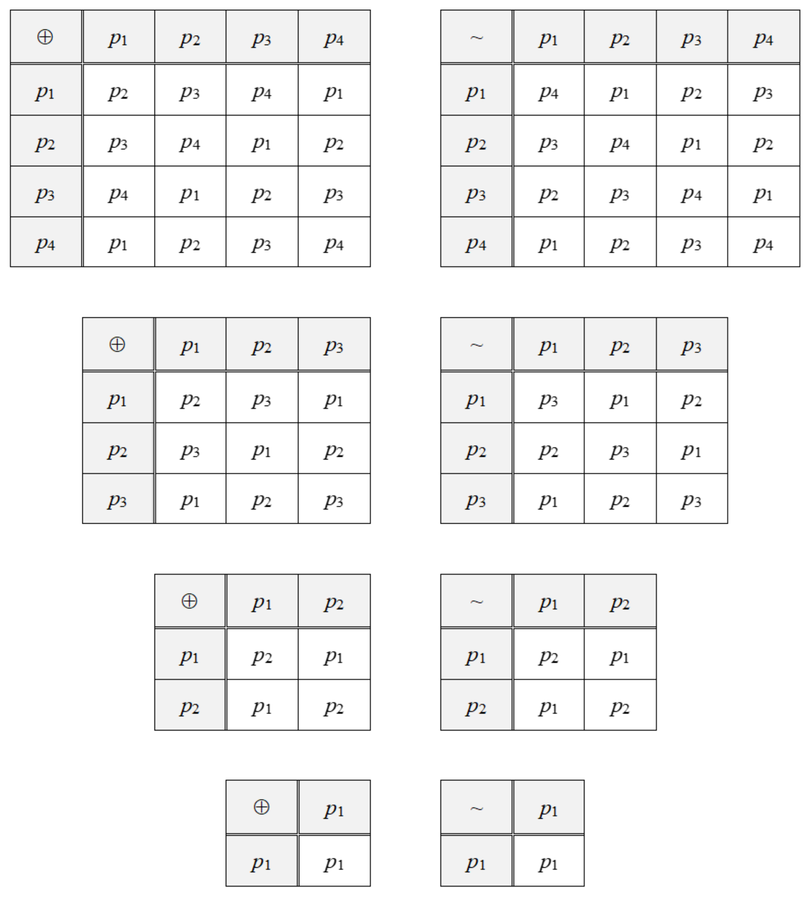Because the acceleration factors c₁^extern, c₂^extern, c₃^extern and the random redirecting factors r₁^extern(t), r₂^extern(t), r₃^extern(t) are associated with external space, not to the computer space (i.e., the human mind), the multiplication operation ⊗ between a GIV and a coefficient has no sense in Equation (9). However, for addition ⊕ and subtraction ~of GIVs, specific rules must be defined. In this respect, the existence of a maximum of four GIVs to each performance indicator is considered for simplifying the formalism for addition ⊕ and subtraction ~of GIVs. The nonconventional addition ⊕ and subtraction ~of GIVs is happening in an abstract space, defined by a finite set of elements (1, 2, 3, or 4, by the case). The formalism is presented in Figure A1 under a matrix form, showing all four possible cases (i.e., subsets with four GIVs, subsets with three GIVs, subsets with two GIVs, and subsets with a single GIV).

In Figure A1 from Appendix A, the rule is that the GIV from the raw is added (or subtracted, by the case) with (from) the GIV from the column. Symbols p₁, p₂, p₃, p₄ in Figure 1 describe the GIVs in a subset, in the order of their ranks (that is, the GIV with the highest rank in the subset is p₁). More insights on how these operations are applied are given in the case study from Section 5. The convergence of the algorithm is verified by comparing the evolution of the utility function T (Equation (4)) from one iteration to the next one, as well as by comparing the evolution of the result of subtracting the target value and the current value for each performance indicator (see Equation (5)).

4.3. Roadmap of the SCV Algorithm

Based on the developments introduced in Section 4.2, the SCV algorithm consists of seven steps.

Step 1: Define the number of particles in the swarm and the number of iterations. Because a particle is a possible solution to the problem under consideration, a set of solutions equal to the number of particles must be proposed at each iteration. From practical considerations, this paper recommends limiting the number of particles in the swarm at s = 3. Knowing the number of possible combinations of GIVs (see Equation (6)), the maximum number of iterations is determined as N = round(H/s − 0.5).

Step 2: Feed the database with support elements. Information about the performance indicators, their related GIVs, their weights, and targets (see Equation (4)) are introduced in the system.

Step 3: Particle initialization. For each particle in the swarm, a GIV from the subset is assigned to the level of each performance indicator. A possible way to initialize this state is given in Section 4.2.2.

Step 4: Concurrent conceptualization of the first set of solutions based on the initial position of particles in the swarm. For each combination of GIVs defined at step 3 (i.e., for each initial position of the particles in the system), a solution to the problem is formulated. Thus, s initial solutions should emerge by directing the conceptualization effort towards the intervention zones recommended by the GIVs assigned at step 3. There is no barrier at this step to use any kind of supporting tool (e.g., modeling and simulation, morphological charts, mind maps, etc.) to inspire and/or guide engineers in finding solutions within the zones of interventions suggested by GIVs. Once solutions are formulated, the values for V_Ei, i = 1, ..., n are determined (see Equation (4)).

Step 5: Calculation of the utility function T concerning each particle and determining the best local solutions and the best global solution. At each iteration, for each particle, the utility function T is calculated (see Equation (4)). Results are compared with the target value, which is 1 (∆T = 1 − T; ∆T → 0). A set of s values for ∆T will result (one for each particle in the system). The solution with the smallest ∆T is chosen as the best solution in the swarm (z_t in Equation (9)). For the positions y_1,1, ..., y_s,1 (y_i,t, i = 1, ..., s; t = 1) in Equation (9), afferent to the first iteration, initialization will be done according to the recommendations from step 3. For the next iterations, ∆T belonging to all solutions to the level of each particle and to the global level will be compared each other, and the z_t and y_i,t, i = 1, ..., s will be selected for which ∆T is the smallest at global level and local levels, respectively. Practically, as iterations progress, the number of solutions increases. At iteration t, s × t solutions are compared for selecting z_t, and t solutions are compared for selecting the best local solution for each particle.

Step 6: Algorithm indexing and calculation of new positions and velocities for particles. Equations (8) and (9) are used for starting a new iteration. Position u is randomly selected from all solutions proposed up to that moment in the previous iterations. Practically, a solution is identified within the algorithm using a combination of GIVs. Therefore, an association between every solution and a well-defined combination of GIVs is realized. A modality to do this is by identifying the particle and the iteration. For example, for particle 2, at iteration 5, the solution could be symbolized as SOL (2:5).

Step 7: Convergence and termination condition verification. Equation (5) is considered at this step. Until the number of iterations t respects the condition t < N, the algorithm is resumed from step 4.

5. Illustrative Example

The SCV algorithm is further exemplified for designing the structure of a reconfigurable machine tool with adjustable functionality [67,68,69]. Reconfigurable machine tools are manufacturing equipment whose structure can be modified in a way they are capable of providing alternative functionality and/or capacity, as it is required at a certain moment by production (no more, no less) [66]. They are designed around common characteristics of a family of parts [67]. By embedding this property, a reconfigurable machine tool fits the paradigm of industry 4.0 because it facilitates rapid adaptability and agility with minimum waste (i.e., underutilized production resources) and fits the paradigm of the circular economy. It is aligned with value optimization, stewardship, system thinking, and the 6R eco-innovation principle [6].

5.1. Problem Definition

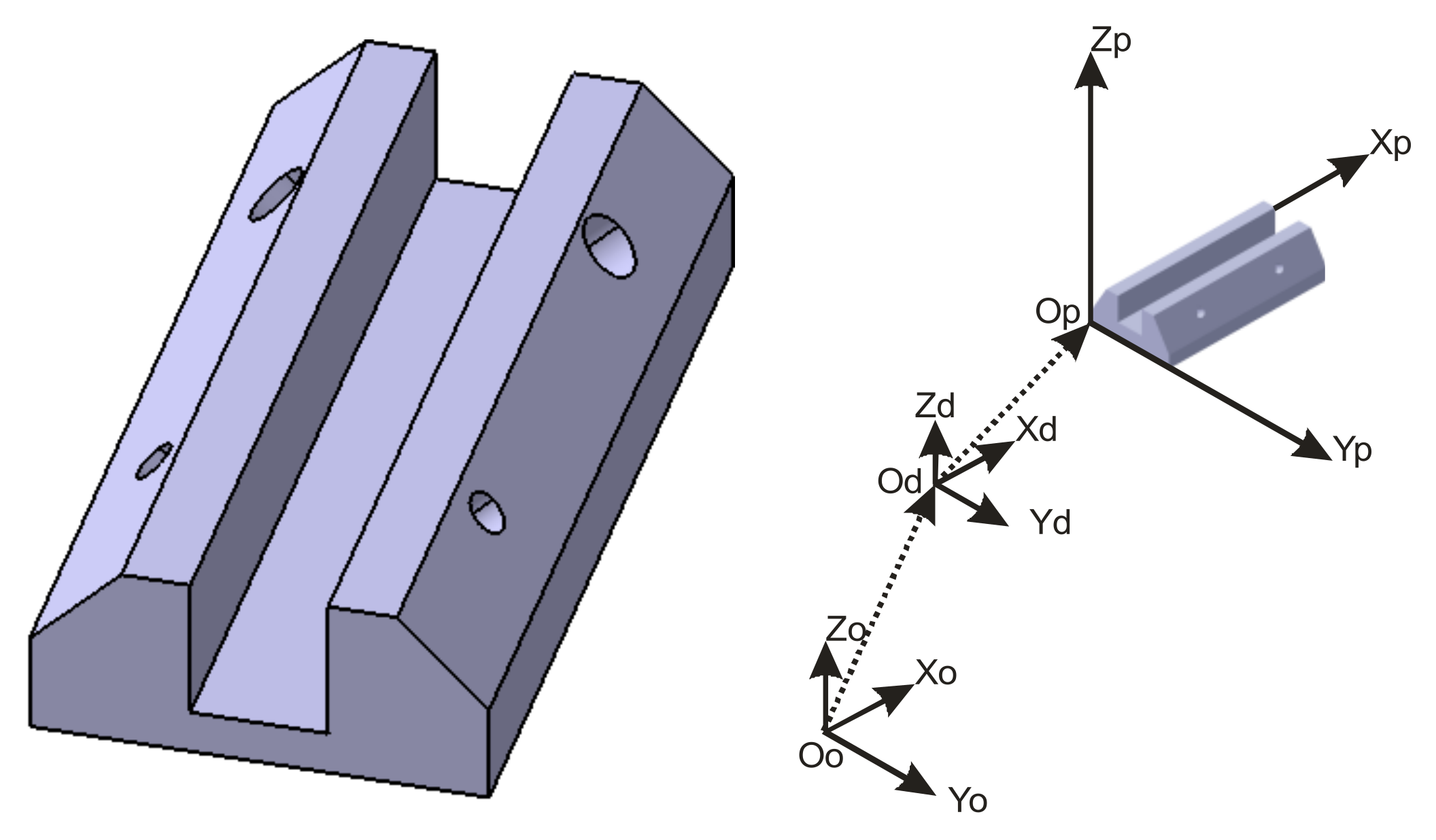
Figure 1 shows the generic part associated with the reconfigurable machine tool whose configuration must be designed in this case study, as well as its reference system. Thus, OpXpYpZp is the part (piece) reference system, OdXdYdZd is the reference system of the part-gripping device, OoXoYoZo is the reference system of the machine tool, OdOp is the vector of transformation from OdXdYdZd to OpXpYpZp, OoOd is the vector of transformation from OoXoYoZo to OdXdYdZd (Figure 1).

Figure 2 highlights the sequences of manufacturing part surfaces. TH_x indicates the technological translation motion along axis x, TH_y the technological translation motion along axis y, TH_z the technological translation motion along axis z, with RH_x the technological rotation motion around axis x, RH_y the technological rotation motion around axis y, and RH_z the technological rotation motion around axis z.

The translation motion for tool positioning along axis x is denoted with TP_x, with TP_y the translation motion for tool positioning along axis y, TP_z the translation motion for tool positioning along axis z, RP_x the rotation motion for tool orientation around axis x, RP_y the rotation motion for tool orientation around axis y, and RP_z the rotation motion for tool orientation around axis z. Considering an axis A: as a result of tool orientation because of two or more rotary motions RP_x, RP_y, RP_z, the axis is denoted with TH_A, the translation motion of the tool along with axis A, and with RH_A the rotation motion of the tool around axis A.

Using the notations above, the following motions are necessary to manufacture the five surfaces of the generic part (see in Figure 1, from # 2 to #6):

• Surface 1 (#2 in Figure 2): TP_x, TP_y, TP_z, RP_x, TH_x, RH_A;
• Surface 2 (#3 in Figure 2): TP_x, TP_y, TP_z, RP_x, RP_z, TH_x, RH_A;
• Surface 3 (#4 in Figure 2): TP_x, TP_y, TP_z, TH_x, RH_z;
• Surface 4 (#5 in Figure 2): TP_x, TP_y, TP_z, RP_x, TH_A, RH_A;
• Surface 5 (#6 in Figure 2): TP_x, TP_y, TP_z, RP_x, RP_z, TH_A, RH_A.

It is important to highlight here that both the posing motions and technological motions of the reconfigurable machine tool can be obtained from various structural combinations. The goal is to identify those structural combinations, which maximize the utility function T (Equation (4)).

5.2. Design Planning

For conceptualizing the reconfigurable machine tool, in this case, study, we selected a set of E-KPIs that come in front of the paradigms of industry 4.0 and circular economy. At this point, we want to highlight the fact that selecting the E-KPIs for this case study was influenced by the concept of “waste” applied in lean manufacturing; that is, to eliminate all activities that do not bring value-added to the system. In an eco-smart manufacturing system from the paradigm of industry 5.0, modules of machines come as independent cyber-physical systems, with plug-and-play capabilities, in a master-slave reconfigurable architecture. This type of solution has already been investigated by the authors of this paper and is published in [10]. Thus, in the design problem under investigation in this case study, we consider all modules embedding this capacity, which, in principle, is a key KPI of reconfigurability but not a dependent one from other KPIs. Therefore, it is not included in the optimization problem from this research.

Considering the aspects mentioned above, we finally limited the optimization problem to five performance indicators (E-KPIs) for the conceptual design of the reconfigurable machine tool with adjustable functionality under the space of possibilities imposed by the family of parts described by the generic part from Figure 1:

• Time for reconfiguring machine’s functionality (code in the set: 1 (i = 1); trend: minimize (k(1) = −1));
• Variety of available constructive modules of the machine (code in the set: 2 (i = 2); trend: maximize (k(2) = 1));
• Number of locations for the interfaces between modules (code in the set: 3 (i = 3); trend: maximize (k(3) = 1));
• Number of possible configurations (code in the set: 4 (i = 4); trend: maximize (k(4) = 1));
• Granularity level (code in the set: 5 (i = 5); trend: maximize (k(5) = 1)).

Based on expert judgments and applying a structured ranking tool (in this case the analytical hierarchy process [24,25]), the following normalized-to −1 value weights are assumed in this case study: β₁ = 0.11; β₂ = 0.25; β₃ = 0.26; β₄ = 0.24; β₅ = 0.14. The target values for the performance indicators in this case study are: V_T1 = 120 min; V_T2 = 10 #; V_T3 = 2 locations/module; V_T4 = 12 #; V_T5 = 75%.

To measure the effective values V_Ei, i = 1, ..., 5, while applying the SCV algorithm, the following aspects are considered:

• If a certain module in the structure is of pure rotation or translation, the assumption is that it can be easily ordered from the producer, thus available when required.
• If a certain module in the structure is of pure rotation or translation, it is assumed that it is no difficult to consider two locations on the module for joining with other modules.
• If it is denoted with g_r the granularity level of the structure, with n_f the number of functionalities of the structure, and with n_m the number of modules integrated into the structure to ensure the necessary functionalities for manufacturing the generic part, the following equation is established: g_r= (n_f /n_m)·100[%].
• If it is denoted with t_r the time required for reconfiguration, with t_m the estimated average time for assembly/disassembly of a module (e.g., approx. 20 min), with m_i the number of modules that must be replaced or repositioned, with m_a the number of new modules that must be added in the system, and with t_a the time allocated for various adjustments (e.g., here, t_a could be considered as 20% from t_m·(m_i + m_a)), the following equation is established: t_r = t_m·(m_i + m_a) + t_a.

5.3. Identification of GIVs

For each performance indicator, the set of GIVs must be determined. The conflict associated with each performance indicator is determined in the first step. Thus, the following results are obtained:

• Reconfiguration time (#1): adaptation speed versus automation level (GEP #9 versus GEP #38 in TRIZ language (see TRIZ-MC, p. 280, [32]));
• Module availability (#2): the time required for reconfiguration versus the waste of modules (GEP #9 versus GEP #23 in TRIZ language (see TRIZ-MC, p. 280, [32]));
• Number of interfaces/module (#3): convenience in use versus complexity of solution (GEP #33 versus GEP #36 in TRIZ language (see TRIZ-MC, p. 280, [32]));
• Number configurations (#4): adaptability versus waste of functional units (GEP #35 versus GEP #23 in TRIZ language (see TRIZ-MC, p. 280, [32]));
• Granularity (#5): adaptability versus complexity of control and precision (GEP #35 versus GEP #37 in TRIZ language (see TRIZ-MC, p. 280, [32])).

For the contradictions above, the GIVs revealed by TRIZ-MC [32] are put into evidence in

Table 1. GIVs for the case study under consideration.

Performance Indicator	GIV Position in TRIZ Table	GIV Description (See TRIZ Table of 40 GIVs, p. 284, [32])
#1	#10	Perform in advance arrangements of components
	#18	Use the “resonance frequency”
#2	#10	Perform in advance arrangements of components
	#13	Inversion (e.g., from mobile into immobile or vice versa)
	#28	Replace the rigid system with a flexible one
	#38	Strong interactions (e.g., enrich the system with elements)
#3	#12	Ensure equipotentiality
	#17	Multilayer assembly and multidimensional motions
	#26	Use simple copies instead of a compact, complex system
	#32	Use some additive elements
#4	#2	Extract the disturbing part from the system
	#10	Perform in advance arrangements of components
	#13	Inversion (e.g., from mobile into immobile or vice versa)
	#15	Create interchangeable modules with automatic adjustment
#5	#1	Increase the level of segmentation

.

GIV #10 occurs three times in Table 1. Considering the value weights of the associated performance indicators, β₁ = 0.11, β₂ = 0.25 and β₄ = 0.24, the rank of GIV #10 is b(#10 )= 0.60. Similarly, with the logic above, the ranks of the other GIVs from Table 1 are determined. They are b(#18) = 0.11, b(#13) = 0.49, b(#28) = 0.25, b(#38) = 0.25, b(#12) = 0.26, b(#17) = 0.26, b(#26) = 0.26, b(#32) = 0.26, b(#2) = 0.24, b(#15) = 0.24, b(#1) = 0.14.

Thus, GIVs in the subset belonging to each performance indicator can be ordered, starting with the highest rank. In cases where the ranks of two GIVs in the subset are of the same value, the position of GIVs in the subset is given randomly. For example, all GIVs belonging to performance indicator #3 in Table 1 have the same rank. Thus their order in the subset may be {#26, #32, #12, #17}. Based on the calculated ranks, the result of ordering GIVs is illustrated in

Table 2. Order of GIVs.

Performance Indicator	Position 1		Position 2		Position 3		Position 4
	GIV	Symbol	GIV	Symbol	GIV	Symbol	GIV	Symbol
#1	#10	p1	#18	p2
#2	#10	p1	#13	p2	#28	p3	#38	p4
#3	#26	p1	#32	p2	#12	p3	#17	p4
#4	#10	p1	#13	p2	#15	p3	#2	p4
#5	#1	p1

. Symbols associated with GIVs in Table 2 are taken from Figure A1.

Addition ⊕ and subtraction~ in Equations (8) and (9) using the symbols from Table 2 are further exemplified. In this respect, it is assumed for example, that particle #1 in the swarm at iteration t is defined by the following GIVs of the performance indicators: performance indicator #1 by GIV #10, performance indicator #2 by GIV #28, performance indicator #3 by GIV #17, performance indicator #4 by GIV #2, performance indicator #5 by GIV #1. Using symbols from Equation (8) this combination is represented as 1₁{j₁(t)}, 2₁{j₂(t)}, 3₁{j₃(t)}, 4₁{j₄(t)}, 5₁{j₅(t)} and using symbols from Figure A1 it looks like 1₁{p₁}, 2₁{p₃}, 3₁{p₄}, 4₁{p₄}, 5₁{p₁}. Thus, the position of particle #1 at iteration t can be expressed using the symbols in Equation (8) and Figure A1 as x₁(t) ={1₁{p₁}, 2₁{p₃}, 3₁{p₄}, 4₁{p₄}, 5₁{p₁}}^T. It is assumed that at iteration t + 1, after applying Equation (9), particle #1 has the velocity v₁(t + 1) = {v₁{p₁}, v₁{p₁}, v₁{p₂}, v₁{p₃}, v₁{p₄}}^T. Using the formalism from Figure A1, the sum x₁(t) ⊕ v₁(t + 1) leads to a new position of particle #1, corresponding to iteration t + 1, x₁(t + 1) = {1₁{p₁⊕p₁}, 2₁{p₃⊕p₁}, 3₁{p₄⊕p₂}, 4₁{p₄⊕p₃}, 5₁{p₁⊕p₄}}^T or x₁(t + 1) = {1₁{p₂}, 2₁{p₄}, 3₁{p₂}, 4₁{p₃}, 5₁{p₁}}^T. Translating this result in the space of GIVs, the position x₁(t + 1) of particle #1 at iteration t + 1 is given by GIV #18 for the performance indicator #1, GIV #38 for the performance indicator #2, GIV #32 for the performance indicator #3, GIV #15 for the performance indicator #4, and GIV #1 for the performance indicator #5 (see notations from Table 2). Subtraction is done on the same logic, but matrices from Figure A1 associated with this operation are considered. For example, it is assumed that u_t is the position of particle #2 at iteration t − 5. In addition, it is assumed that x₂(t − 5) = {1₂{p₂}, 2₂{p₂}, 3₂{j₃(p₃}, 4₂{p₂}, 5₂{p₁}}^T. The subtraction u_t ~x₁(t) becomes x₂(t − 5) ~x₁(t) = {1₂{p₂~p₁}, 2₂{p₂~p₃}, 3₂{p₃~p₄}, 4₂{p₂~p₄}, 5₂{p₁~p₁}}^T or u_t ~x₁(t) = {1₁{p₁}, 2₁{p₁}, 3₁{p₁}, 4₁{p₂}, 5₁{p₁}}^T. In the space of GIVs this result is j₁(t) ≡ GIV # 10, j₂(t) ≡ GIV #10, j₃(t) ≡ GIV #26, j₄(t) ≡ GIV #13, j₅(t) ≡ GIV #1.

5.4. Algorithm Initialization

For defining the combination of GIVs for algorithm initialization, recommendations from Section 4.2.2 are considered. For s =3 particles in this case study, the following situation is considered:

• Particle #1: indicator #1{GIV #10}, indicator #2 {GIV #10}, indicator #3 {GIV #26}, indicator #4 {GIV #10}, indicator #5 {GIV #1},
• Particle #2: indicator #1{GIV #10}, indicator #2 {GIV #13}, indicator #3 {GIV #26}, indicator #4 {GIV #10}, indicator #5 {GIV #1},
• Particle #3: indicator #1{GIV #10}, indicator #2 {GIV #28}, indicator #3 {GIV #26}, indicator #4 {GIV #10}, indicator #5 {GIV #1}.

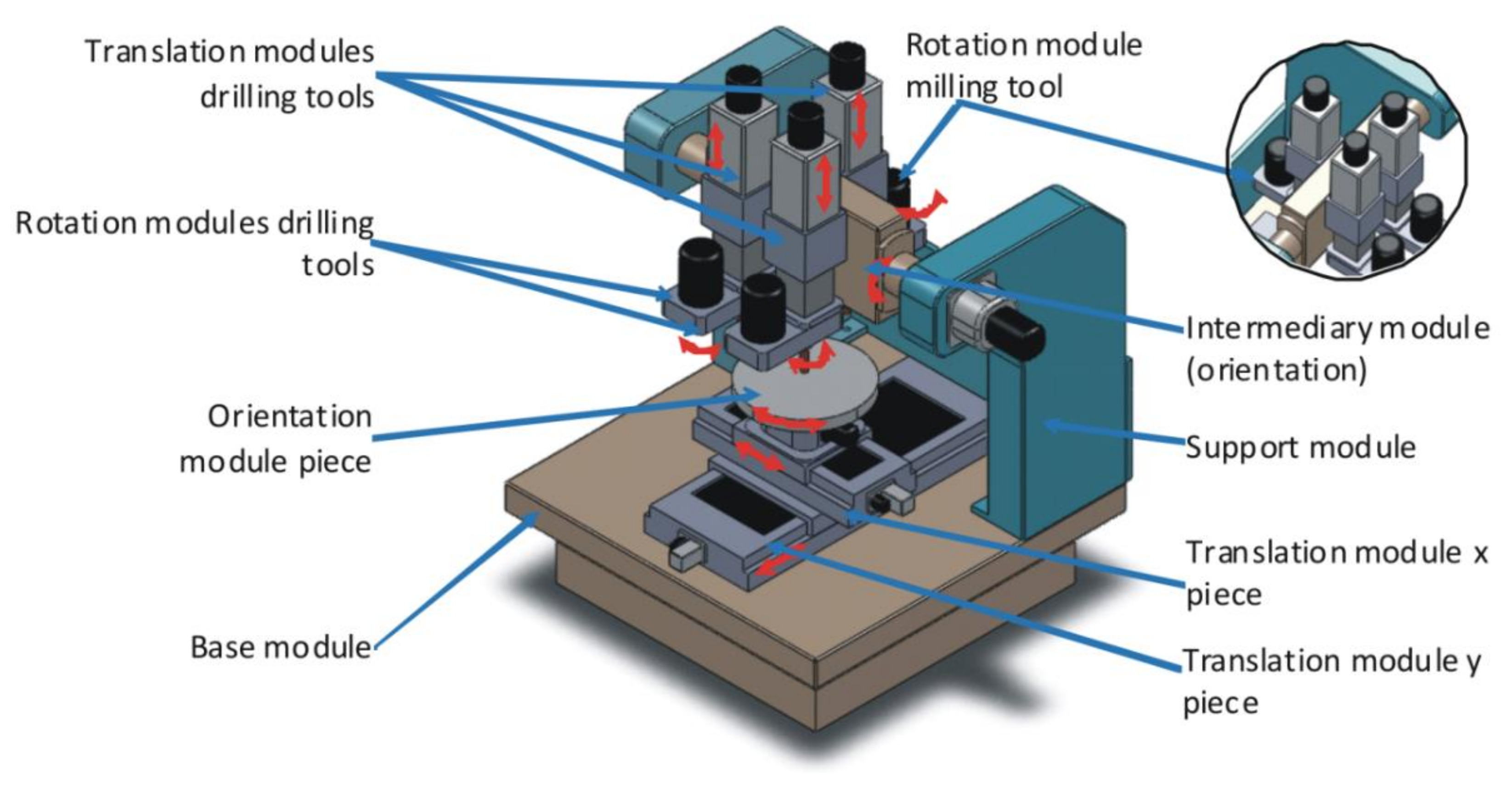
Symbolically, the initialization condition looks like: 11{p1}, 21{p1}, 31{p1}, 41{p1}, 51{p1}; 12{p1}, 22{p2}, 32{p1}, 42{p1}, 52{p1}; 13{p1}, 23{p3}, 33{p1}, 43{p1}, 53{p1}. In a practical language, the following directions (see Table 1) are given for conceptualizing the first three possible variants of the reconfigurable machine tool under consideration:

• Variant 1 should be defined by the combination: reduce the time for reconfiguration by “arranging in advance some functional units” AND increase variety of available modules by “arranging in advance some functional units” AND ensure sufficient interfaces by “using simple copies instead of a complex system” AND increase the number of possible configurations by “arranging in advance some functional units” AND reach the granularity level by “increasing the level of segmentation”;
• Variant 2 should be defined by the combination: reduce the time for reconfiguration by “arranging in advance some functional units” AND increase variety of available modules by “inversion: from mobile to immobile or vice versa” AND ensure sufficient interfaces by “using simple copies instead of a complex system” AND increase the number of possible configurations by “arranging in advance some functional units” AND reach the granularity level by “increasing the level of segmentation”;
• Variant 3 should be defined by the combination: reduce the time for reconfiguration by “arranging in advance some functional units” AND increase variety of available modules by “replacing the rigid system with a flexible one or with a field” AND ensure sufficient interfaces by “using simple copies instead of a complex system” AND increase the number of possible configurations by “arranging in advance some functional units” AND reach the granularity level by “increasing the level of segmentation”.

The three possible solutions that will emerge from applying the guidelines above represent the initialization particles of the SCV algorithm. Based on these guidelines and using the expertise and creative potential of the team involved, the first three possible variants are illustrated in Figure 3, Figure 4 and Figure 5.

For variant 1 in Figure 3, GIVs are identified as follows: increase the level of segmentation is reflected in a higher number of functional modules, arrangement in advance of some functional units is reflected in the concept of the positioning structure of the tools, simple copies instead of a complex system is found in the idea of using some similar (independent) units for driving and positioning each tool. Granularity for variant 1 is g_r= 45% (n_f = 5, n_m = 11; see Section 5.2). The estimated time for structure reconfiguration in the case of variant 1 is t_r = 264 min (t_m = 20 min in this case study, m_i = 4, m_a = 7; see Section 5.2). For calculating t_r in the case of variant 1, the following operations for structure reconfiguration were considered: the supporting columns and two modules for drilling operation are replaced, two modules for milling operations are repositioned, as well as four modules for drilling operations, an orientation module, a supporting structure and a module for piece orientation are added in the system. Reconfiguration is considered for the worst-case scenario (from the simplest piece to the most complex piece in the family of pieces).

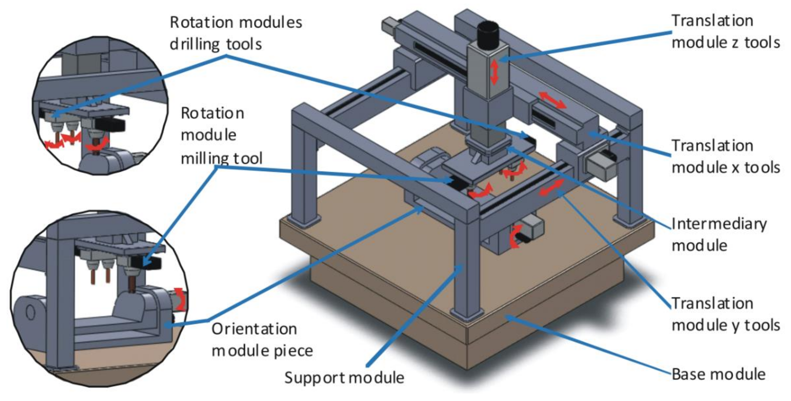
For variant 2 (see Figure 4), GIVs related to segmentation, simple copies and arrangement in advance are similarly exploited as in the case of variant 1 but reflected in a different concept (a gantry structure). The inversion principle is identified in reducing the degrees of freedom of the supporting platform for the working piece. For this variant, granularity is gr= 63% (nf = 5, nm = 8), and the reconfiguration time is tr = 192 min (tm = 20 min, mi = 2, ma = 4). In the case of variant 2, reconfiguration requires the replacement of a drilling module, repositioning of the milling module, the addition of a piece orientation module, two drilling modules and a horizontal translation module.

In the case of variant 3 (see Figure 5), GIVs related to segmentation, simple copies and arrangement in advance are similarly exploited as in the case of variant 1 but reflected in a different concept. The GIV requiring replacement of a rigid system with a more flexible one is introduced in variant 3 in the increase of the degrees of freedom of the supporting platform for the working piece and the solution of posing the working tools. For this variant, granularity is g_r= 63% (n_f = 5, n_m = 8), as in the case of variant 2, and the reconfiguration time is t_r = 72 min (t_m = 20 min, m_i = 0, m_a = 3). In the case of variant 3, reconfiguration requires the addition of two modules for drilling, a module for piece orientation and removal of two modules (piece orientation and drilling). Here, the reconfiguration time t_r exceeds the target (120 min).

The SCV algorithm considers the target as being also the effective value introduced in Equation (4) for calculating the utility function T. A software application written in Java was developed to calculate the utility function T from Equation (4) and the convergence index from Equation (5) for each particle, as well as for performing all operations from Equations (8) and (9). For example, a screenshot from this application highlighting the results after four iterations of the SCV algorithm is shown in Figure 12. Making the calculations (see Equation (4)), at iteration 1 the utility function T for particle 1 is T₁ = 0.88, for particle 2 is T₂ = 0.94, and for particle 3 is T₃ = 0.98. Thus, the maximum value after iteration 1 is attained by particle 3. The convergence index, in this case, is 0.02 (Equation (5)).

5.5. Solution Improvement by Incrementing the SCV Algorithm

For the second iteration, the combination of GIVs given by the SCV algorithm is: 1₁{p₂}, 2₁{p₄}, 3₁{p₂}, 4₁{p₁}, 5₁{p₁}; 1₂{p₂}, 2₂{p₃}, 3₂{p₂}, 4₂{p₂}, 5₂{p₁}; 1₃{p₂}, 2₃{p₂}, 3₃{p₂}, 4₃{p₂}, 5₃{p₁}. These results are obtained by applying the formalism from Equations (8) and (9). Table 2 shows the associated GIVs for the symbols p₁, p_2, p_3, p₄ above. For particle 1, the proposed variant is shown in Figure 6. In this case granularity is g_r= 83% (n_f = 5, n_m = 6), and the reconfiguration time is t_r = 24 min (t_m = 20 min, m_i = 1, m_a = 0). The utility function in this case is T₁ = 1, thus variant 4 in Figure 6 might be considered one of the reliable solutions for the machine tool.

For particle 2, at iteration 2, the solution is shown in Figure 7. For variant 5 the following results are obtained: granularity g_r= 83% (n_f = 5, n_m = 6), and the reconfiguration time is t_r = 24 min (t_m = 20 min, m_i = 1, m_a = 0). The utility function in this case is T₂ = 1, thus variant 5 in Figure 8 may be considered another reliable solution for the machine tool.

For particle 3, the solution from Figure 8 is proposed after the second iteration. In this case, granularity is g_r= 71% (n_f = 5, n_m = 7), and the reconfiguration time is t_r = 24 min (t_m = 20 min, m_i = 1, m_a = 0). The utility function in this case is T₃ = 0.99.

One can conclude that after the second iteration of the SCV algorithm, at least two reliable solutions were identified (variant 4 and variant 5, both reaching the target of the utility function and leading to a convergence index equal to 0). The best position in the swarm after the first and second iterations is reached by particle 1 (variant 4:1₁{p₂}, 2₁{p₄}, 3₁{p₂}, 4₁{p₁}, 5₁{p₁}).

In principle, the SCV algorithm could be stopped after the second iteration. However, continuation with one or two more increments may be useful to see if there is some more potential for innovation (e.g., in this case, particle 3 still has further potential to explore the space of solutions). If the new iterations lead to distancing from the targets for the utility function and the convergence index, algorithm incrementing should be stopped.

Thus, the third iteration of the SCV algorithm leads to the following combination of GIVs: 1₁{p₁}, 2₁{p₃}, 3₁{p₁}, 4₁{p₁}, 5₁{p₁}; 1₂{p₁}, 2₂{p₂}, 3₂{p₁}, 4₂{p₁}, 5₂{p₁}; 1₃{p₁}, 2₃{p₁}, 3₃{p₁}, 4₃{p₁}, 5₃{p₁}. Vectors’ significance is given in Table 2, with further details in Table 1. The new positions of particles in the swarm are identical with the positions from iteration 1, excepting the fact that particle 1 takes the place of particle 3 and vice versa. Therefore, at the third iterations, particles move away from the maximum position in the searching space. Thus, a new iteration is considered.

At the fourth iteration, the space for solution search is given by the following combination of GIVs: 1₁{p₁}, 2₁{p₃}, 3₁{p₃}, 4₁{p₃}, 5₁{p₁}; 1₂{p₁}, 2₂{p₄}, 3₂{p₃}, 4₂{p₃}, 5₂{p₁}; 1₃{p₁}, 2₃{p₁}, 3₃{p₃}, 4₃{p₃}, 5₃{p₁}. Vectors’ significance is given in Table 2, with supplementary details in Table 1. Figure 10 displays the solution associated with particle 1 at iteration 4 of the SCV algorithm. In this case, granularity is g_r= 83% (n_f = 5, n_m = 6), the reconfiguration time is t_r = 24 min (t_m = 20 min, m_i = 1, m_a = 0). The utility function is T₁ = 1 and the convergence is 0. Thus, variant 7 from Figure 9 is another reliable solution for the structure of the machine tool.

Figure 10 illustrates the solution of particle 2, at iteration 4. For variant 8, the following results are revealed: granularity g_r= 71% (n_f = 5, n_m = 7), reconfiguration time t_r = 24 min (t_m = 20 min, m_i = 1, m_a = 0). The utility function is T₂ = 0.99.

For particle 3, at iteration 4 of the SCV algorithm, the result is shown in Figure 11. Solution in this case reveals a granularity g_r= 71% (n_f = 5, n_m = 7), a reconfiguration time t_r = 24 min (t_m = 20 min, m_i = 1, m_a = 0). The utility function in this case is T₃ = 0.99. Thus, the best position at iteration 4 is given by the first particle in the swarm.

In conclusion, after four iterations, three reliable solutions were identified for the machine tool (variants 4 and 5 from iteration 2 and variant 7 from iteration 4). For this example, iterations are stopped at this point.

Figure 12 illustrates the implementation of the SCV algorithm in a dedicated software application written in Java. The left-side window shows the results after the second iteration, whereas the right-side window shows the results after the fourth increment.

As Figure 12 shows, in all cases where the current value exceeds the target of a certain parameter, the value of the target is introduced for calculating the utility function. This is appropriate for the intended objective, and it is done in this way to follow the form imposed by the utility function in Equation (4). Another important remark is about the values given to three performance indicators (i.e., variety of available modules, number of locations for interfaces, number of possible configurations) in all the variants highlighted in this example. It is seen in Figure 12 that, for all cases, these three performance indicators reached their target values. The reason is further justified.

For module availability, all modules are simple rotation or translation units; thus, they can be easily ordered. Because all modules are of pure rotation or translation, there is no difficulty in that each module is designed with two locations for interfacing with other modules. If all parts in the family of parts (see Figure 1 for the generic part) can be manufactured with any of the proposed variants, configurability reaches the target in all cases.

6. Discussion on the Results from the Case Study

Results from Section 5 reveal that more solutions can be defined for maximizing the utility function of a certain multicriteria-related design problem. From this perspective, the selection of the final solution requires supplementary criteria for analysis, criteria that are not necessarily related to the design process. For example, referring to the case study illustrated in this paper, an important selection step involves identifying suppliers for the functional modules identified to the three candidate variants of the machine tool. This process could lead to several cases. One such case is when one or two of the three solutions are rejected because no suppliers exist for some of their functional units. Another case is when all three solutions are rejected because of a lack of suppliers for some functional modules. In this situation, another variant in the set must be selected (one, which is close as global performance to the three variants, but, which can be provided by suppliers of modules, e.g., variants 6, 8 or 9), or the SCV algorithm is further applied for defining a new solution. If all three or at least two of the preferable variants (4, 5 and 7) can be supplied, supplementary analyses are considered, too. In this respect, static and dynamic analyses, including thermal behavior and/or other behavioral analyses, are performed for each variant (e.g., using 3D finite element formalisms). If the technical analyses still do not reveal a final solution, the economic criterion should be further considered (e.g., servitization-led business models based on subscription). If the economic criterion leads to slight differences between variants, the business risk is added to the analysis. This could involve issues about guarantees from suppliers, response time, etc.

7. Discussion on Reconfigurable Machine-Tool Design

In the context of industry 5.0, reconfigurable machine tools play a crucial role. They facilitate agility in production and cost-effectiveness along the lifecycle. Today, technologies allow designing functional modules of machine tools that can be interconnected via distributed control architectures that facilitate convertibility and scalability. Thus, from a technological point of view, engineering achieved the level of development that allows the design of reconfigurable systems. However, reconfigurable machine tools are still rarely seen in the industry. This is a consequence of the fact that manufacturing organizations are still lagging in adopting circular economy and lifecycle models, and their markets did not reach yet the stage where mass customization is critical. However, signs indicate that this is the trend, and producers must be prepared for that moment.

In this foreseen paradigm, the conceptualization of reconfigurable machine tools remains a challenge because tools must be designed in context. This requires a good understanding of the families of parts to be manufactured over longer periods, in terms of financial sustainability (e.g., net present value and return on investment), ecological sustainability (e.g., longer use of functional modules, more reconditioning and reuse of such modules and less material disposal), and social sustainability (e.g., support of mass customization with fewer resources, assurance of coexistence of machines and people in the factory shop, etc.). Hence, reconfigurability is more than the capacity to interconnect functional modules in different machine tool architectures. It is also about finding the best architectures for each manufacturing context (minimum number of modules and the most appropriate types of modules that can be configured and reconfigured over the lifecycle of a family of products to meet all manufacturing needs as required without involving redundant or underutilized units). For this challenge, this paper introduces a design algorithm that helps engineers to narrow the space of investigation, speed up the time, and reduce the effort involved for reconfigurability optimization in machine-tool design.

8. Conclusions

The conceptual design of complex products is an iterative process involving many factors of influence and plenty of options in the search for solutions. Reducing the number of attempts until a reliable solution is defined represents an important goal in this process. Therefore, the focalization of the conceptualization effort towards the key issues of the problem is desirable. In this respect, a boundary of the design space is defined using performance criteria and related targets. This space of constraints creates premises for exploiting creativity.

This paper concentrates on combining optimal design philosophy with structured management of creativity for reducing the number of iterations until a mature solution to a design problem is envisaged. This is possible by leading searches every time towards those directions of intervention that are significant for the design problem under consideration (i.e., framed by the laws of ideality and convergence). Optimal design algorithms are usually applied after concept creation for improving some measurable parameters of the solution. In this paper, the optimal design is applied in an earlier design phase, specifically for defining the concept. Moreover, it is known that the mathematical formalisms behind the optimal design algorithms are automatically conduced for determining the best solution in the considered space of design, with no room for human intervention during algorithm application. The formalism proposed in this paper lets engineers interfering in a structured way (via some well-defined vectors of intervention) in the evolutionary design algorithm (in all iterations) for bringing their creative potential and knowledge in solution creation. PSO combined with TRIZ-based structured innovation formalisms look to be suitable for performing this task. The case study presented in the paper is very illustrative in this respect.

The quality of the SCV algorithm is the fast convergence to a reliable solution without diminishing the creative role of engineers and without narrowing the space of search. However, instead of adopting a trial-and-error approach, which is usually the core modality of action in conceptual design, it increases the effectiveness of ideation by directing the creative and experiential capacity of engineers towards those directions that indicate the highest potential for the ideal solution. Thus, the conceptual design, which induces the highest impact on later developments, is guided by an expert system. Imagining that engineers would benefit from a large database of technical solutions, the SCV algorithm can semi-automatize the conceptual design process or even automatize it using a supervised machine-learning algorithm or a reinforcement learning algorithm. However, this requires access to a large pool of data. Even if for the problem introduced in the case study, such databases are not yet available, in several other engineering fields, this can be feasible. Therefore, we claim that the SCV algorithm can experiment in future research as part of an artificial intelligence algorithm for conceptual design. From this perspective, a comparative analysis of the SCV algorithm concerning other conceptual design algorithms introduced in Section 2 ([14,36,42,43]) could have merit. Nevertheless, there are some challenges and limitations of this algorithm. One challenge is that for any field of application, the proper set of GIVs must be extracted from TRIZ-MC. The second challenge is avoiding many calculations and learning the whole mathematical formalism behind it. It must be implemented in a piece of software program for easy adoption by engineers. It is also limited to those conceptual design problems where clear KPIs and targets can be formulated from the early stages and where an objective function can be shaped. In practice, not all design problems fit into this use case.

The SCV algorithm is not limited only to design reconfigurable machine tools. It can be adapted to more design problems. The SCV algorithm brings value-added to the conceptualization process by replacing the unstructured framework (trial-and-error approach) with a structured one by tackling the psychological inertia without removing creativity from the design process. At each step of the conceptual design process, the SCV algorithm directs the search towards effective positions in the design space. It also provides a measure of local and global effectiveness during process rolling, such as the subsequent searches to be directed only to other effective positions. The effectiveness of searching is ensured because both the PSO algorithm and the associated GIVs of the search positions simultaneously contribute to achieving this goal. All these elements create premises for reducing the number of iterations until a mature solution is generated.

The SCV algorithm is left for future work, in the sense of investigating the potential of other optimal design evolutionary formalisms and structured innovation means in framing the conceptual design process. New forms of the utility function could also be considered.

Because of its intrinsic characteristics, the SCV algorithm is suitable for the design problems related to modules or systems that fall in the paradigm of industry 4.0 or industry 5.0. Usually, the design of cyber-physical systems or green technologies is led by clear, measurable technical specifications. As the SCV algorithm operates with such kinds of inputs within the conceptual design, it can handle the process by breaking down complexity without affecting the overall focus. Therefore, we envisage the potential to use this algorithm for other specific systems, such as robot design, smart end-effector design, logistic unit design, controller design, etc. It can also be used as an algorithm in supervised machine learning for those cases that benefit from a big amount of data (e.g., classification of various ideas) or by increasing the efficiency of PSO algorithms in quantitative optimization problems, including multiobjective function optimization. These areas represent future lines of studies.