Performance Calculations of Gas Turbine Engine Components Based on Particular Instrumentation Methods

Abstract

This paper presents an analytical method to determine various main parameters or performances of engine components when those parameters cannot be directly measured and it is necessary to determine them. Additionally, some variants of instrumentation methods are presented, for example: engine inlet, compressor, turbine or jet nozzle instrumentation. The purpose of the instrumentation methods is to directly measure the possible parameters, which are then used as inputs in a model to determine other parameters or performance metrics. This model is based on gasodynamic process equations, and it is used to compute the air and gas parameters, such as enthalpy and entropy, which are described in polynomial form, thus leading to a more realistic calculation. At the end, this paper presents a practical example of instrumentation applied on a Klimov TV2-117A turboshaft, with a series of experimental results, following the engine testing on the test bench.

1. Introduction

Generally, most of the gas turbine engines that are in service, or are going to enter into service, have a standard minimal instrumentation [1,2], through which the engine can be monitored. In the case of a new engine project that has been developed in the design phase, and if an engine prototype based on the previous phases has been developed, a series of tests at any condition are required. For the first engine tests, it is necessary to have additional dedicated instrumentation ports and probes in the main engine sections. Therefore, the measurement of possible parameters which can be used to compute other main engine parameters is allowed. Furthermore, the area where the parameters are monitored during the engine tests on the test bench can be extended [3,4]. In many cases, when the engine is ready to enter into service, due to intellectual property reasons, the engine manufacturer does not equip the engine with all the instrumentation ports [5] as it was equipped in the testing phase. Some engine manufacturers keep the supplementary ports and install plugs on them, or they equip the engine with several inspection ports. This is a useful solution, from the testing and maintenance accessibility point of view, because it gives the possibility to install different instrumentation probes. The instrumentation of an engine depends on what experimentation is planned, or it depends on what type of practical research is used or involved [6]. If the engine will be involved in an experimental project, additional instrumentation will be needed. There are various situations when, technically, it is not possible to measure the diverse main parameters or engine performance directly [7], which also applies to the mass air flow, the overall pressure ratio, the compressor and turbine efficiency or the engine power and thrust. However, these main parameters can be indirectly determined by models (algorithms) that use different measured parameters. If the performance of a gas turbine engine is required, it is necessary to study the engine configuration, in order to analyze where instrumentation probes can be inserted and what type of probe is suitable to be mounted in the engine station. Therefore, the inlet and outlet of the engine components are defined. The level of engine instrumentation is determined in accordance with the test results, parameters that are requested and the level of experimentation. The instrumentation level is furthermore correlated with the engine components’ accessibility which allows for the instrumentation probes to be mounted.

In the case of our application, the instrumentation was divided for the gas turbine engine components, based on the availability of ports and the necessary measure points for the algorithm. For a particular industrial application, similar to our application, it is aimed for every engine component to display multiple parameters in every engine sector. The purpose of our study is to determine these parameters, and to decrease the errors in the calculation method.

Generally, in gasodynamic calculation theory, constant values of entropy and enthalpy are used in order to create an easier algorithm. In reality, the entropy and enthalpy are functions of temperature. Each method can be used in the application, but the method where the entropy and enthalpy depend on the temperature offers a higher precision. Each case has advantages and disadvantages regarding the number of instrumentation parameters. This means that the temperature-dependent enthalpy and entropy require a higher number of instrumentation parameters in determining the general engine performance or key parameters.

The method will be used for a specific case (such as an industrial application) that includes used engines that are at the end of their lifespan, not for a newly designed engine.

2. Instrumentation Methods

In this chapter, different instrumentation methods for engine components are presented, which are useful for determining some of the main parameters that cannot be measured directly and which are required for a more in-depth study [8].

The instrumentation project starts from what main parameters or performances are requested to be determined. Then, according to the type of parameters or performances required by the mathematical definition and equations, the parameters of interest are studied. In the next step, a technical study is conducted to analyze the available instrumentation ports on the engine. An analysis is also performed to determine if the available ports on the engine can be adapted as needed. As a result, the parameters that can be measured are established.

2.1. Engine Inlet Instrumentation

The engine inlet (bellmouth) is instrumented to measure the engine air flow. The mass air flow ($M_{af}$) is defined as the multiplication of density (${\rho }_s$), velocity ($V$) and cross-section ($A$) [9], where the density and velocity are functions which depend on multiple variables, such as: temperature, pressure and the Mach number.

$$M_{af}={\rho }_s(p,T)\cdot V(M,T)\cdot A;\hspace{1em}{M}_{af}=\frac{p_s}{R_a\cdot T_s}\cdot \frac{M}{\sqrt{k\cdot R_a\cdot T_s}}\cdot A$$

(1)

According to the density (${\rho }_s$) and velocity ($V$) mathematical definitions [9], the parameters that are possible to be measured are established, which are used in the density and velocity computation. One method, as presented in Figure 1a, is to instrument the bellmouth only for static pressure measurement ($p_s$), in order to measure the differential pressure ($DP$), to use the test cell air pressure ($p_0$), in order to determine the air velocity ($V$), and then to measure the test cell air temperature ($T_0$) which is used to determine the air density (${\rho }_s$). The cross-section ($A$) is determined using the bellmouth diameter ($D$).

Another method, which is more accurate, as presented in Figure 1b, is to instrument the bellmouth for static pressure measurement ($p_s$), for total pressure ($p_t$) and total temperature measurement ($T_t$), with approximately the same cross-section.

The method presented in Figure 1a requires fewer parameters on the inlet and, based on the approximation of the pressure loss coefficient on the bellmouth, it results in a higher error. The method presented in Figure 1b uses the measured parameters directly and eliminates the error that is introduced by the approximation of the pressure loss coefficients, and, as a result, it has a lower error. It is to be mentioned that any method presents an error of measurement that is introduced by the instrumentation probes.

2.2. Compressor Instrumentation

The compressor is instrumented to determine the total adiabatic efficiency and, by default, the total overall pressure ratio. The total overall pressure ratio [9] is defined as the ratio between the outlet total pressure ($p_{2.t}$) and inlet total pressure ($p_{1.t}$).

The first method, presented in Figure 2a, through which the total overall pressure ratio can be determined, is to measure only the outlet total pressure ($p_{2.t}$) because the inlet total pressure ($p_{1.t}$) can be determined from the cell air pressure ($p_0$). Compressor total adiabatic efficiency [9] is the ratio between the total specific ideal work ($l_{C.t.id}$) and the total specific actual work ($l_{C.t}$). The total specific actual work [9] ($l_{C.t}$) is the difference between the outlet total specific enthalpy ($h_{2.t}$) and the inlet total specific enthalpy ($h_{1.t}$).

$${\eta }_{C.t}=l_{C.t.id}/l_{C.t}=\left(h_{2.t.id}\left(T\right)-h_{1.t}\left(T\right)\right)/\left(h_{2.t}\left(T\right)-h_{1.t}\left(T\right)\right)$$

(2)

In this case, in order to determine the total adiabatic efficiency, only the outlet total temperature ($T_{2.t}$) must be determined because the inlet total temperature ($T_{1.t}$) is similar to the cell air temperature.

The second method, as shown in Figure 2b, shows that because of how the engine is constructed, there are situations when it is not allowed to install an outlet total pressure probe ($p_{2.t}$). In this case, it is mandatory to install an outlet static pressure probe ($p_{2.S}$) and it is necessary to know the cross-section ($A_2$) where it will be installed.

2.3. Turbine Instrumentation

The turbine is instrumented to determine the total adiabatic efficiency, the total degree of expansion or a certain inlet or outlet turbine temperature, depending on the type of test requested. Turbine total adiabatic efficiency [9] is the ratio between the total specific actual work ($l_{T.t}$) and the total specific ideal work ($l_{T.t.id}$). The total specific actual work [9] ($l_{T.t}$) is the difference between the inlet total specific enthalpy ($h_{3.t}$) and the outlet total specific enthalpy ($h_{4.t}$).

$${\eta }_{T.t}=l_{T.t}/l_{T.t.id}=\left(h_{3.t}\left(T\right)-h_{4.t}\left(T\right)\right)/\left(h_{3.t}\left(T\right)-h_{4.t.id}\left(T\right)\right)$$

(3)

According to the engine instrumentation, in the vicinity of the turbine gas temperature probe location, an accessible instrumentation method, as presented in Figure 3, is used to determine the total adiabatic efficiency. The outlet total pressure ($p_{4.t}$) must be measured, and it is also necessary to measure the total outlet temperature ($T_{4.t}$), since the total inlet temperature ($T_{3.t}$) can be determined from the energy equation applied on the combustion chamber. This happens if the total inlet temperature ($T_{3.t}$) is not measured.

The method presented in Figure 3a requires only the total outlet turbine pressure and temperature parameters, and it is not necessary to know the outlet turbine cross-section in the calculation algorithm. The method presented in Figure 3b requires for the static outlet turbine pressure to be measured. It is mandatory to know the outlet turbine cross-section, used in the calculation algorithm.

2.4. Jet Nozzle Instrumentation

In most cases, the jet nozzle is instrumented to determine the engine thrust or the outlet nozzle velocity. On the ground, on the test bench, at sea level conditions, the thrust ($F$) [9] is defined as the sum between the product of gas flow ($G_f$) and the outlet velocity ($C_5$) and the product of the outlet cross-section ($A_5$) and the differential pressure ($p_{5.t}-p_0$).

$$F=G_f·C_5+C_5·\left(p_{5.S}-p_0\right)$$

(4)

For thrust calculation, it is necessary to know the gas flow ($G_f$) and to determine the outlet velocity ($C_5$). The gas flow ($G_f$) is determined by measuring the fuel flow ($F_f$) and the air mass flow ($M_{af}$). A simple instrumentation method, as presented in Figure 4, to determine the outlet velocity ($C_5$) is indicated to measure the outlet total temperature ($T_{5.t}$) and is necessary to measure the static and total outlet pressures ($p_{5.s}$, $p_{5.t}$).

The accuracy of the measurement is given by the number of instrumentation parameters. In our case, due to the limited capacity of the ports that can be installed on the TV2-117A engine target, only one point was measured, which leads to a lower precision or a higher measurement error in the targeted section. In other cases, where the engine allows a higher number of instrumentation probes to be mounted, it is recommended to use as many points on the circumference of the section as possible, in order to introduce a smaller error.

3. Calculation Model Notes

The calculation model is based on the thermodynamic cycle diagram. To achieve, by calculation, results approximately comparable with the directly measured results, polynomials are necessary to be used [10] which are functions of the working temperature to calculate the enthalpy and entropy of the air and gases.

The polynomial definitions [10] of air, enthalpy and entropy are

$$i_a\left(T\right),s_a{\left(T\right)}^{p0}=f(T)$$

(5)

$$f(T)=a_{1.a}+a_{2.a}\cdot T+a_{3.a}\cdot T^2+a_{4.a}\cdot T^3+a_{5.a}\cdot T^4+a_{6.a}\cdot T^5$$

(6)

The air enthalpy polynomial coefficients are presented in

Table 1. Air enthalpy polynomial coefficients.

Domain: T = 200–1000 (K)		Domain: T = 600–1700 (K)
Symbol	Value	Symbol	Value
$a_{1.a}$	−4.3213931	$a_{1.a}$	14.058468
$a_{2.a}$	1.0473499	$a_{2.a}$	0.9513943
$a_{3.a}$	−1.91145951 × 10−4	$a_{3.a}$	−6.735406 × 10−6
$a_{4.a}$	3.160497 × 10−7	$a_{4.a}$	1.6270873 × 10−7
$a_{5.a}$	−1.3686977 × 10−10	$a_{5.a}$	−9.2577348 × 10−11
$a_{6.a}$	1.47654 × 10−14	$a_{6.a}$	1.70236 × 10−14

and the air entropy polynomial coefficients are presented in

Table 2. Air entropy polynomial coefficients.

Domain: T = 200–1000 (K)		Domain: T = 600–1700 (K)
Symbol	Value	Symbol	Value
$a_{1.a}$	4.941494	$a_{1.a}$	5.6742477
$a_{2.a}$	9.64001265 × 10−3	$a_{2.a}$	4.6377175 × 10−3
$a_{3.a}$	−1.7785936 × 10−5	$a_{3.a}$	−4.174386 × 10−6
$a_{4.a}$	2.1013966 × 10−8	$a_{4.a}$	2.5990432 × 10−9
$a_{5.a}$	−1.3263673 × 10−11	$a_{5.a}$	−8.9821609 × 10−13
$a_{6.a}$	3.421926 × 10−15	$a_{6.a}$	1.293356 × 10−16

[10].

In the case of gas enthalpy and entropy, the polynomials [10] are defined for an ideal stoichiometric combustion (air excess ${\alpha }_{ex}$ is equal to 1).

$$i_{g.st}\left(T\right),s_{g.st}{\left(T\right)}^{p0}=f(T)$$

(7)

$$f(T)=a_{1.g}+a_{2.g}\cdot T+a_{3.g}\cdot T^2+a_{4.g}\cdot T^3+a_{5.g}\cdot T^4+a_{6.g}\cdot T^5$$

(8)

The gas enthalpy polynomial coefficients are presented in the left part of

Table 3. Gas enthalpy and entropy polynomial coefficients.

Domain: T = 600–1700 (K)		Domain: T = 600–1700 (K)
Symbol	Value	Symbol	Value
$a_{1.g}$	37.668695	$a_{1.g}$	5.7625165
$a_{2.g}$	8.3071487 × 10−1	$a_{2.g}$	5.1685108 × 10−3
$a_{3.g}$	3.5077944 × 10−4	$a_{3.g}$	−4.8471337 × 10−6
$a_{4.g}$	−1.2905428 × 10−7	$a_{4.g}$	3.170584 × 10−9
$a_{5.g}$	3.5650596 × 10−11	$a_{5.g}$	−1.1469426 × 10−12
$a_{6.g}$	−5.2729371 × 10−15	$a_{6.g}$	1.7227014 × 10−16

and the gas entropy polynomial coefficients are presented in the right part of Table 3.

In the case of a real combustion (with excess air), the enthalpy and entropy polynomial equations [10] become

$$i_g\left(T\right)=x_{st}\cdot i_{g.st}\left(T\right)+x_{a.ex}\cdot i_a\left(T\right)$$

(9)

$$s_g{\left(T\right)}^{p0}=x_{st}\cdot s_{g.st}{\left(T\right)}^{p0}+x_{a.ex}\cdot s_a{\left(T\right)}^{p0}$$

(10)

In this case, the mass participations are

$$x_{st}=\left(1+{\min }_L\right)/\left(1+{\alpha }_{ex}\cdot {\min }_L\right)$$

(11)

$$x_{a.ex}=\left(\left({\alpha }_{ex}-1\right)\cdot {\min }_L\right)/\left(1+{\alpha }_{ex}\cdot {\min }_L\right)$$

(12)

The mass participations are determined by applying the energy conservation equation to the combustor chamber [10], where ${\min }_L$ is the stoichiometric air/fuel ratio.

$$1\cdot kg\left(fuel\right)+{\alpha }_{ex}\cdot {\min }_L\cdot kg\left(air\right)=\left(1+{\min }_L\right)\cdot kg{\left(ga\right)}_{{\alpha }_{ex}=1}+\left({\alpha }_{ex}-1\right)\cdot {\min }_{L}kg\cdot \left(air\right)$$

(13)

4. Parameters Analytical Calculation Model

In this chapter, the analytical model for each calculated parameter or performance is presented. The steps of mathematical relations between measured parameters and other parameters that are involved to determine the requested main parameters or performance [11] are shown. We mention that all the equations that are used in the mathematical algorithm are from [11], but the steps for each parameter algorithm were performed by the authors.

4.1. Air Flow Calculation Model

Related to the bellmouth instrumentation method presented above and according to the established measurement parameters, the engine air flow calculation model is defined by the following steps:

$$p_s=p_0-DP$$

(14)

$$M=\sqrt{\frac{2}{k_a-1}\cdot \left[{\left(\frac{{\sigma }_{da.t}\cdot p_0}{p_s}\right)}^{\frac{k_a-1}{k_a}}-1\right]}$$

(15)

$$T_s=T_0/\left(1+\frac{k_a-1}{2}\cdot M^2\right)$$

(16)

$${\rho }_s=p_s/\left(R_a\cdot T_s\right)$$

(17)

$$V=M\cdot a=M\cdot \sqrt{k_a\cdot T_0\cdot R_a}$$

(18)

$$A=\pi \cdot D^2/4$$

(19)

$$\begin{array}{ccc}{M}_{af}={\rho }_s\cdot V\cdot A& \Rightarrow & M_{af}\end{array}$$

(20)

In this case, the calculation model uses a total pressure loss coefficient (${\sigma }_{da.t}$). On the test bench for a bellmouth inlet engine, the coefficient is estimated to be in the range $0.990÷0.995$.

In the case of the second method, only the following equations change in the calculation algorithm; otherwise, the calculation is the same as above.

$$p_s=p_t-DP$$

(21)

$$M=\sqrt{\frac{2}{k_a-1}\cdot \left[{\left(\frac{p_t}{p_s}\right)}^{\frac{k_a-1}{k_a}}-1\right]}$$

(22)

4.2. Compressor Total Adiabatic Efficiency Calculation Model

Regarding the compression process, from the enthalpy–entropy diagram presented in Figure 5, the compressor total adiabatic efficiency is determined based on the entropy equality conditions.

Related to the compressor instrumentation method presented above, and according to the established measurement parameters, the total adiabatic efficiency calculation model is defined by the following steps:

$$p_{1.t}=p_{0.t}\cdot {\sigma }_{da.t}$$

(23)

$${\pi }_{C.t}=p_{2.t}/p_{1.t}$$

(24)

$$s_{1.t}=s_a\left(T_{1.t}\right)-R_a\cdot \ln \left(p_{1.t}/p_0\right)$$

(25)

$$s_{1.t}=s_{2.t.id}=s_a\left(T_{2.t.id}\right)-R_a\cdot \ln \left(p_{2.t.id}/p_0\right)$$

(26)

$$\begin{array}{ccc}{s}_a\left(T_{2.t.id}\right)=s_{1.t}+R_a\cdot \ln \left(p_{2.t.id}/p_0\right)& \Rightarrow & T_{2.t.id}\end{array}$$

(27)

$$l_{C.t.id}=h_{2.t.id}-h_{1.t}=i_a\left(T_{2.t.id}\right)-i_a\left(T_0\right)$$

(28)

$$l_{C.t}=h_{2.t}-h_{1.t}=i_a\left(T_{2.t}\right)-i_a\left(T_{1.t}\right)$$

(29)

$$\begin{array}{ccc}{\eta }_{C.t}=\frac{l_{C.t.id}}{l_{C.t}}& \Rightarrow & {\eta }_{C.t}\end{array}$$

(30)

In the case of the second instrumentation method, the model calculation for the compressor total adiabatic efficiency and, implicitly, for the total overall pressure ratio is as follows.

$$M_2=V_2/a_2$$

(31)

$$a_2=\sqrt{k_a\cdot R_a\cdot T_{2.s}}$$

(32)

$$V_2=M_a/\left({\rho }_{2.s}\cdot A_2\right)$$

(33)

$${\rho }_{2.s}=p_{2.s}/\left(R_a\cdot T_{2.s}\right)$$

(34)

From Equations (33) and (34), and taking into account Equations (31) and (32) we obtain the following:

$$V_2=\left(M_a\cdot R_a\cdot T_{2.s}\right)/\left(p_{2.s}\cdot A_2\right)$$

(35)

$$M_2=\frac{M_a\cdot R_a\cdot T_{2.s}}{p_{2.s}\cdot A_2}\cdot \frac{1}{\sqrt{k_a\cdot R_a\cdot T_{2.s}}}$$

(36)

$$M_2{}^2=\frac{M_a{}^2\cdot R_a{}^2\cdot T_{2.s}{}^2}{{\left(p_{2.s}\cdot A_2\right)}^2\cdot k_a\cdot R_a\cdot T_{2.s}}$$

(37)

$$M_2{}^2={\left(\frac{M_a}{p_{2.s}\cdot A_2}\right)}^2\cdot \frac{R_a}{k_a}\cdot T_{2.s}=ct\cdot T_{2.s}$$

(38)

$$T_{2.s}\cdot \left(1+\frac{k_a\left(T_{2.t}\right)-1}{2}\cdot M_2{}^2\right)=T_{2.t}$$

(39)

$$T_{2.s}\cdot \left(1+\frac{k_a\left(T_{2.t}\right)-1}{2}\cdot ct\cdot T_{2.s}\right)=T_{2.t}$$

(40)

Therefore, in the end, it results in a second-degree equation depending on the static outlet temperature ($T_{2.s}$).

$$\frac{k_a\left(T_{2.t}\right)-1}{2}\cdot ct\cdot T_{2.s}{}^2+T_{2.s}-T_{2.t}=0$$

(41)

$$\begin{array}{ccc}a\cdot T_{2.s}{}^2+b\cdot T_{2.s}+c=0& \Rightarrow & T_{2.s.1,2}=\left(-b\pm \sqrt{\Delta }\right)/2\cdot a\end{array}$$

(42)

$$\begin{array}{ccc}{M}_2=\sqrt{ct\cdot T_{2.s}}& \Rightarrow & M_2\end{array}$$

(43)

$$p_{2.t}={\left(1+\frac{k_a-1}{2}\cdot M_2{}^2\right)}^{\left(k_a/\left(k_a-1\right)\right)}\cdot p_{2.s}$$

(44)

$$\begin{array}{ccc}{\pi }_{C.t}=p_{2.t}/p_{1.t}& \Rightarrow & {\pi }_{C.t}\end{array}$$

(45)

Otherwise, in the case of the second method, after determining the outlet total pressure ($p_{2.t}$), the model calculation for the total adiabatic efficiency is the same as the model presented for the first method.

4.3. Turbine Total Adiabatic Efficiency Calculation Model

In this case, the calculation model is available for a free turbine turboshaft with a gas generator spool and a power turbine spool.

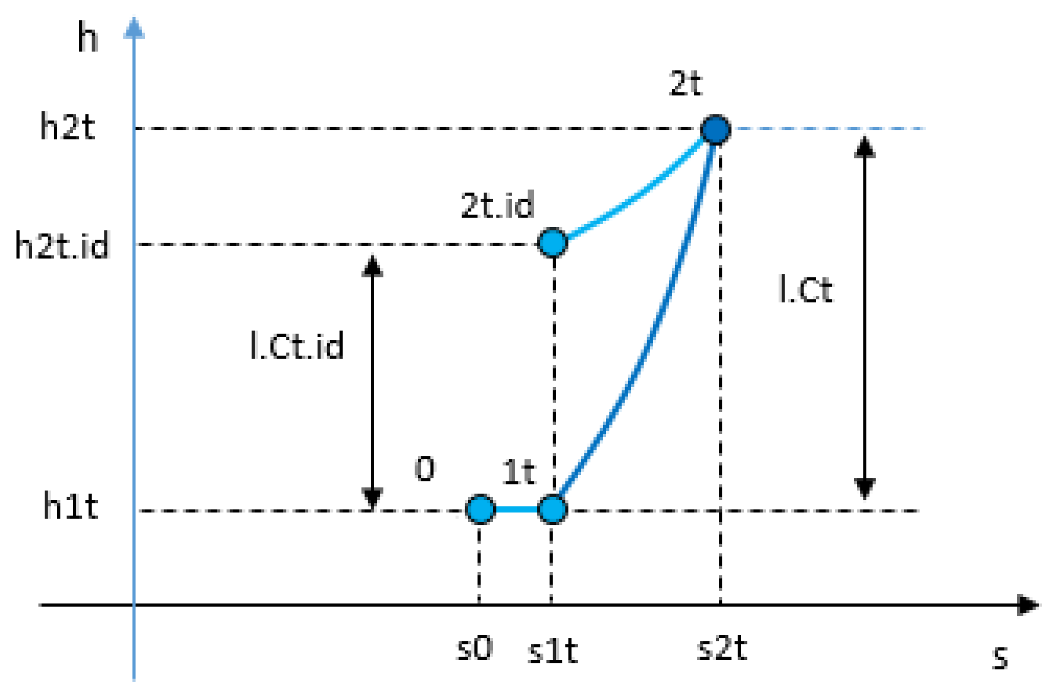
Regarding the expansion process, from the enthalpy–entropy diagram presented in Figure 6, the turbine adiabatic total efficiency is also determined based on the entropy equality conditions [11].

Related to the turbine instrumentation method presented above, and according to the established measurement parameters, the total adiabatic efficiency calculation model is defined by the steps below. Depending on the location of the measured gas temperature, as mentioned above, the inlet turbine gas temperature can be determined from the combustor chamber energy equation [11] in the next form:

$$\begin{array}{ccc}{h}_{3.t}(T_{3.t})=\left(h_{2.t}(T_{2.t})+f_{fc}\cdot LHV\cdot {\eta }_{ca}\right)/\left(1+f_{fc}\right)& \Rightarrow & h_{3.t}(T_{3.t})\end{array}$$

(46)

$$\begin{array}{ccc}{h}_{3.t}(T_{3.t})=i_g\left(T_{3.t}\right)& \Rightarrow & T_{3.t}\end{array}$$

(47)

Therefore, it is necessary to measure the fuel flow ($F_f$) and to know the air mass flow ($M_{af}$) because with these parameters, the fuel flow coefficient ($f_{fc}$), and the gas flow ($G_f$) are determined.

$$f_{fc}=F_f/M_{af}=1/\left({\alpha }_{ex}\cdot {\min }_L\right)$$

(48)

$$G_f=M_{af}+F_f$$

(49)

In case the engine has the inlet turbine temperature measured, and the turbine is on the same spool with the compressor, it is no longer necessary to measure the total outlet temperature, as this temperature can now be calculated. In this case, the calculation model is as follows:

$$\begin{array}{ccc}{h}_{3.t}=i_g\left(T_{3.t}\right)& \Rightarrow & h_{3.t}\end{array}$$

(50)

$$\begin{array}{ccc}{p}_{3.t}=p_{2.t}\cdot {\sigma }_{ca.t}& \Rightarrow & p_{3.t}\end{array}$$

(51)

$$\begin{array}{ccc}{\pi }_{T.t}=p_{3.t}/p_{4.t}& \Rightarrow & {\pi }_{T.t}\end{array}$$

(52)

$$\begin{array}{ccc}{s}_{3.t}=s_g\left(T_{3.t}\right)-R_g\cdot \ln \left(p_{3.t}/p_0\right)& \Rightarrow & s_{3.t}\end{array}$$

(53)

$$\begin{array}{ccc}{l}_{T.t}=l_{C.t}/\left({\eta }_m\cdot \left(1+f_{fc}\right)\right)& \Rightarrow & l_{T.t}\end{array}$$

(54)

In a particular case, for a free turbine turboshaft with a gas generator spool and a power turbine spool, the total specific actual work ($l_{T.t}$) on the whole turbine is the sum between the specific actual work for the gas generator turbine and the free turbine.

$$l_{T.t}=l_{TG.t}+l_{TP.t}$$

(55)

Considering that the power ($P_{TP}$) is measured on the free turbine shaft, the total specific actual work ($l_{T.t}$) is calculated on the free turbine.

$$l_{TP.t}=\frac{P_{TP}}{G_f}$$

(56)

The total specific actual work ($l_{T.t}$) on the gas generator turbine is similar with the next equation.

$$\begin{array}{ccc}{l}_{T.t}=l_{C.t}/\left({\eta }_m\cdot \left(1+f_{fc}\right)\right)& \Rightarrow & l_{T.t}\end{array}$$

(57)

Returning to the general case, the calculation model is as follows:

$$\begin{array}{ccc}{h}_{4.t}=h_{3.t}-l_{T.t}=i_g\left(T_{4.t}\right)& \Rightarrow & T_{4.t}\end{array}$$

(58)

$$s_{3.t}=s_{4.t.id}=s_g\left(T_{4.t.id}\right)-R_g\cdot \ln \left(p_{4.t.id}/p_0\right)$$

(59)

$$\begin{array}{ccc}{s}_g\left(T_{4.t.id}\right)=s_{3.t}+R_g\cdot \ln \left(p_{4.t}/p_0\right)& \Rightarrow & T_{4.t.id}\end{array}$$

(60)

$$l_{T.t.id}=h_{3.t}-h_{4.t.id}=h_{3.t}-i_g\left(T_{4.t.id}\right)$$

(61)

$$\begin{array}{ccc}{\eta }_{T.t}=l_{T.t}/l_{T.t.id}& \Rightarrow & {\eta }_{T.t}\end{array}$$

(62)

In the case of the second instrumentation method, the model calculation for the turbine total adiabatic efficiency is similar to the compressor model and follows the same steps, but it uses the parameters from the outlet and inlet turbine stations.

4.4. Jet Nozzle Total Thrust Calculation Model

Related to the jet nozzle instrumentation method presented above, and according to the established measurement parameters, the engine thrust calculation model is defined by the following steps:

$$\begin{array}{ccc}{M}_5=\sqrt{\frac{2}{k_g-1}\cdot \left[{\left(\frac{p_{5.t}}{p_{5.s}}\right)}^{\left(k_g-1\right)/k_g}-1\right]}& \Rightarrow & M_5\end{array}$$

(63)

$$\begin{array}{ccc}{T}_{5.s}=T_{5.t}/\left(1+\frac{k_g-1}{2}\cdot M_5{}^2\right)& \Rightarrow & T_{5.s}\end{array}$$

(64)

$$\begin{array}{ccc}{h}_{5.t}=i_{5.t}\left(T_{5.t}\right)& \Rightarrow & h_{5.t}\end{array}$$

(65)

$$\begin{array}{ccc}{h}_{5.s}=i_{5.s}\left(T_{5.s}\right)& \Rightarrow & h_{5.s}\end{array}$$

(66)

$$\begin{array}{ccc}{C}_5=\sqrt{2\cdot \left(h_{5.t}-h_{5.s}\right)}& \Rightarrow & C_5\end{array}$$

(67)

$$\begin{array}{ccc}{A}_5=\pi \cdot D_5{}^2/4& \Rightarrow & A_5\end{array}$$

(68)

$$\begin{array}{ccc}F=G_f\cdot C_5+A_5\cdot \left(p_{5.s}-p_0\right)& \Rightarrow & F\end{array}$$

(69)

5. Applied Method of Instrumentation

In this chapter, practical examples of instrumentation methods are presented to determine the main parameters or performances of engine components. The methods were implemented on the Klimov TV2-117A, a free turbine turboshaft, operated in a test bench, as shown in Figure 7. The instrumentation method was used to determine the air mass flow, the compressor total adiabatic efficiency and the turbine total adiabatic efficiency.

In the case of the mass air flow, the engine bellmouth, shown in Figure 8, was fitted with four static pressure probes ($p_s$), and, through a differential pressure transducer in relation to the cell air pressure ($p_0$), the dynamic pressure ($DP$) was measured. The bellmouth diameter is 0.29 (m).

In the case of the compressor adiabatic total efficiency, the first step was to determine the variants of points where the instrumentation probe could be mounted, without making major auxiliary modifications. Then, taking the compressor technical possibilities of being instrumented into account, it was established that the outlet total pressure ($p_{2.t}$) and total temperature ($T_{2.t}$) can be measured at the entry of the combustion chamber’s secondary flow.

Therefore, in this case, the instrumentation was performed by removing two small mounts fixed on the combustion chamber entry section, and it was modified to transform them into instrumentation probes, in order to measure the air total pressure and total temperature [12], as presented in Figure 9.

In the case of the turbine adiabatic total efficiency, because there are not even inspection ports on the turbine case, the turbine instrumentation was conducted by mounting the instrumentation probes [12] in the two holes at the exhaust nozzle entry section. The probes were oriented at the turbine rotor in order to measure the outlet total pressure ($p_{4.t}$) and the outlet total temperature ($T_{4.t}$), as presented in Figure 10. This was possible after small modifications of the holes were made, by mounting the adaptor to connect the instrumentation probes.

In the case of the jet nozzle, this method will be implemented to determine the engine thrust of a Tumansky R-11F2-300, (Tumansky, in URSS (Russia)), turbojet engine, installed on the test bench, as presented in Figure 11, a particular and internal application of the Romanian National Institute of Gas Turbine Engines (COMOTI).

6. Experimental Results

In this chapter, experimental data are presented following the tests performed with the instrumentation methods presented above. The methods were applied to test the TV2-117A engine, a free turbine turboshaft. At takeoff, the TV2-117A turboshaft engine attains a power of ≈1500 HP, a fuel consumption of ≈412.5 (kg/h), an inlet turbine temperature of ≈875 (°C), an overall pressure ratio of ≈6.6:1 and an air mass flow of ≈7.5 ÷ 8 kg/s. The gas generator speed is ≈20,882 rpm (98.5%), and the free turbine speed is ≈11,640 rpm (97%). The engine was tested on various working regimes, defined by the gas generator shaft speed ($N_{GG}$), from idle (64.80%) to a maximum regime (99.11%), so the measured parameters were acquired at each working regime. The experimental values were used in the calculation model presented above in order to determine the mass air flow and the compressor and turbine total adiabatic efficiency. The calculated values are presented in the tables below.

In our case, due to the limited information from the description manual which is provided by the engine manufacturer, the takeoff regime is defined only by the values of shaft speed, power, specific fuel consumption and turbine temperature. Furthermore, the values of the mass air flow, the total overall pressure ratio, the compressor efficiency and the turbine efficiency are not provided. Therefore, in order carry out a comparison between the engine measured main parameters and the data from the manufacturer manual, it can be performed only at the takeoff regime. According to the engine manual [13], the takeoff regime is defined by the next values of performances and main parameters from

Table 4. Engine data for takeoff regime, based on the engine manual.

Data from Manual at Sea Level Conditions$T_0=15 °\mathrm{C}$, $p_0=1.01325\mathrm{bar}\mathrm{a}$
Takeoff regime	$N_{GG}[\%]$	$P[\mathrm{kW}]$	$F_f[\mathrm{kg}/\mathrm{s}]$	$T_{3.t}[°\mathrm{C}]$	${\pi }_{C.t}\left[\text{-}\right]$	$M_{af}[\mathrm{kg}/\mathrm{s}]$
	98.5	1103	0.1145	875	-	-

and

Table 5. Engine data for takeoff regime, based on outside sources.

Data from Other Sources at Sea Level Conditions$T_0=15 °\mathrm{C}$, $p_0=1.01325\mathrm{bar}\mathrm{a}$
Takeoff regime	$N_{GG}[\%]$	$P[\mathrm{kW}]$	$F_f[\mathrm{kg}/\mathrm{s}]$	$T_{3.t}[15 °\mathrm{C}]$	${\pi }_{C.t}\left[\text{-}\right]$	$M_{af}[\mathrm{kg}/\mathrm{s}]$
	-	1103	0.1145	807 1	6.6	Max 8.0

¹ In this case, the turbine temperature value (807 °C) was determined with the above values for the mass air flow and overall pressure ratio.

shows engine main parameters from outside sources [14,15].

In the case of our application, with the engine running on the test bench, we obtained the next values of the main parameters presented in

Table 6. Measured and calculated parameters at maximum working regime on the test bench, part one.

Parameter Measured				Parameter Calculated	Parameter Measured		Parameter Calculated
$N_{GG}[\%]$	$T_0[°\mathrm{C}]$	$p_0\left[\mathrm{bar}\mathrm{a}\right]$	$DP\left[\mathrm{mbar}\right]$	$M_{af}[\mathrm{kg}/\mathrm{s}]$	$p_{2.t}\left[\mathrm{bar}\mathrm{a}\right]$	$T_{2.t}\left[\mathrm{K}\right]$	${\pi }_{C.t}[\text{-}]$	${\eta }_{C.t}\left[\text{-}\right]$
99.11	24.3	1.004	64.000	7.436	6.200	540.6	6.225	0.830

and

Table 7. Measured and calculated parameters at maximum working regime on the test bench, part two.

Parameter Measured		Parameter Calculated	Parameter Measured		Parameter Calculated
$N_{GG}[\%]$	${\mathrm{F}}_f[\mathrm{kg}/\mathrm{s}]$	$G_f[\mathrm{kg}/\mathrm{s}]$	$T_{3.t}\left[\mathrm{K}\right]$	$\mathrm{P}\left[\mathrm{kW}\right]$	$p_{4.t}\left[\mathrm{bar}\mathrm{a}\right]$	$T_{4.t}\left[\mathrm{K}\right]$	${\pi }_{T.t}[-]$	${\eta }_{T.t}[\text{-}]$
99.11	0.109	7.545	1140.0	1027.5	1.069	783.5	5.627	0.833

.

7. Discussion

One of the advantages of our methods is that each parameter in the calculation algorithm is calculated successively, with the purpose of determining the main parameters. For instance, the mass air flow was not preferred to be defined as an explicit global formula because only the flow will be determined, and in our case, the determination of all parameters was aimed at. For the same reason, it was applied on most of the engine main parameters.

To compare the measured data that were obtained at 24.3 °C and 1.004 bar absolute with the calculated data and the data from the manual [13], it is necessary to correct [11] the measured data with temperature and pressure from the sea level standard atmospheric condition ($T_0=15 °\mathrm{C}$, $p_0=1.01325 \mathrm{bar} \mathrm{a}$). The corrected results from our analysis are presented in the

Table 8. The corrected measured data.

Takeoff regime	$N_{GG.cr}[\%]$	$P_{.cr}[\mathrm{kW}]$	$F_{f.cr}[\mathrm{kg}/\mathrm{s}]$	$T_{3.t.cr}[°\mathrm{C}]$	${\pi }_{C.t.cr}\left[\text{-}\right]$	$M_{af.cr}[\mathrm{kg}/\mathrm{s}]$
	97.54	1053.5	0.1083	849	6.25	7.624

and

Table 9. Percentage difference values.

Takeoff regime	$\Delta N_{GG}[\%]$	$\Delta P[\%]$	$\Delta F_f[\%]$	$\Delta T_{3.t}[\%]$	$\Delta {\pi }_{C.t}[\%]$	$\Delta M_{af}[\%]$
	1.0	−4.5	−5.4	3.0	4.1	−4.7

below.

Therefore, the engine measured and calculated main parameters, such as power, fuel flow, total turbine temperature and mass air flow, can be compared with the data from the manufacturer data by using the differences in percentage values which are defined by the next equations [16].

$$\Delta P=\frac{P_{cr}}{{(P)}_m}\cdot 100-100[\%]$$

(70)

$$\Delta F_f=\frac{F_{f.cr}}{{(F_f)}_m}\cdot 100-100[\%]$$

(71)

$$\Delta T_{3.t}=\frac{T_{3.t.cr}}{{(T_{3.t})}_m}\cdot 100-100[\%]$$

(72)

$$\Delta M_{af}=\frac{M_{af.cr}}{{(M_{af})}_m}\cdot 100-100[\%]$$

(73)

From these results, it can be observed that the higher difference is 5.5% and the rest are lower than 5%. From this, it can be noted that the limit error of acceptability is exceeded marginally.

It is to be noted that, for the calculated data, except the bellmouth which has four instrumentation points, because of the engine’s limited possibilities to be instrumented, the compressor and turbine have only one instrumentation point for each measured parameter. In this case, the parameter values for each working regime are defined only by one measure point. If a comparative study of the measured values is carried out and it is observed that the values from the engine manual are close to the measured ones, it will mean that the above-described method can be used and is already available to be applied.

8. Conclusions

This paper presents an applied method of instrumentation and applied calculation methods to determine specific engine main parameters or performances of the engine components, such as the compressor, turbine and jet nozzle. Depending on the engine type, turboshaft or turbojet, additional instrumentation on the engine is involved, in order to determine the main parameters or performance. The parameters mean a series of thermodynamic parameters, pressure and temperature, in the main engine stations, more precisely, in the sections that define the input and output of the engine inlet, compressor, turbines, exhaust nozzle or jet nozzle. In accordance with the request for the specific parameters which must be determined, this paper shows the steps of a gas turbine supplementary instrumentation, starting from the study on how accessible is the engine to be instrumented, the study of what parameters can be measured and the possibility of installing the instrumentation probes, and ending with the main parameters and performance model calculation for each applied instrumentation method, based on the various measured data. By testing the engine on a test bench, a series of experimental results were obtained, which were analyzed and compared with reference values from the engine manual. It was determined that the values from the test and from the manual are very similar, which means that instrumentation methods and model calculations are available to be applied and implemented on other engines as well.

References

- SAE ARP 1217A. Instrumentation Requirements for Turboshaft Engine Performance Measurements; Aviation Standards; SAE International: Warrendale, PA, USA, 1 May 1997. [Google Scholar]
- SAE ARP 1587. Aircraft Gas Turbine Engine Monitoring System Guide; Aerospace Recommended Practice; SAE International: Warrendale, PA, USA, April 1981. [Google Scholar]
- Available online: https://www.vzlu.cz/en/engineering-for-gas-turbine-engines-c272.html#prettyPhoto (accessed on 11 May 2021).
- Available online: https://www.ciam.ru/en/experimental-bases/ (accessed on 11 May 2021).
- SAE AIR 1873. Guide to Limited Engine Monitoring Systems for Aircraft Gas Turbine Engines; Aerospace Information Report; SAE International: Warrendale, PA, USA, May 1988. [Google Scholar]
- Purvis, J.T. Industrial Gas Turbine Performance Measurement, International Congress on Combustion Engines; Texas A&M University: College Station, TX, USA, 1974. [Google Scholar]
- Available online: https://www.bkvibro.com/fileadmin/mediapool/Internet/Application_Notes/Gas_Turbines_BAN0010EN12.pdf (accessed on 11 May 2021).
- Saravanamuttoo, H.I.H. Recommended Practices for Measurement of Gas Path Pressures and Temperatures for Performance Assessment of Aircraft Turbine Engines and Components; Theory of Gas Turbine, AGARD Advisory Report Number 245; Advisory Group for Aerospace Research and Development (AGARD): Neuilly sur Seine, France, 1990. [Google Scholar]
- Cohen, H.; Rogers, G.F.C.; Saravanamuttoo, H.I.H.; Mayhew, Y.R. Gas Turbine Theory, 4th ed.; Longman Group Limited: London, UK, 1996. [Google Scholar]
- Stanciu, V. Jet Engines Preliminary Design Guide, Polytechnic Institute of Bucharest, Aircraft Faculty, Gas Turbine Theory, Course Notes; Polytechnic Institute of Bucharest: Bucharest, Romania, 1991; (Translation from Romanian). [Google Scholar]
- Bathie, W.W. Fundamentals of Gas Turbines; Iowa State University of Science and Technology: Ames, IA, USA, 1984. [Google Scholar]
- Anthoine, J.; Arts, T.; Boerrigter, H.L. Measurement Techniques. In Fluid Dynamics, 3rd ed.; Von Karman Institute for Fluid Dynamics: Genesius-Rode, Belgium, 2009; ISBN 978-2-930389-96-6. [Google Scholar]
- Zambfirescu, V. TV2-117A Free Turbine Turboshaft Engine Description and Maintenance Manual, Engine Maintenance; Documentation and Technical Publications Center: Bucharest, Romania, 1973; (Translation from Romanian). [Google Scholar]
- Available online: http://all-aero.com/index.php/64-engines-power/13152-klimov-tv2-117-isotov-tv2-117 (accessed on 11 May 2021).
- Available online: http://etexportbg.com/en/catalog/aviation/engines.html (accessed on 11 May 2021).
- Available online: https://www.onlinemathlearning.com/relative-error-formula.html (accessed on 11 May 2021).
Figure 1.
Bellmouth instrumentation method scheme, model (a), bellmouth instrumentation method scheme, model (b).
Figure 2.
Compressor instrumentation method scheme, model (a); compressor instrumentation method scheme, model (b).
Figure 3.
Turbine instrumentation method scheme, model (a); turbine instrumentation method scheme, model (b).
Figure 4.
Jet nozzle instrumentation method scheme.
Figure 5.
Compressor enthalpy–entropy diagram.
Figure 6.
Expansion enthalpy–entropy diagram.
Figure 7.
TV2-117A installed on test bench.
Figure 8.
TV2-117A bellmouth instrumentation.
Figure 9.
Compressor total outlet temperature probe (a); compressor total outlet pressure probe (b); compressor total outlet temperature probe location (c); compressor total outlet pressure probe location (d).
Figure 10.
Free turbine total outlet pressure and temperature probe (a); free turbine total outlet temperature probe location (b).
Figure 11.
R-11F2-300 turbojet engine on the test bench.