Abstract
In order to meet the requirement for the real-time of the hydraulic walking robot (WLBOT) and the stability of its movement, an embedded controller is proposed, which takes charge of multi-sensor information processing and signal output of the servo valve. The controller is capable of receiving control command and sending processed information while communicating with an embedded single board computer PCM-3365 via Control Area Network (CAN) bus at a 200 Hz frequency. In this paper, an appropriate interrupt cycle is selected and a 2 kHz high-speed control loop is run after we research the relationship between analog-to-digital converter direct memory access (ADC–DMA) interrupt cycle, data volume, and sampling rate. Significantly, the control strategy of WLBOT joint is introduced and a proportional-integral-derivative (PID) compound controller with velocity feedforward compensation (VFC) is realized. Meanwhile, the Chebyshev filtering algorithm is utilized to attenuate the vibration noise of joint signals. What’s more, an impedance controller is designed to gain better locomotion behavior and compliance in joint force control. Finally, the joint angle tracking and robot walking experiments are implemented, where the feasibility of the design and the validity of the control algorithm is verified. The results show that the PID velocity feedforward compensation controller can reduce the maximum tracking error by 39.13% and 71.31% in the knee and hip joint and the impedance control can reduce the standard deviation (SD) of the foot force by 36.06% and 72.79%.
1. Introduction
Over the past decades, multilegged robots have gained more and more attention for their ability to traverse nonstructural environments and uneven terrains like mammals or insects. Furthermore, they not only can play an important role in transporting materials on flat or rough terrain but also can execute many dangerous missions alone or in cooperation with humans, such as outdoor exploration, disaster rescue, and dangerous substance detection [1]. Compared with the electric actuators, hydraulic actuation can provide extremely high power density, fast dynamic response, large force output, and strong robustness to impacts [2], which are widely used in hydraulic robotic manipulators [3]. Thus, hydraulic legged robots apply to more and more heavy load occasions [4]. Boston Dynamics developed hydraulic quadruped or humanoid robot series, including BigDog [5], LS3, Cheetah, Wildcat, Petman [6], Handle, Atlas [7], which brought the topic into a hotspot. Italian Institute of Technology (IIT) constructed a series of high-performance hydraulic quadruped robots, such as HyQ [8], miniHyQ [9], HyQ2Max [10], HyQReal. Korea Institute of Industrial Technology (KITECH) proposed hydraulic quadruped robots qRT-1, qRT-2 [11], p2 [12], and JINPOONG [13]. Meanwhile, Shandong University’s (SDU) quadruped robots SCalf-I [14], SCalf-II [15], and SCalf-III [16], Shanghai Jiao Tong University’s (SJTU) Baby elephant [17] and Octopus [18], Harbin Institute of Technology’s (HIT) MBBOT [19], National University of Defense Technology’s (NUDT) quadruped robot [20] and Beijing Institute of Technology’s (BIT) bionic quadruped robot [21] also continued to obtain advances in the fields of dynamic locomotion and control in recent years.
Since legged robots usually need to implement multiple tasks at the same time, such as data collection, posture calculation, gait planning, actuation control, they often adopt a hierarchical control system, where the embedded controller often plays an important role. BigDog is controlled by a layered onboard computer that contains a PC104 Pentium processor (Intel Corporation, Santa Clara, California, U.S.) running a multi-rate real-time operating system under QNX as well as I/O cards and I/O interfaces. The high-level control system coordinates the behavior of the legs to regulate the velocity, attitude, and altitude of the body during locomotion in 200 Hz while the lower-level control system servos positions and forces at the joints in 1 kHz [22]. HyQ’s control system architecture consists of a CPU board and five multifunction I/O boards. The CPU board is a Kontron MOPSPM104 board (Kontron S&T AG, Augsburg, Germany) running a real-time patched version of Linux (Linux kernel patched with real-time Xenomai), while five multifunction I/O boards are responsible for four legs and other sensors in a 1 kHz control frequency [23]. qRT-2 has a control architecture composed of the task level controller, the function level controller, the local controller, and the power controller [11]. The MIT Cheetah, whose control system is comprised of four layers: the motor drivers, the parallel UART emulators, the real-time multicore controller, and the monitoring PC, uses an i7 dual-core 1.33 GHz CPU as the real-time controller running two 4 kHz high priority loops [24]. ANYmal has three Intel NUC PCs (Intel Corporation, Santa Clara, California, U.S.) running the robot operating system (ROS) with a 400 Hz actuator control frequency, including inspection PC, navigation PC, and locomotion PC [25]. SCalf has a control system comprised of an industrial personal computer and a TMS320f28335 digital signal processor (DSP) (Texas Instruments Incorporated, Dallas, Texas, U.S.) with a 5 kHz sampling frequency and 1 kHz servo rate [26]. MBBOT owns a PC104 main controller and four leg servo controllers with a 1 kHz joint control frequency [27]. Chapuis et al. developed a low-cost FPGA-based decentralized control system for a MEMS-based distributed air-flow micromanipulator [28].
Dynamic motions of the legged robots have been studied for years, and many control methods have been proposed. HyQ uses dynamic torque control to be actively compliant, with an inner PID torque loop and an outer PID position loop [29]. It also proposes a position control combined with an admittance block to handle the environmental interaction efficiently while the robot is trot-walking [30]. MIT Cheetah I is controlled by the proprioceptive impedance controller to achieve a stable gallop at 3.2 m/s which can allow reflex responses to external forces according to the predefined compliance [31]. ANYmal develops a cascaded joint torque, position, and impedance control to realize the joint tracking very accurately [32]. JINPOONG uses a PD plus feed-forward controller to walk stably on uneven terrain [33]. Chen et al. utilized a virtual model control (VMC) in SCalf-II to reduce the contact force by 35.7% [15]. Zhang et al. designed a position/force control law on the base of the operation space dynamic equation and the maximum sinusoid tracking error was less than 8 mm [34]. Zhang et al. acquired a foot contact estimation method in the impedance control and proposed a compensation scheme using neural network in the real quadruped robot system [35]. Xie et al. presented a VMC for quadrupedal dynamic locomotion, which consisted of a stance phase virtual model control for full control of the robot body and a swing phase virtual model control for control of swing legs [36]. Chen et al. proposed an impedance controller to solve the ball-on-plate (BoP) problem for six-parallel-legged robots walking on irregular terrains based on seven six-dimensional(6D) force/torque(F/T) sensors [37]. Wirekoh et al. implemented a real-time position and force feedback control for the artificial muscle with microfluidic sensors [38]. Cairone et al. presented a PDMS micro-optofluidic chip [39] and identified a class of models representing the two-phase microfluidic flow in different experimental conditions [40].
This paper gives an introduction of the quadruped hydraulic wheeled-legged robot WLBOT, including its structure, hydraulic system, and control system. It concentrates on the embedded controller, including the hardware, software design, and control strategy. Both the joint position control and joint force control are introduced respectively. In joint position control, a PID controller with velocity feedforward compensation (VFC) is proposed and the Chebyshev filtering algorithm is utilized to reduce the impact of joint jitter. What’s more, an impedance controller is designed to realize better locomotion behavior in joint force control. Finally, the test platform is constructed, where the feasibility of the design and the validity of the control algorithm is verified. This paper makes the following contributions:
- The relationship between ADC-DMA interrupt cycle, data volume, and the sampling rate is researched and a 2 kHz high-speed control loop for the embedded controller is proposed to realize better control performance;
- A proportional-integral-derivative (PID) velocity feedforward compensation (VFC) controller is designed to realize the joint position control. Compared with the general PID, VFC can reduce the maximum joint tracking error by 39.13% and 71.31%;
- The Chebyshev filtering algorithm is utilized to reduce the vibration noise of joint signals;
- An impedance controller in the joint space is proposed to get the better locomotion behavior and compliant effect in the walking experiments.
2. WLBOT System Overview
2.1. WLBOT Structure and Onboard Hydraulic System
The hydraulic walking robots can walk in different gaits to overcome irregular terrains and obtain better environment adaptability, higher stability, and larger load capacity. WLBOT has a size of about 1.1 m (L) × 0.72 m (W) × 1.0 m (H) at the standard standing position and a total of about 220 kg weight with an extra load capability of about 50 kg. As is shown in Figure 1, the robot consists of a trunk and four legs, while two front legs both have a three-DOF structure and two hind legs only own a retractable joint with a wheel. Each front leg of WLBOT adopts the same mechanism, which consists of three DOFs (degree of freedom) to meet the locomotion requirement, including root abduction/adduction (RAA), hip flexion/extension (HFE) [29], and knee flexion/extension (KFE). The driving hydraulic cylinders for the hip joint and knee joint are fixed on the thigh, while the root joint cylinder is set on the pelvis, as depicted in Figure 1. Furthermore, WLBOT has two spring damping feet, which can attenuate the shock and vibration and thus improve the energy utilization during the locomotion.

Figure 1.
The quadruped wheeled-legged robot WLBOT. (RAA: root abduction/adduction; HFE: hip flexion/extension; KFE: knee flexion/extension.).
In order to meet the requirements of heavy load and motion stability of the hydraulic walking robot, each joint unit uses a valve-controlled hydraulic cylinder as its actuator. There are eight joint units in the onboard hydraulic system. The hydraulic pressure is generated by an internal gear pump connected to a relief valve with an adjustable pressure range of 2 to 31.5 MPa. The flow rate of the hydraulic system can be adaptive because the speed of the pump is controlled by a servomotor. The accumulator provides extra flow if needed and reduces pressure fluctuation. All components are powered by a 48 V–100 Ah lithium battery. The manifolds are made of aluminum alloy to reduce mass. A schematic of WLBOT onboard hydraulic system is illustrated in Figure 2 where only two joint units are displayed and the other six joint units are omitted.

Figure 2.
Schematic of WLBOT hydraulic system.
2.2. WLBOT Control System Architecture
According to the characteristics of WLBOT, such as a large number of sensors, high real-time requirements, and complex complicated control strategy calculation, we establish a hierarchical control system. From top to bottom, they are management level, coordination level, and execution level. Firstly, a remote personal computer (PC) works as a management level, which can provide an interactive interface and WiFi communication. Secondly, an industrial personal computer PCM–3365 (Intel Corporation, Santa Clara, California, U.S.) behaves as the coordination level, which will complete gait planning, trajectory planning, and communication in CAN bus and WiFi module. What’s more, PCM–3365 also processes information from a camera, a global positioning system (GPS), and an inertial measurement unit (IMU). Finally, the execution level is three embedded controllers. The configuration of the hierarchical control system is shown in Figure 3. Both the PCM–3365 and three embedded controllers are placed inside the robot trunk.

Figure 3.
Configuration of the hierarchical control system. (PC: personal computer; GPS: global positioning system; IMU: inertial measurement unit; LF leg: left front leg; RF leg: right front leg.).
3. Embedded Controller Hardware Design
As is displayed in Figure 3, the embedded controller meets both functional requirements and nonfunctional requirements.
- Each embedded controller needs to sample each joint angle and angular velocity, two chambers’ pressure, system pressure, and foot force, a total of 14 sensor signals. After that, A/D converting and signal processing will be implemented.
- The embedded controller can receive joint angle command from PCM–3365 and give 14 processed sensor signals back to it via CAN bus.
- The control algorithm and D/A converting will be calculated to realize the position servo control of each joint.
- The embedded controller can run a 2 kHz high control frequency.
- Each controller can communicate with PCM–3365 in 200 Hz via CAN bus, while this frequency is determined by PCM–3365.
- The sampling voltage range is 0 V~+5 V, while the sampling resolution reaches 0.1%. and the sampling rate reaches 300 kHz. The output voltage range is −10 V~+10 V.
In order to meet all these requirements above, we develop an embedded controller based on STM32F407ZGT6 ARM chip as Figure 4 depicts. The hardware includes a CAN bus module, a sensors module, a DAC output module, a data storage module, a DC–DC power module, and other peripheral circuits.

Figure 4.
The hardware structure of the embedded controller.
The electrical connections of the embedded controller are shown in Figure 5. Three encoders are mounted in the joints to measure the joint angles. A force sensor is mounted on the foot of the robot foot to measure the ground contact force. Seven pressure gauges are mounted on the manifold to measure the pressure of the cylinder chamber as well as the system pressure. When the robot is walking, the control inputs are calculated and the voltage outputs are sent to the servo valves through a D/A converter which is used to drive the joints of the hydraulic cylinders. The angular velocity adopts a secondary amplifier differential circuit and both cut-off frequencies are 72.3 Hz, while other sensor signals adopt the same first-order filtering circuit whose cut-off frequency is 241 Hz.

Figure 5.
Electrical connections of the embedded controller.
4. Embedded Controller Software Design
4.1. Software Architecture
As the essential part of the control system, the software component is supposed to take responsibility for the reasonable arrangement of multiple tasks. The control frequency of the embedded controller affects the accuracy and stability of the robot control. It’s vital to utilize the CPU resources effectively, select the interrupt cycle and configure the priority reasonably. The software program consists of the main program module and four interrupts, which are shown in Figure 6 and Figure 7. The interrupt priority is configured in Table 1 and makes the interrupt service routine (ISR) run properly.

Figure 6.
The flow chart of the main program.

Figure 7.
The flow chart of ISR.

Table 1.
Configuration of interrupt priority.
The flow chart of the main program is shown in Figure 6. When the embedded controller is powered on, the main program will start. The initialization will be implemented firstly and CAN receive interrupt will also be enabled to wait for a command from PCM–3365. When the controller gets a start command, it will set the flag ‘Start’. After that, both ADC1 and ADC3 sampling and interrupt will be enabled as well as the control interrupt. Then the main program will be waiting for the interrupt until the stop command comes. When it comes to the stop command, all the interrupts and ADC sampling will be disabled and the DAC output will be set to zero to avoid servo valves’ misoperation. Before the end, all the test data will be copied from the external SRAM to the SD card for further study.
There are four interrupts as Table 1 shows and the flow chart of ISR is illustrated in Figure 7. When the CAN receive interrupt comes, the controller reads data from PCM–3365 and makes different responses according to different commands. Especially, when it gets a start command, the control strategy will be stored. In ADC1–DMA and ADC3–DMA interrupt, the sampling data will be processed in the median and mean filtering. After that, the processed data will be stored in the temporary arrays for the control algorithm to use. As for the control interrupt, the control algorithm will be calculated and all the processed data will be stored in external SRAM for further use.
4.2. Research on the Relationship Between ADC-DMA Interrupt Cycle, Sampling Data Volume, and ADC Sampling Rate
As we need to sample 14 sensor signals, we select both ADC1 and ADC3 controllers while each controller can offer seven sampling channels. ADC1 selects DMA2 stream0 and ADC3 selects DMA2 stream1. When it comes to a start command from PCM–3365, the embedded controller starts continuous sampling. When the data buffer of each DMA is full, an interrupt will be triggered. For the configuration of DMA in ADC sampling, we can reduce the burden of CPU, which greatly improves the embedded controller’s efficiency.
For STM32F4 series chips, the total ADC conversion time is calculated as follows:
Tcv = Sampling time + 12 cycles
The shortest sampling time can be configured as three cycles. Though the extension of the sampling time will improve the accuracy of sampling, it reduces the AD conversion rate. Since the maximum frequency of STM32F407ZGT6 is 168 MHz, to ensure the accuracy of sampling, ADCCLK prescaler is configured to a division factor of 4, and thus the maximum sampling clock frequency is 21 MHz.
The ADC–DMA interrupt cycle can be calculated as follows:
where is the number of ADC sampling channels, is the sampling data volume of each channel when the data buffer of DMA is full, and is the actual sampling rate.
Our primary selection is . With the online debugging function of Keil uVision 5, we can estimate that the third-order median and mean filtering in DMA interrupt costs about . Thus, the average processing time for each data is about . If each DMA channel stores data, it will cost as follows:
td = Ndt1 = 5d × 10−6 s
Besides filtering, other programs in DMA interrupt only cost about . So the ADC–DMA interrupt service routine cost about as:
tt = (5d × 10−6 + 1 × 10⁻⁵) s
Since the running time of the DMA interrupt service routine must be less than or equal to the ADC–DMA interrupt cycle:
tt ≤ Tit
Combine Equations (2), (3) and (5), we can easily get the maximum ADC sampling rate and the minimum ADC–DMA interrupt cycle :
According to Equation (6), we can plot the relationship between the minimum ADC–DMA interrupt cycle , the maximum ADC sampling rate , and the sampling data volume in Figure 8.

Figure 8.
Relationship between , and .
In the ADC–DMA interrupt, the sampling data will be processed in the median and mean filtering. It has been tested that the filtering algorithm time occupies most of the DMA interrupt service routine time. When is nearly unchanged, will be shorter as gets smaller. However, when is too small, it will worsen the filtering effect and reduce . As a result, after coordinating the relationship between , and , we choose an appropriate ADC–DMA interrupt cycle and obtain better sampling results. The final parameters , actual sampling rate , and actual ADC–DMA interrupt cycle are shown in Equation (7). By using the oscilloscope, we can observe that both ADC1–DMA and ADC3–DMA interrupt cycles are about , which is consistent with the theoretical analysis.
4.3. Realization of High-Speed Control Frequency
PCM–3365 can only send 200 Hz commands via CAN bus, which is far from meeting the requirement of the motion control. Thus, we need to use the previous and the current commands sent by PCM–3365 to perform Lagrangian interpolation in the CAN receive interrupt. The Lagrangian polynomial is obtained and converted into the form required by the embedded controller, as shown in Equation (8).
where is the interpolated joint angle command, and is the previous and current joint angle command, .
With the help of Lagrangian interpolation, nine values are inserted between the two commands sent by the PCM–3365, and the interval between the new interpolated commands is , which is consistent with the 2 kHz control frequency. The embedded controller utilizes to perform control algorithm calculation during the control interrupt to achieve high-speed control frequency.
With the configuration of interrupt priority, it is ensured that the control interrupt has the highest priority, and the control interrupt and CAN receive interrupt can interrupt the ADC1–DMA and ADC3–DMA ISRs. Since DMA interrupt cycle is shorter than control interrupt cycle, the latest data is continuously written in the CAN send array in ADC–DMA ISRs. As a result, in the control interrupt, we make sure that the control algorithm can always utilize the latest information obtained by the sensors, which is vital to the real-time control of the robot.
Due to the existence of interrupt nesting, we introduce a temporary storage array in ADC–DMA ISRs to reduce the impact of data loss if the filtering program is interrupted. Take ADC1–DMA interrupt as an example. When it comes to the ADC1–DMA ISR, we firstly perform median and mean filtering on the 20 data collected by each channel. Then the processed data for one channel will be temporarily stored in the temporary storage array. Finally, after all the data in seven channels is processed, we transfer all the data in a temporary storage array to the CAN send array for the control algorithm to use. In this case, the data in the CAN send array will be sent to PCM–3365 in the next CAN receive interrupt. The calculation of the control algorithm utilizes the interpolated commands and data in the CAN send array. Even if the executing filtering ISR is interrupted, we can’t get the current complete ADC sampling data, we can still use the last ADC sampling data stored in the CAN send array to implement the control algorithm. Considering the current data and the last data just has a difference of about , the influence can be omitted.
The running time of four ISRs is tested through an oscilloscope, as shown in Table 2. It’s obvious that the control interrupt ISR is much shorter than the interrupt interval, which will reserve enough space for more complex control algorithms in the future.
Table 2.
Running time of ISR.
4.4. Joint Control Algorithm
4.4.1. PID Control with Velocity Feedforward Compensation (VFC)
In order to realize joint position control, we develop a PID (proportional-integral-derivative) compound controller with velocity feedforward compensation (VFC) as Figure 9 illustrates.

Figure 9.
The block diagram of VFC.
The compound controller consists of a conventional PID controller and velocity feedforward compensation (VFC). The control law is shown in Equation (9).
where is the tracking error; is the desired angle; is the feedback angle; , , are the proportional gain, integral gain, and derivative gain; is the desired angular velocity; is the velocity compensation gain.
4.4.2. Design of Chebyshev Digital Filtering Algorithm
In the double-joint step response experiment, it is found that the joint jitter is greater in the steady state. Analyzing the experimental data, it is the large fluctuation of the derivative term of the PID output which causes the phenomenon. Although we can use a smaller PID coefficient to reduce the influence of joint jitter, it will bring about the longer settling time. Thus, we consider using the digital low-pass filtering of the derivative term in the PID controller to increase the stability of the robot in the steady state without reducing its response speed. Chebyshev I Filter is introduced in Equation (10).
where is a positive number less than 1, is the passband boundary frequency.
We can design a Chebyshev I Filter as Equation (11) shows, with a 70 Hz cut-off frequency. When we convert the Z transfer function into a difference equation, we can implement it in the embedded controller.
4.4.3. Impedance Control
Since hydraulic walking robots are typically modeled as rigid body systems, they have forces or torques as input to their dynamics, and therefore being able to apply precise joint torques to a robot has many advantages. Contrary to the position control, impedance control, as one of the force controls, can significantly increase the versatility and compliance of the robot, which will have outstanding advantages in the interaction with the environment, especially in the walking experiment. The general concept of impedance control was introduced by Hogan in the seminal work [41,42] and can nowadays be considered as a classical control approach in robotics. Thus, we design a joint impedance controller in the joint space as Figure 10 shows. The force inner loop PID controller adopts the same form of the first row of Equation (9). The impedance control can be described as a virtual spring-damper system or a PD controller, which acts as the position outer loop. The control law and the feedback are shown in Equation (12).
where and are the stiffness and damping of the virtual joint spring; and are the error of angle and angular velocity; and are the acting area of piston and rod chamber; and are the pressure of piston and rod chamber; is the force arm of output force of the joint hydraulic cylinder.

Figure 10.
The block diagram of impedance control.
5. Experiment
5.1. Chebyshev Digital Filtering Algorithm
Analyzing the data obtained from the double-joint step response experiment, the PID output voltage value of the derivative term is shown in Figure 11 below. Comparing the unfiltered derivative term with the derivative term after Chebyshev filtering, it is found that, for high-frequency interference, the designed digital filter has a good effect to get the smoother control command output, which greatly attenuates the vibration noise and enhances the steady state stability.

Figure 11.
Derivative term before and after Chebyshev filtering algorithm: (a) knee PID output; (b) hip PID output.
5.2. Joint Angle Tracking
The robot is tested by performing an offline joint trajectory tracking task, in which we compare the general PID controller and the compound PID controller with velocity feedforward compensation as Figure 12 depicts. The PID gains and the velocity compensation gain are shown in Table 3. With the control of a single PID controller, the maximum tracking errors of the knee and hip angles are 0.092 rad and 0.122 rad in a gait cycle. However, when using the compound PID controller, the maximum tracking errors decrease to 0.056 rad and 0.035 rad, reduced by 39.13% and 71.31% respectively, which has obvious improvement. Furthermore, the comparison of mean and standard deviation (SD) of tracking errors are compared in Table 4.

Figure 12.
Comparison of two controllers in joint trajectory tracking and error: (a) knee trajectory; (b) hip trajectory; (c) knee tracking error; (d) hip tracking error.
Table 3.
PID gains and velocity compensation gain.
Table 4.
Comparison of PID and VFC tracking errors.
5.3. Impedance Control Walking Experiment
The impedance control performance is tested in a walking experiment, where WLBOT is moving at a speed of 0.5 m/s and the gait cycle is 2 s. The control performances of the position outer loop and the force inner loop are shown in Figure 13, where the coefficients of impedance control are shown in Table 5. The maximum tracking errors of the knee and hip angles are 0.058 rad and 0.146 rad, while the mean and SD of the position and torque tracking are given in Table 6. Compared with the joint position control, the impedance control needs a position error to create the desired torque . But on the other hand, the fluctuation of foot force can be decreased as Figure 14 depicts, which is consistent with the actual situation. Table 7 shows that the SD of foot force on the left and right in the robot stance phase can be reduced by 36.06% and 72.79% in the impedance control, compared with the position control. In the walking experiment, the impedance control shows great advantages for the virtual spring-damper can achieve a good compliant effect on the actual system.
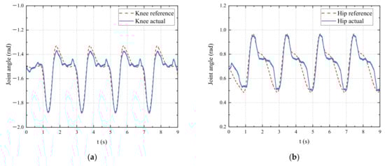

Figure 13.
Control performance of the position outer loop and the force inner loop: (a) knee trajectory; (b) hip trajectory; (c) knee torque; (d) hip torque.
Table 5.
Impedance control coefficients.
Table 6.
Comparison of position and torque tracking errors.

Figure 14.
Comparison of the foot force between impedance control and position control.
Table 7.
Comparison of data of the foot force between impedance control and position control.
6. Conclusions and Future Work
This paper focuses on the design and control strategy of an embedded controller for the hydraulic quadruped robot WLBOT. First, an overview of the WLBOT is given, including its mechanical structure, onboard hydraulic system, and hierarchical control system. Then an embedded controller for WLBOT is designed in detail. The embedded controller’s hardware consists of a CAN bus module, a sensors module, a DAC output module, a data storage module, a DC–DC power module, and other peripheral circuits. In the software design, the main program and four interrupts are introduced as well as their flow charts. CAN receive interrupt will finish the information communication with PCM–3365, while ADC–DMA interrupt can sample and process 14 sensor signals and control interrupt will realize the complex control algorithm. By studying the relationship between ADC–DMA interrupt cycle, data volume, and sampling rate, we select an appropriate interrupt cycle to achieve the controller’s 2 kHz high-speed control frequency. Then the joint position control PID VFC is proposed, combined with the Chebyshev filtering algorithm to reduce the impact of joint jitter. Furthermore, an impedance controller in the joint space is designed to realize better locomotion behavior in the walking experiment. Finally, the experiments show that PID VFC control can have better joint position control accuracy, which can reduce the maximum tracking error by 39.13% and 71.31%. In the walking experiment, the impedance control can achieve a good compliant effect and reduce the SD of foot force by 36.06% and 72.79%, compared with the position control.
Future work will concentrate on improving the motion ability of the robot as well as other complex control strategies for the position, force, and hydraulic system.
Author Contributions
Conceptualization, Z.L., C.Z., B.J., S.Z. and J.D.; methodology, Z.L. and B.J.; software, Z.L.; writing, Z.L.; supervision, B.J. All authors have read and agreed to the published version of the manuscript.
Funding
This work was supported by Ningbo Municipal Bureau of Science and Technology under grant 2019B10052.
Conflicts of Interest
The authors declare no conflict of interest.
References
- Suzumori, K.; Faudzi, A.A. Trends in hydraulic actuators and components in legged and tough robots: A review. Adv. Robot. 2018, 32, 458–476. [Google Scholar] [CrossRef]
- He, J.; Gao, F. Mechanism, actuation, perception, and control of highly dynamic multilegged robots: A review. Chin. J. Mech. Eng. 2020, 33, 1–30. [Google Scholar] [CrossRef]
- Mattila, J.; Koivumäki, J.; Caldwell, D.G.; Semini, C. A survey on control of hydraulic robotic manipulators with projection to future trends. IEEE ASME Trans. Mechatron. 2017, 22, 669–680. [Google Scholar] [CrossRef]
- Zhuang, H.; Gao, H.; Deng, Z.; Ding, L.; Liu, Z. A review of heavy-duty legged robots. Sci. China Technol. Sci. 2014, 57, 298–314. [Google Scholar] [CrossRef]
- Raibert, M.; Blankespoor, K.; Nelson, G.; Playter, R. Bigdog, the rough-terrain quadruped robot. IFAC Proc. Vol. 2008, 41, 10822–10825. [Google Scholar] [CrossRef]
- Nelson, G.; Saunders, A.; Neville, N.; Swilling, B.; Bondaryk, J.; Billings, D.; Lee, C.; Playter, R.; Raibert, M. Petman: A humanoid robot for testing chemical protective clothing. J. Robot. Soc. Jpn. 2012, 30, 372–377. [Google Scholar] [CrossRef]
- Kuindersma, S.; Deits, R.; Fallon, M.; Valenzuela, A.; Dai, H.; Permenter, F.; Koolen, T.; Marion, P.; Tedrake, R. Optimization-based locomotion planning, estimation, and control design for the atlas humanoid robot. Auton. Robot. 2016, 40, 429–455. [Google Scholar] [CrossRef]
- Semini, C.; Tsagarakis, N.G.; Guglielmino, E.; Focchi, M.; Cannella, F.; Caldwell, D.G. Design of hyq–a hydraulically and electrically actuated quadruped robot. Proc. Inst. Mech. Eng. Part I J. Syst. Control Eng. 2011, 225, 831–849. [Google Scholar] [CrossRef]
- Khan, H.; Kitano, S.; Frigerio, M.; Camurri, M.; Semini, C. Development of the lightweight hydraulic quadruped robot—Minihyq. In Proceedings of the 2015 IEEE International Conference on Technologies for Practical Robot Applications (TePRA), Boston, MA, USA, 11–12 May 2015. [Google Scholar]
- Semini, C.; Barasuol, V.; Goldsmith, J.; Frigerio, M.; Focchi, M.; Gao, Y.; Caldwell, D.G. Design of the hydraulically actuated, torque-controlled quadruped robot hyq2max. IEEE ASME Trans. Mechatron. 2016, 22, 635–646. [Google Scholar] [CrossRef]
- Kim, H.; Won, D.; Kwon, O.; Kim, T.-J.; Kim, S.-S.; Park, S. Foot trajectory generation of hydraulic quadruped robots on uneven terrain. IFAC Proc. Vol. 2008, 41, 3021–3026. [Google Scholar] [CrossRef]
- Kim, T.-J.; So, B.; Kwon, O.; Park, S. The energy minimization algorithm using foot rotation for hydraulic actuated quadruped walking robot with redundancy. In Proceedings of the ISR 2010 (41st International Symposium on Robotics) and ROBOTIK 2010 (6th German Conference on Robotics), Munich, Germany, 7–9 June 2010; VDE: Frankfurt, Germany, 2010; pp. 1–6. [Google Scholar]
- Cho, J.; Kim, J.T.; Park, S.; Lee, Y.; Kim, K. Jinpoong, posture control for the external force. In Proceedings of the IEEE ISR 2013, Seoul, Korea, 24–26 October 2013; IEEE: New York, NY, USA, 2013; pp. 1–2. [Google Scholar]
- Rong, X.; Li, Y.; Ruan, J.; Li, B. Design and simulation for a hydraulic actuated quadruped robot. J. Mech. Sci. Technol. 2012, 26, 1171–1177. [Google Scholar] [CrossRef]
- Chen, T.; Rong, X.; Li, Y.; Ding, C.; Chai, H.; Zhou, L. A compliant control method for robust trot motion of hydraulic actuated quadruped robot. Int. J. Adv. Robot. Syst. 2018, 15, 1729881418813235. [Google Scholar] [CrossRef]
- Yang, K.; Zhou, L.; Rong, X.; Li, Y. Onboard hydraulic system controller design for quadruped robot driven by gasoline engine. Mechatronics 2018, 52, 36–48. [Google Scholar] [CrossRef]
- Chen, X.; Gao, F.; Qi, C.; Tian, X.; Zhang, J. Spring parameters design for the new hydraulic actuated quadruped robot. J. Mech. Robot. 2014, 6, 021003. [Google Scholar] [CrossRef]
- Yang, P.; Gao, F. Leg kinematic analysis and prototype experiments of walking-operating multifunctional hexapod robot. Proc. Inst. Mech. Eng. Part C J. Mech. Eng. Sci. 2014, 228, 2217–2232. [Google Scholar] [CrossRef]
- Li, M.; Jiang, Z.; Wang, P.; Sun, L.; Ge, S.S. Control of a quadruped robot with bionic springy legs in trotting gait. J. Bionic Eng. 2014, 11, 188–198. [Google Scholar] [CrossRef]
- Chen, C.; An, H.; Wang, J.; Ma, H.; Wei, Q. Velocity control for trotting of a nudt quadruped robot. In Proceedings of the 2016 IEEE Chinese Guidance, Navigation and Control Conference (CGNCC), Nanjing, China, 12–14 August 2016; IEEE: New York, NY, USA, 2016; pp. 258–263. [Google Scholar]
- Junyao, G.; Xingguang, D.; Qiang, H.; Huaxin, L.; Zhe, X.; Yi, L.; Xin, L.; Wentao, S. The research of hydraulic quadruped bionic robot design. In Proceedings of the 2013 ICME International Conference on Complex Medical Engineering, Beijing, China, 25–28 May 2013; IEEE: New York, NY, USA, 2013; pp. 620–625. [Google Scholar]
- Wooden, D.; Malchano, M.; Blankespoor, K.; Howardy, A.; Raibert, M. Autonomous navigation for bigdog. In Proceedings of the IEEE International Conference on Robotics & Automation, Anchorage, AK, USA, 3–7 May 2010. [Google Scholar]
- Semini, C. Hyq-Design and Development of a Hydraulically Actuated Quadruped Robot. Ph.D. Thesis, University of Genoa, Genoa, Italy, 2010. [Google Scholar]
- Seok, S.; Wang, A.; Chuah, M.Y.; Otten, D.; Lang, J.; Kim, S. Design principles for highly efficient quadrupeds and implementation on the mit cheetah robot. In Proceedings of the 2013 IEEE International Conference on Robotics and Automation, Karlsruhe, Germany, 6–10 May 2013; IEEE: New York, NY, USA, 2013; pp. 3307–3312. [Google Scholar]
- Hutter, M.; Gehring, C.; Jud, D.; Lauber, A.; Bellicoso, C.D.; Tsounis, V.; Hwangbo, J.; Bodie, K.; Fankhauser, P.; Bloesch, M. Anymal-a highly mobile and dynamic quadrupedal robot. In Proceedings of the 2016 IEEE/RSJ International Conference on Intelligent Robots and Systems (IROS), Daejeon, Korea, 9–14 October 2016; IEEE: New York, NY, USA, 2016; pp. 38–44. [Google Scholar]
- Zhang, H.; Rong, X.; Li, Y.; Li, B.; Chai, H.; Zhang, G.; Wang, Y. Design of single leg servo controller for hydraulic quadruped robot. J. Inf. Comput. Sci. 2020, 12, 3715–3727. [Google Scholar] [CrossRef]
- Li, M.; Jiang, Z.; Guo, W.; Sun, L. Leg prototype of a bio-inspired quadruped robot. Robot 2014, 36, 21–28. [Google Scholar]
- Chapuis, Y.; Zhou, L.; Fukuta, Y.; Mita, Y.; Fujita, H. Fpga-based decentralized control of arrayed mems for microrobotic application. IEEE Trans. Ind. Electron. 2007, 54, 1926–1936. [Google Scholar] [CrossRef]
- Boaventura, T.; Semini, C.; Buchli, J.; Frigerio, M.; Focchi, M.; Caldwell, D.G. Dynamic torque control of a hydraulic quadruped robot. In Proceedings of the 2012 IEEE International Conference on Robotics and Automation, St. Paul, MN, USA, 14–19 May 2012; IEEE: New York, NY, USA, 2012; pp. 1889–1894. [Google Scholar]
- Ugurlu, B.; Havoutis, I.; Semini, C.; Caldwell, D.G. Dynamic trot-walking with the hydraulic quadruped robot—Hyq: Analytical trajectory generation and active compliance control. In Proceedings of the 2013 IEEE/RSJ International Conference on Intelligent Robots and Systems, Tokyo, Japan, 3–7 November 2013; IEEE: New York, NY, USA, 2013; pp. 6044–6051. [Google Scholar]
- Hyun, D.J.; Lee, J.; Park, S.; Kim, S. Implementation of trot-to-gallop transition and subsequent gallop on the mit cheetah i. Int. J. Robot. Res. 2016, 35, 1627–1650. [Google Scholar] [CrossRef]
- Hutter, M.; Gehring, C.; Lauber, A.; Gunther, F.; Bellicoso, C.D.; Tsounis, V.; Fankhauser, P.; Diethelm, R.; Bachmann, S.; Bloesch, M.; et al. Anymal—Toward legged robots for harsh environments. Adv. Robot. 2017, 31, 918–931. [Google Scholar] [CrossRef]
- Cho, J.; Kim, J.T.; Park, S.; Kim, K. Dynamic walking of jinpoong on the uneven terrain. In Proceedings of the 2013 10th International Conference on Ubiquitous Robots and Ambient Intelligence (URAI), Jeju, Korea, 30 May 2013; IEEE: New York, NY, USA, 2013; pp. 468–469. [Google Scholar]
- Zhang, T.; Wei, Q.; Ma, H. Position/force control for a single leg of a quadruped robot in an operation space. Int. J. Adv. Robot. Syst. 2013, 10, 137. [Google Scholar] [CrossRef]
- Cong, Z.; Honglei, A.; Wu, C.; Lang, L.; Wei, Q.; Hongxu, M. Contact force estimation method of legged-robot and its application in impedance control. IEEE Access 2020, 8, 161175–161187. [Google Scholar] [CrossRef]
- Xie, H.; Ahmadi, M.; Shang, J.; Luo, Z. An intuitive approach for quadruped robot trotting based on virtual model control. Proc. Inst. Mech. Eng. Part I J. Syst. Control Eng. 2015, 229, 342–355. [Google Scholar] [CrossRef]
- Chen, Z.; Gao, F.; Sun, Q.; Tian, Y.; Liu, J.; Zhao, Y. Ball-on-plate motion planning for six-parallel-legged robots walking on irregular terrains using pure haptic information. Mech. Mach. Theory 2019, 141, 136–150. [Google Scholar] [CrossRef]
- Wirekoh, J.; Valle, L.; Pol, N.; Park, Y.-L. Sensorized, flat, pneumatic artificial muscle embedded with biomimetic microfluidic sensors for proprioceptive feedback. Soft Robot. 2019, 6, 768–777. [Google Scholar] [CrossRef]
- Cairone, F.; Gagliano, S.; Carbone, D.C.; Recca, G.; Bucolo, M. Micro-optofluidic switch realized by 3d printing technology. Microfluid. Nanofluidics 2016, 20, 61. [Google Scholar] [CrossRef]
- Cairone, F.; Anandan, P.; Bucolo, M. Nonlinear systems synchronization for modeling two-phase microfluidics flows. Nonlinear Dyn. 2018, 92, 75–84. [Google Scholar] [CrossRef]
- Hogan, N. Impedance control: An approach to manipulation: Part I—Theory. J. Dyn. Sys. Meas. Control. 1985, 107, 1–7. [Google Scholar] [CrossRef]
- Hogan, N. Impedance control: An approach to manipulation: Part II—Implementation. J. Dyn. Sys. Meas. Control. 1985, 107, 8–16. [Google Scholar] [CrossRef]


Publisher’s Note: MDPI stays neutral with regard to jurisdictional claims in published maps and institutional affiliations. |
© 2021 by the authors. Licensee MDPI, Basel, Switzerland. This article is an open access article distributed under the terms and conditions of the Creative Commons Attribution (CC BY) license (https://creativecommons.org/licenses/by/4.0/).