Abstract
Envelope analysis is a widely used tool for fault detection in rotating machines. In envelope analysis, impulsive noise contaminates the measured signal, making it difficult to extract the features of defects. This paper proposes a time–frequency envelope analysis that overcomes the effects of impulsive noises. Envelope analysis is performed by dividing the signal into several sections through a time window. The effect of impulsive noises is eliminated by using the frequency characteristics of the short time rectangular wave. The proposed method was verified through simulation and experimental data. The simulation was conducted by mathematically modeling a cyclo-stationary process that characterizes rotating machinery signals. In addition, the effectiveness of the method was verified by the measured data of normal and defective air-conditioners produced on the actual assembly line. This simple proposed method is effective enough to detect the faults. In the future, the approaches of big data and deep learning will be required for the development of the prognostic health-management framework.
1. Introduction
In order to prevent greater losses from malfunctions, unnecessary overhaul, and human loss, the fault detection of rotating machinery has been studied in various ways [1,2]. Recently, companies have been investing in automated fault-detection systems using various sensors and equipment to accurately and efficiently improve the subjective judgment of human operators on the factory floor [3,4]. To accomplish fault-detection systems, signal processing techniques for detecting faults in rotating machinery that generate vibration and noise-depending on the operating speed can transform original signals into useful features [5]. In other words, to design an effective automated fault-detection system using vibration and acoustic signals, appropriate techniques should be selectively used according to the characteristics of the measured signal [6].
The cyclo-stationary (CS) process refers to a non-stationary process in which the statistical properties of the signal have periodicity. CS approach plays a very important role in extracting the faulty signature of a rotating machinery [7,8]. Envelope analysis has been widely used as a tool to analyze CS signals for a long time, especially as a powerful fault-detection technique for rolling bearings [9,10,11]. The fault in rolling elements periodically impacts the mechanical system. This impact causes the system to generate amplitude-modulated vibration signals by the resonance frequency. The envelope of a CS signal is extracted by the Hilbert transform, always as well as a band-pass filter. This procedure is called amplitude demodulation. Through the analysis of the extracted envelope, it is possible to find the fault signatures inherent in the resonant frequency band excited by the faults.
Therefore, selecting an appropriate band for demodulation is important. Spectral kurtosis (SK), also known as Kurtogram, is a well-known method in this field. SK helps selecting the optimal frequency band that represents impulsiveness of the signal. Kurtosis is calculated for each band-passed signal with equal bandwidth but different center frequency [12,13,14]. Mosleh et al. [15,16] proposed the method based on envelope analysis using SK to detect the wheel flat of a railway train. The proposed system was verified by numerical model and experiments in the laboratory. The results showed that the wheel flat can be detected with two accelerometers spaced half the circumference of the wheel on the rail. Another method to estimate the informative frequency band, Protrugram, is similar to SK, but calculates the kurtosis of the envelope spectrum of the band-passed signal with different band-pass filter [12,14]. These two methods mentioned above focus on the impulsiveness rather than the periodicity of the fault, such as reflecting the kurtosis that is decreased by the high rate peaks or increased by the single peak. Likewise, they are very vulnerable to impulsive noises generated by random sources [13]. Due to these limitations, many studies have been conducted to determine the suitable frequency band by using the impulsiveness and periodicity of the fault together [14,17,18]. Tyagi et al. [19] proposed the method that applied particle swarm optimization (PSO) to find the envelope window for rolling element bearing fault detection. PSO is an optimization algorithm inspired by the social behavior of birds and fish groups. The authors implemented the iteration of the algorithm with the objective function to maximize the peak of the bearing characteristic defect frequency in the envelope spectrum.
Moreover, it is necessary to remove various noise in the measured signals to effectively carry out envelope analysis because it reflects the shape of variations in time signals. Elasha et al. [20] developed envelope analysis method for signals with an adaptive filter to remove deterministic signals from gears and shafts that mask the defective signals in planetary bearings. Peeters et al. [21] conducted envelope analysis using long pass liftered cepstrum and wavelet denoising as noise reduction methods. Cepstrum is known as inverse Fourier transform of the logarithmic spectrum of the signal. Numerous studies on noise-removal methods for envelope analysis have focused on Gaussian noise or deterministic parts of gears [22,23,24].
In this paper, impulsive noise means short-time noise independent of the measurement signal, such as external noise that may occur when a door is slammed, external knocks on the bearing housing, and electromagnetic interference. There can be many unpredictable noises on the factory floor and industrial application, such as noises generated by other technical processes around the inspection sites or by the activities of workers [18,25,26]. To address this issue that degrades the performance of the CS-approach-based method in impulsive noise environment, various methods have been proposed, such as cyclic correntropy [13,27,28], gini-index guided bearing fault diagnosis to replace kurtosis [18], and infogram using both periodicity and impulsiveness of fault signature [14]. Cyclic correntopy shows good performance of the fault diagnosis even in the presence of impulsive noise, but there is concern about computation time. Smith et al. [17] proposed an optimized spectral kurtosis method that can be applied to signals with poor kurtogram and protrugram performance due to electromagnetic interference noise. Indeed, on the factory floor, efforts have been made to improve the detection rate of noise-defects by making soundproof rooms that block various noise, including impulsive noise [5,29,30,31]. However, it is difficult to completely block impulsive noise because it has high energy in a wide frequency range within a short time.
In the previous studies for condition monitoring or defect detection in impulsive noise environment, deep perceptions of the mathematical approaches are required for practical application. We propose a simple approach based on time–frequency analysis for defect detection or condition monitoring in the presence of impulsive background noise. Because time–frequency analysis combines both information in the time and the frequency domain, it is thus an effective approach for non-stationary signal analysis in machine fault diagnosis [32,33]. Many methods based on time–frequency analysis have been proposed for effective condition monitoring or defect detection [4,33,34,35,36].
To mitigate the effects of impulsive noises independent of the fault signal of a rotating machinery, envelope analysis using a time window was first performed and the frequency response characteristics of a single short time rectangular wave was used. The proposed method was validated using synthetic signals modeled as a CS process and real data measured in an air-conditioner (AC) production line. The contribution of the proposed method is simple, easy to apply, and can alleviate the strict constraints of the environment for fault diagnosis. This method also helps diagnose faults using microphones, which are non-invasive sensors but are sensitive to background noise [5]. In the future, approaches of big data [8,37,38] and deep learning [39,40] will be needed to develop failure prediction and prognostic health management (PHM) technology.
The rest of this paper is organized as follows. Chapter 2 describes the modeling of a CS signal representing the characteristics of a rotating machinery. Then, through simulation of the modeled synthetic signal, it shows the performance degradation of envelope analysis caused by contamination of impulsive background noises. In chapter 3, it is verified that defect detection through envelope analysis is improved by applying the proposed method to the signal model. In chapter 4, the real case is presented to verify the effectiveness of the proposed method by using normal and defective signals measured on an assembly line for ACs with fans as rotating machine parts.
2. Envelope Analysis to Detect Defects in Rotating Machinery
2.1. Hilbert Transform
Defects in rotating machinery such as bearings and gearboxes generate periodic impact signals. Envelope analysis of acoustic and vibration signals is used to detect such defective signals. Envelope analysis is first performed by filtering with a frequency band containing the resonant frequency excited by the defects [9,11,19,22]. The envelope is extracted by the Hilbert transform of the filtered signal. Then the envelope spectrum is analyzed to detect defects in rotating machinery.
For a time signal , the analytic signal can be expressed as shown in Equation (1). When the signal is expressed as an analytic signal, it can be expanded to a complex dimension, making it easier to analyze the amplitude and phase. Analytic signals can be used to demodulate amplitude-modulated or frequency-modulated signals.
The Hilbert transform of the time signal is expressed by Equation (2). In the time domain, it can be defined as the convolution of and . Equation (3) represents the Hilbert transform in the frequency domain, with the phase of positive frequencies shifting by −90 degrees and those of negative frequencies by +90 degrees [19,41].
2.2. Signal Modeling for Simulation
In this study, the characteristics of the envelope through the Hilbert transform are analyzed, and signals generated in rotating machinery are modeled to find improvements. In general, it is known that acoustic and vibration signals measured in rotating machinery are CS process [42,43], so the signal of the rotating machinery is divided into first-order CS, second-order CS, and high-order CS processes. The first-order CS process with period is expressed by Equation (4), and the second-order CS process with period is expressed by Equation (5). Here the expected value means ensemble average. The first-order CS process is deterministic, and the second-order CS process is stochastic. It is known that the signals caused by defects comply with the second-order CS process [7,23,42].
It is modeled as follows, assuming a fault with the rotating machinery. Equations (6) and (7) are models complied with the deterministic process and the stochastic process, respectively. The synthetic signals expressed by these equations are shown in Figure 1a,b. As mentioned above, these two signals simulate the first-order CS and second-order CS processes generated from rotating machinery, respectively. Equation (6) expresses the deterministic part, which is expressed by convolving an arbitrary three-degree-of-freedom transfer function on the superposition of the cosine wave with the harmonic frequency of the rotation frequency. Equation (7) expresses the stochastic part by multiplying white noise by the superposition of cosine signals with the harmonic frequencies of the rotation frequency. and represent the arbitrary amplitude for each cosine wave.
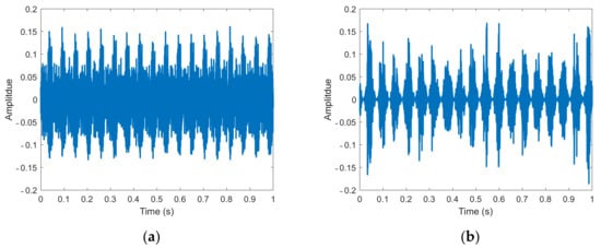
Figure 1.
Cyclo-stationary signal model: (a) deterministic part and (b) stochastic part.
Equations (8) and (9) are for the normal and defective signals composed of a combination of Equations (6) and (7), respectively. Equation (8) assumes that the signal can be measured in normal rotating machinery without the defective signal. It is the sum of the deterministic part shown in Equation (6) and white noise . Equation (9) is the sum of the deterministic part , the stochastic part , and white noise , assuming that the signal occurs in faulty rotating machinery.
Figure 2a shows the synthetic signal models of normal and defect expressed by Equations (8) and (9), respectively. It is difficult to distinguish between normal and defective signals in the time domain. However, comparing the spectrums in Figure 2b, the signal with defect shows a distinct difference in the band of 3.4 to 3.7 kHz compared to the normal signal. This band excited by the defect can be clearly differentiated by conducting envelope analysis according to the following method.

Figure 2.
Signal models for envelope analysis: (a) normal signal model (top) and faulty signal model (bottom); (b) spectrum of normal signal model (green) and spectrum of faulty signal model (black).
Figure 3a shows the filtered signals with aforementioned frequency band and envelopes of them. The top and bottom represent the normal signal model and the faulty signal model, respectively. When comparing the two, it can be seen that the faulty model shows a difference as much as the stochastic signal in Figure 1b.
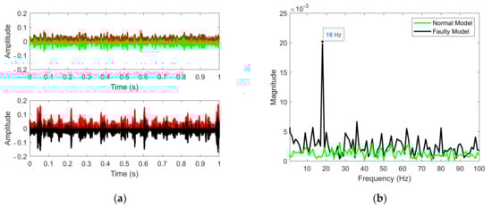
Figure 3.
Process of envelope analysis: (a) band-pass filtered signal models and envelope signals in time domain (top: normal signal model, bottom: faulty signal model); (b) envelope spectrum.
Figure 3b shows the spectrums obtained by Fourier transform on the two envelope signals, and are significantly different at the frequency corresponding to the period of the stochastic signal. In Figure 3b, a large magnitude means that the degree of envelope fluctuation and amplitude modulation are large. In other words, the signature of defect can be well observed. Therefore, the peak of the rotation frequency of the envelope spectrum can distinguish the faulty from the normal, and furthermore, it can be regarded as a feature to diagnose faults. In this study, threshold checking using these peak values is used to simply distinguish between normal and defective.
2.3. Degraded Detection Performance by Impulsive Noise
In the previous section, a general method of detecting defects through envelope analysis was introduced for cases in which rotating machinery has a periodic defective signal. However, various types of noise exist in an environment in which the fault detection of rotating machinery is implemented in practice. Unpredictable background noise causes the accuracy of envelope analysis to degrade. In particular, impulsive noise affects a wide frequency band, making it difficult to detect faults in envelope analysis. In the present study, we investigate the effect of impulsive noises on envelope analysis and propose an improvement method. Equations (10) and (11) represent the normal and defective signals in the presence of the impulsive noises . , given by Equation (12), is modeled as a rectangular wave with short time .
Figure 4 shows the normal model as a situation in which impulsive noise is contained at one time at 0.1 s. The signal to which the band-pass filter is applied and its envelope are shown in Figure 4a. Figure 4b shows the envelope spectrums. Compared to Figure 3b, which does not include the impulsive noise, the baseline of the spectrum is increased, and the peak of the spectrum due to the defective signal is less distinct. Figure 5 shows the envelope spectrums for the case where the impulsive noises are contained in four times. Red dotted line means the faulty signal without impulsive noise as the reference. Compared with Figure 4b, in which the impulsive noise is mixed in one time, it can be seen that the peak of the spectrum representing the defective signal is more difficult to distinguish from that of the normal signal. It is very hard to differentiate the peak magnitude of the defective signal without impulsive noise (red dotted line) and that of the normal signal with four impulsive noises (green line). This ambiguity occurs because not only the increase of the baseline by the impulsive noise, but also the periodicity of the impulsive noise is considered.
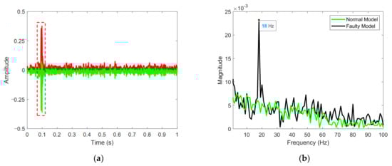
Figure 4.
(a) Filtered normal signal model with one impulsive noise at around 0.1 s. (b) Envelope spectrum of the normal and faulty model with one impulsive noise at around 0.1 s.
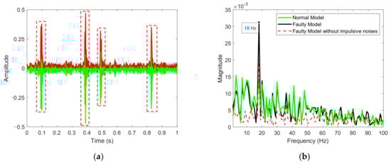
Figure 5.
Case where impulsive noises are contained four times at around 0.1, 0.4, 0.5, and 0.8 s. (a) Filtered normal signal and (b) envelope spectrum.
Impulsive noises are likely to be contained in several times in a short moment unless specific facilities such as anechoic chamber are installed for measurement. In this section, it has been confirmed that it is hard to distinguish between the normal and fault conditions when there are many impulsive noises where defects in rotating machinery are detected. In the next section, we propose a method to detect the signature of defect generated from rotating machinery even in the presence of such impulsive noises.
3. Improvement of Envelope Analysis
3.1. Time–Frequency Domain Approach for Envelope Analysis
In the previous section, the usefulness of envelope analysis was described in condition monitoring and fault detection related to the rotational speed of rotating machinery. In addition, the result of simulation showed that envelope analysis is no longer useful in cases contaminated by impulsive noises. In the present section, we propose a method that can utilize envelope analysis for defect detection even in the presence of intermittent impulsive noises. The method requires the transient signal analysis for the measured signals, unlike the analysis used in the previous section. In other words, a time–frequency analysis such as STFT or wavelet transform analysis should be used.
Time-frequency envelope analysis can also be performed by extracting the feature value of the envelope spectrum for a short-enough time and observing the change over the entire time of the measured data. Figure 6a shows STFT with a 0.33-s-length time window (both time resolution and frequency resolution are considered), which was the case applied to the envelope of the faulty model without impulsive noises shown in Figure 3b. Figure 6b shows the magnitude at the rotational frequency over time in the STFT shown in Figure 6a. Since the short time window is applied, there is a slight delay with the time axis. It is shown that the normal model and the faulty model are clearly distinguished.
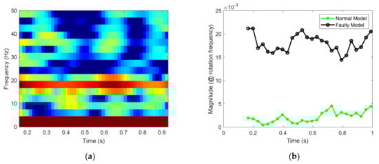
Figure 6.
Case without impulsive noise. (a) STFT of envelope of faulty signal model. (b) Magnitude at rotational frequency of 18 Hz over time with 0.33-s-length time window and 90% overlap.
Figure 7a shows the STFT for the faulty envelope with impulsive noise mixed in one time shown in Figure 4. The impulsive noise at around 0.1 s shown in Figure 4b has a large value in a wide frequency range from 0 to 0.25 s, and the time range is longer than the duration of impulsive noise because of the time window and overlap. Figure 7b shows the magnitude at the rotation frequency over time in the STFT shown in Figure 7a. Comparing the normal and faulty models, it is difficult to set a threshold to differentiate the normal model from the faulty model because the magnitude is larger in the 0 s to 0.25 s section due to the presence of impulsive noise at around 0.1 s.
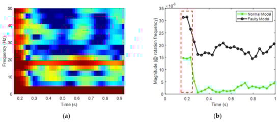
Figure 7.
Case where impulsive noise is contained one time at 0.1 seconds. (a) STFT of envelope of faulty signal model. (b) Magnitude at rotational frequency of 18 Hz over time with 0.33-s-length time window and 90% overlap.
Figure 8 shows a comparison of the peak value at the rotation frequency over time in the normal and faulty envelope spectrum when impulsive noises are mixed in four times, as shown in Figure 5. The area indicated by the red dotted square is the section affected by the impulsive noises. It can be seen that it is difficult to define a threshold for distinguishing between the normal model and faulty model in the entire time of measured signal. It is very contrasting with Figure 6b, which has no impulsive noise. Moreover, in practice, impulsive noises are not mixed in at the same time and the same magnitude for each measured signal. Therefore, we propose the method that can still detect defects through envelope analysis in the presence of impulsive noises as follows.
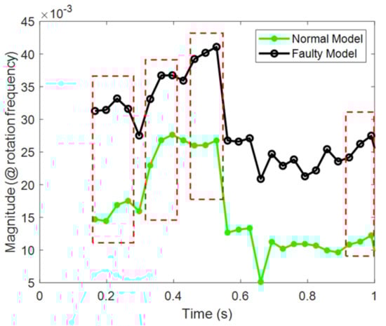
Figure 8.
Magnitude at rotational frequency of 18 Hz over time with 0.33-s-length time window and 90% overlap. Case where impulsive noises are contained four times at 0.1, 0.4, 0.5, and 0.8 s.
3.2. Methods for Overcoming Impulsive Noises
We investigated the phenomenon where the performance of defect detection through envelope analysis was degraded due to impulsive noise. Figure 9 shows the spectrum at 0.2 s in Figure 7a, which is contaminated by the large impulsive noise, and the spectrum at 0.7 s in Figure 7a, which is sufficiently out of the effect of the impulsive noise. In Figure 9a, the effect of impulsive noise compared to Figure 9b greatly increases the baseline of the spectrum, regardless of whether it is defective. As a result, the relative magnitude of the peak due to the defect is smaller than that in Figure 9b, making it difficult to set a threshold for defect detection.
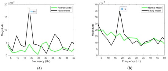
Figure 9.
Comparison of envelope spectrum (a) without an impulsive noise and (b) in the presence of an impulsive noise.
Defect detection through envelope analysis distinguishes between the normal and defect by using the magnitude at the rotational frequency of the rotating machinery, as described above. However, the magnitude of the impulsive noises in a wide frequency range that is irrelevant to rotation also affects the rotational frequency, making it difficult to detect defects. To overcome this disadvantageous phenomenon, we propose using the difference in magnitude at the rotation frequency and at frequencies sufficiently lower than the rotational frequency as a feature of defect detection. This idea is inspired by the frequency characteristics of very short time single rectangular wave given by Equations (12) and (13). is duration of impulsive noise and is the amplitude of . As gets shorter, appears as the horizontal stretched sinc function in frequency domain. Therefore, it can be seen that the magnitude of the relatively lower frequency is larger due to the short τ. This applies similarly to a single triangle wave.
The flowchart is shown in Figure 10. The window length is selected considering time resolution for impulsive noise and frequency resolution for rotating frequency. The time step is defined by the degree of overlap, window length , and total length of the measured signal. The window length should be selected as short as possible, but the frequency resolution , is reciprocal value of , sufficient to detect the rotational frequency must also be guaranteed. Then the magnitude is calculated from first time step to the end of time step . We can calculate the detection value at the end of the flowchart to define the threshold that can differentiate between normal and faulty.
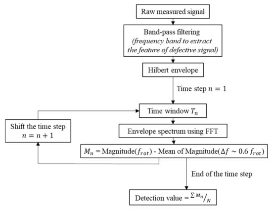
Figure 10.
Flowchart for proposed method.
The proposed method uses the characteristics of the impulsive rectangular signal, which has a very large instantaneous magnitude in the time domain but has broadly magnitudes from low to high frequencies in the frequency domain. In the spectrums with and without impulsive noise in Figure 9, in the normal signal, there is no difference between the magnitude at the rotational frequency of 18 Hz and the baseline magnitude of the lower frequencies in both. However, the defective signal shows the difference between the peak magnitude at the rotational frequency of 18 Hz and the baseline magnitude of the lower frequencies in both Figure 9a,b.
Figure 11 represents the cases of normal and defect depending on the number of impulsive noises contained. In the STFT of Figure 6a without impulsive noises, the difference between the magnitude at the rotational frequency of 18 Hz and the baseline magnitude of the lower frequencies is shown in Figure 11a. As shown in Figure 6b, which compares only the magnitude at the rotation frequency in the STFT, the normal and the defect in Figure 11a are clearly distinguished. Figure 11b shows the difference between the peak magnitude at the rotational frequency of 18 Hz and the baseline magnitude of the lower frequencies for the STFT in the presence of an impulsive noise shown in Figure 7a. In Figure 11, every normal case appears very close to zero or negative values. On the other hand, the defect has a much larger value, and even if much impulsive noises occur, the difference from the normal and the defect is still large. In the conventional method of detecting defects through envelope analysis, if the magnitude at the rotation frequency is larger than the threshold, it is judged as a defect. The method proposed in this study judges a defect if the difference between the magnitude at the rotational frequency and the baseline magnitude of the lower frequencies in the envelope spectrum is larger than the threshold.
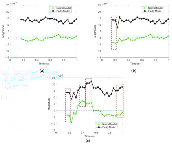
Figure 11.
The result of the proposed method to the signal models. The difference between the magnitude at rotational frequency and the baseline lower frequencies in short time envelope spectrum: (a) case without impulsive noises; (b) case in the presence of impulsive noise at 0.1 s; (c) case in the presence of four impulsive noises at 0.1, 0.4, 0.5, and 0.8 s.
4. Practical Example of the Proposed Method
The method proposed in this study was applied to the detection of noise-defects in an assembly line for ACs. The indoor AC unit is equipped with various types of fans to spread cold air in a room. However, if a problem occurs with constantly rotating fans or components around the fan, abnormal noise related to the rotation frequency of the fan is generated. The abnormal noise causes degradation of the product quality and consumer dissatisfaction. Therefore, companies that produce ACs have an inspection process to thoroughly sort out noise-defects before shipping out products.
In this process, noise-defects had been detected using the senses of workers. Recently, an automatic system has been developed to detect noise-defects by analyzing the noise signal measured near a product and has been installed in factories. However, in the site where noise is measured, there are various noises caused by random sources in other assembly processes, which make it difficult to detect defects effectively. Although an additional soundproof booth is installed to block out unpredictable noises from other processes, it not only can not completely block out the noises, but also increases the burden for cost and space. In particular, the impulsive noise caused by a conveyor belt moving products makes it more difficult to detect noise-defects.
Figure 12a shows the STFT of the acoustic signal of a normal AC measured for 5 s inside a soundproof booth where the product can enter and exit by a conveyor belt. The sounds from the back of ACs were measured for 5 s by fixed microphones while the ACs were moved at equal distance by the conveyor belt. The situation being measured was not controlled for testing, it was actually in production. In this figure, the impulsive noise seen at around 3 s (big white line circle) was investigated as noise caused by other technical processes. It was confirmed that the noise observed between 2 and 3 kHz and around 1 s (small white line circle) was introduced from the outside. Figure 12b shows the STFT of the acoustic signal of the AC investigated as a noise-defect caused by foreign substances hitting the blower fan. As the blower fan rotates, periodic noise is generated whenever it hits foreign substances. In order to automatically detect this noise-defect, the time–frequency envelope analysis method proposed in this study was applied.
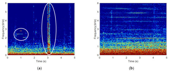
Figure 12.
Spectrogram of acoustic signals measured at near blower of air-conditioner (AC): (a) case of normal AC with impulsive noises and beep sounds; (b) case of faulty AC with abnormal noises.
A bandpass filter with cut-off frequencies of 3 and 6 kHz was applied to extract the signature of abnormal noises in conventional envelope spectrum. The bandwidth and center frequency of the filter were selected as the band representing the difference between normal and abnormal in frequency spectrum investigated in anechoic chamber conditions. At this time, frequencies of 2 to 3 kHz were not included in the band to exclude a beep sound that is not related to the noise-defect. Figure 13 shows the band-pass filtered time signal. Figure 13a,b shows the acoustic signals of the normal AC and the noise-defective AC, respectively. In the upper left of Figure 13a, the section between 0.5 and 1.5 s is enlarged and shown in the same scale as Figure 13b. Periodic impact signal, a feature of defective signal, is not observed. In Figure 13a, the impulsive noise is clearly visible at around 3 s, and no distinctive features appear in other time zones. On the other hand, in Figure 13b, the abnormal noise has the same period as the fan’s rotation speed and occurs in the form of impacts.
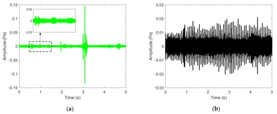
Figure 13.
Band-pass filtered acoustic signals: (a) normal AC with impulsive noises and beep sounds; (b) faulty AC with an abnormal noise.
Figure 14a compares the magnitude at the rotation frequency of around 13 Hz in the spectrum obtained with a 0.5-s-length time window (considering the time resolution and frequency resolution) and 50% overlap for the envelope of the normal and noise-defective signals shown in Figure 13. This figure shows only the magnitude at the rotational frequency according to the conventional method, and it is not possible to distinguish between the normal and the noise-defect signals due to impulsive noise at around 3 s. Figure 14b shows a graph considering the baseline magnitude of the low frequencies obtained by the method proposed in this study. The noise-defective signal shows almost no difference from Figure 14a, whereas the normal signal has a value close to zero overall. In particular, the value showed very dramatic improvement at around 3 s, at which the impulsive noise was mixed into the normal signal.
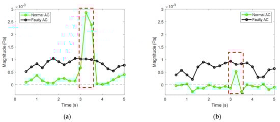
Figure 14.
Comparison of detection methods. (a) Conventional method using the peak value at the rotational frequency; (b) the proposed method using difference between the magnitude at the rotational frequency and the baseline magnitude of the lower frequencies.
To confirm the practicality of the proposed method, it was applied to 500 ACs that were under production. At this time, the detection rate was verified by also putting five ACs into the assembly line that had been investigated for noise-defects by the interference between foreign substances and the fans. Figure 15 shows the results of the proposed method for 500 normal ACs and the 5 noise-defective ACs for verification. The detection value used for the result is the mean of the values shown in Figure 14. Figure 15a shows the mean values obtained over time (0.5-s-length time window and 50% overlap) for only the magnitude of the rotation frequency in the envelope spectrum according to the conventional method. Figure 15b shows the difference between the magnitude at the rotational frequency and the baseline magnitude of the lower frequencies, which is the method proposed in this study. In Figure 15a, the five defects are not clearly distinguished from the 500 normal conditions. In comparison, Figure 15b shows the proposed method, and the 500 normal conditions and 5 defects are well distinguished.
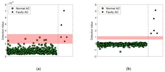
Figure 15.
Comparison of detection results: (a) conventional method; (b) the proposed method.
The practical application was verified by using acoustic signals measured in an assembly line producing ACs. The measured ACs were 500 normal units and 5 units with noise-defects. The detection performance was degraded because it was difficult to distinguish between the normal and the defects in the presence of impulsive noises using the conventional envelope analysis method. By eliminating the effects of the impulsive noises with the proposed method, the distinction between the normal and the defects became clear, and the detection performance was improved. However, the samples used in the real test for validation are 500 normal ACs and only 5 defective ACs caused by interference between the foreign materials and the fans. In the future, we will have to verify more defective ACs and various types of defects or other rotating machinery.
5. Conclusions
In this study, the simple time–frequency envelope analysis has been proposed to improve the degradation of the detection performance when impulsive noises contaminate the measured signals for condition monitoring and fault detection of the rotating machinery. When the impulsive noise is mixed in one time, the baseline of the envelope spectrum slightly increases, and the sharpness of the peak related to the defect becomes dull. When the impulsive noises are mixed in multiple times, the peaks related to the time interval between the impulsive noises can be observed to increase in the baseline of the envelope spectrum. This makes the sharpness of the peak indicating a defect that is very blurry and makes it impossible to distinguish between normal and defective signals.
Impulsive noise occurs for a very short time, so its effect can be eliminated by conducting envelope analysis on each section divided into several sections through a time window. The difference between the baseline magnitude was increased by the effect of the impulsive noise and the magnitude at the rotational frequency, which was used as an index for detecting defects. The improvement effect of the proposed method was verified through two methods: the simulation of a mathematically modeled signal and practical application to an assembly line that produces ACs.
For the simulation of synthetic signals, the models based on CS process representing typical properties of rotating machinery were used. Impulsive noise caused by unpredictable sources was modeled as single rectangular wave with short time. The proposed method was inspired by frequency characteristics of single rectangular wave in which the magnitude decreases as the frequency increases. The performance of the proposed method was verified by comparing to conventional method depending on the number of impulsive noises contained in the measured signal.
The real test in the assembly line producing ACs was implemented to verify the proposed method. The measured dataset using microphones consist of 500 normal ACs and 5 noise-defect ACs. The proposed method shows the ability to clearly differentiate the noise-defects from the normal even in the presence of impulsive noises, and contributes to the possibility of using a microphone, a non-invasive sensor, for fault detection. However, the samples used in the real test for validation are 500 normal ACs and only 5 defective ACs caused by interference between the foreign materials and the fans. In the future, we will have to verify more defective ACs and various types of defects or other rotating machinery. Moreover, the approaches of big data and deep learning will be required for the development of the PHM framework.
Author Contributions
Conceptualization, D.-H.L.; methodology, W.-B.J. and S.A.; formal analysis, C.H.; writing—original draft preparation, D.-H.L.; writing—review and editing, S.A.; visualization, S.A.; supervision, W.-B.J.; project administration, C.H. and W.-B.J.; All authors have read and agreed to the published version of the manuscript.
Funding
This research was supported by Basic Science Research Program through the National Research Foundation of Korea (NRF) funded by the Ministry of Education (NRF-2020R1I1A3064576).
Institutional Review Board Statement
Not applicable.
Informed Consent Statement
Not applicable.
Data Availability Statement
Not applicable.
Conflicts of Interest
The authors declare no conflict of interest.
References
- Venkatasubramanian, V.; Rengaswamy, R.; Yin, K.; Kavuri, S.N. A review of process fault detection and diagnosis part I: Quantitative model-based methods. Comput. Chem. Eng. 2003, 27, 293–311. [Google Scholar] [CrossRef]
- Sharma, S.; Tiwari, S.K. Sukhjeet Singh Integrated approach based on flexible analytical wavelet transform and permutation entropy for fault detection in rotary machines. Measurement 2021, 169, 108389. [Google Scholar] [CrossRef]
- Kim, J.H. Fault detection for manufacturing home air conditioners using wavelet transform. Int. J. Precis. Eng. Manuf. 2016, 17, 1299–1303. [Google Scholar] [CrossRef]
- Kim, J.H. Time Frequency Image and Artificial Neural Network Based Classification of Impact Noise for Machine Fault Diagnosis. Int. J. Precis. Eng. Manuf. 2018, 19, 821–827. [Google Scholar] [CrossRef]
- Henriquez, P.; Alonso, J.B.; Ferrer, M.A.; Travieso, C.M. Review of Automatic Fault Diagnosis Systems Using Audio and Vibration Signals. IEEE Trans. Syst. Man Cybern. Syst. 2014, 44, 642–652. [Google Scholar] [CrossRef]
- Bin, G.F.; Gao, J.J.; Li, X.J.; Dhillon, B.S. Early fault diagnosis of rotating machinery based on wavelet packets-Empirical mode decomposition feature extraction and neural network. Mech. Syst. Signal Process. 2012, 27, 696–711. [Google Scholar] [CrossRef]
- Antoni, J.; Bonnardot, F.; Raad, A.; El Badaoui, M. Cyclostationary modelling of rotating machine vibration signals. Mech. Syst. Signal Process. 2004, 18, 1285–1314. [Google Scholar] [CrossRef]
- Tang, G.; Pang, B.; Tian, T.; Zhou, C. Fault diagnosis of rolling bearings based on improved fast spectral correlation and optimized random forest. Appl. Sci. 2018, 8, 1859. [Google Scholar] [CrossRef]
- Klausen, A.; Robbersmyr, K.G.; Karimi, H.R. Autonomous Bearing Fault Diagnosis Method based on Envelope Spectrum. IFAC-PapersOnLine 2017, 50, 13378–13383. [Google Scholar] [CrossRef]
- Vicuña, C.M.; Acuña, D.Q. Cyclostationary Processing of Vibration and Acoustic Emissions for Machine Failure Diagnosis. In Cyclostationarity: Theory and Methods; Chaari, F., Leśkow, J., Napolitano, A., Sanchez-Ramirez, A., Eds.; Lecture Notes in Mechanical Engineering; Springer International Publishing: Cham, Germany, 2014; pp. 141–156. ISBN 978-3-319-04186-5. [Google Scholar]
- Abboud, D.; Antoni, J.; Sieg-Zieba, S.; Eltabach, M. Envelope analysis of rotating machine vibrations in variable speed conditions: A comprehensive treatment. Mech. Syst. Signal Process. 2017, 84, 200–226. [Google Scholar] [CrossRef]
- Barszcz, T.; Jabłoński, A. A novel method for the optimal band selection for vibration signal demodulation and comparison with the Kurtogram. Mech. Syst. Signal Process. 2011, 25, 431–451. [Google Scholar] [CrossRef]
- Zhao, X.; Qin, Y.; He, C.; Jia, L.; Kou, L. Rolling element bearing fault diagnosis under impulsive noise environment based on cyclic correntropy spectrum. Entropy 2019, 21, 50. [Google Scholar] [CrossRef] [PubMed]
- Antoni, J. The infogram: Entropic evidence of the signature of repetitive transients. Mech. Syst. Signal Process. 2016, 74, 73–94. [Google Scholar] [CrossRef]
- Mosleh, A.; Montenegro, P.A.; Costa, P.A.; Calçada, R. Railway Vehicle Wheel Flat Detection with Multiple Records Using Spectral Kurtosis Analysis. Appl. Sci. 2021, 11, 4002. [Google Scholar] [CrossRef]
- Mosleh, A.; Montenegro, P.; Alves Costa, P.; Calçada, R. An approach for wheel flat detection of railway train wheels using envelope spectrum analysis. Struct. Infrastruct. Eng. 2020, 1–20. [Google Scholar] [CrossRef]
- Smith, W.A.; Fan, Z.; Peng, Z.; Li, H.; Randall, R.B. Optimised Spectral Kurtosis for bearing diagnostics under electromagnetic interference. Mech. Syst. Signal Process. 2016, 75, 371–394. [Google Scholar] [CrossRef]
- Miao, Y.; Zhao, M.; Lin, J. Improvement of kurtosis-guided-grams via Gini index for bearing fault feature identification. Meas. Sci. Technol. 2017, 28. [Google Scholar] [CrossRef]
- Tyagi, S.; Panigrahi, S.K. An improved envelope detection method using particle swarm optimisation for rolling element bearing fault diagnosis. J. Comput. Des. Eng. 2017, 4, 305–317. [Google Scholar] [CrossRef]
- Elasha, F.; Greaves, M.; Mba, D. Planetary bearing defect detection in a commercial helicopter main gearbox with vibration and acoustic emission. Struct. Health Monit. 2018, 17, 1192–1212. [Google Scholar] [CrossRef]
- Peeters, C.; Guillaume, P.; Helsen, J. Vibration-based bearing fault detection for operations and maintenance cost reduction in wind energy. Renew. Energy 2018, 116, 74–87. [Google Scholar] [CrossRef]
- Randall, R.B.; Antoni, J. Rolling element bearing diagnostics—A tutorial. Mech. Syst. Signal Process. 2011, 25, 485–520. [Google Scholar] [CrossRef]
- Maiz, S.; El Badaoui, M.; Bonnardot, F.; Dudek, A.; Leskow, J. Deterministic/cyclostationary signal separation using bootstrap. IFAC Proc. Vol. 2013, 46, 641–646. [Google Scholar] [CrossRef]
- Abboud, D.; Antoni, J.; Sieg-Zieba, S.; Eltabach, M. Deterministic-random separation in nonstationary regime. J. Sound Vib. 2016, 362, 305–326. [Google Scholar] [CrossRef]
- Wodecki, J.; Michalak, A.; Zimroz, R. Local damage detection based on vibration data analysis in the presence of Gaussian and heavy-tailed impulsive noise. Meas. J. Int. Meas. Confed. 2021, 169, 108400. [Google Scholar] [CrossRef]
- Vilela, R.M.; Metrôlho, J.C.; Cardoso, J.C. Machine and industrial monitorization system by analysis of acoustic signatures. In Proceedings of the 12th IEEE Mediterranean Electrotechnical Conference (IEEE Cat. No.04CH37521), Dubrovnik, Croatia, 12–15 May 2004; Volume 1, pp. 277–279. [Google Scholar]
- Liu, T.; Qiu, T.; Luan, S. Cyclic Correntropy: Foundations and Theories. IEEE Access 2018, 6, 34659–34669. [Google Scholar] [CrossRef]
- Luan, S.; Qiu, T.; Zhu, Y.; Yu, L. Cyclic correntropy and its spectrum in frequency estimation in the presence of impulsive noise. Signal Process. 2016, 120, 503–508. [Google Scholar] [CrossRef]
- Baek, W.; Kim, D.Y. In-Process Noise Detection System for Product Inspection by Using Acoustic Data. IFIP Adv. Inf. Commun. Technol. 2019, 567, 413–420. [Google Scholar] [CrossRef]
- Saucedo-Espinosa, M.A.; Escalante, H.J.; Berrones, A. Detection of defective embedded bearings by sound analysis: A machine learning approach. J. Intell. Manuf. 2017, 28, 489–500. [Google Scholar] [CrossRef]
- Leclère, Q.; Pruvost, L.; Parizet, E. Angular and temporal determinism of rotating machine signals: The diesel engine case. Mech. Syst. Signal Process. 2010, 24, 2012–2020. [Google Scholar] [CrossRef][Green Version]
- He, Q.; Ding, X. Structural Health Monitoring; Yan, R., Chen, X., Mukhopadhyay, S.C., Eds.; Smart Sensors, Measurement and Instrumentation; Springer International Publishing: Cham, Germany, 2017; Volume 26, ISBN 978-3-319-56125-7. [Google Scholar]
- He, Q.; Wang, X.; Zhou, Q. Vibration sensor data denoising using a time-frequency manifold for machinery fault diagnosis. Sensors 2013, 14, 382–402. [Google Scholar] [CrossRef] [PubMed]
- Amini, A.; Entezami, M.; Huang, Z.; Rowshandel, H.; Papaelias, M. Wayside detection of faults in railway axle bearings using time spectral kurtosis analysis on high-frequency acoustic emission signals. Adv. Mech. Eng. 2016, 8, 1–9. [Google Scholar] [CrossRef]
- Islam, M.M.M.; Kim, J.M. Time–frequency envelope analysis-based sub-band selection and probabilistic support vector machines for multi-fault diagnosis of low-speed bearings. J. Ambient Intell. Humaniz. Comput. 2017, 1–16. [Google Scholar] [CrossRef]
- Kumar, A.; Kumar, R. Time-frequency analysis and support vector machine in automatic detection of defect from vibration signal of centrifugal pump. Meas. J. Int. Meas. Confed. 2017, 108, 119–133. [Google Scholar] [CrossRef]
- Petrillo, A.; Picariello, A.; Santini, S.; Scarciello, B.; Sperlí, G. Model-based vehicular prognostics framework using Big Data architecture. Comput. Ind. 2020, 115. [Google Scholar] [CrossRef]
- Manco, G.; Ritacco, E.; Rullo, P.; Gallucci, L.; Astill, W.; Kimber, D.; Antonelli, M. Fault detection and explanation through big data analysis on sensor streams. Expert Syst. Appl. 2017, 87, 141–156. [Google Scholar] [CrossRef]
- Jing, L.; Zhao, M.; Li, P.; Xu, X. A convolutional neural network based feature learning and fault diagnosis method for the condition monitoring of gearbox. Meas. J. Int. Meas. Confed. 2017, 111, 1–10. [Google Scholar] [CrossRef]
- De santo, A.; Galli, A.; Gravina, M.; Moscato, V.; Sperli, G. Deep Learning for HDD health assessment: An application based on LSTM. IEEE Trans. Comput. 2020, 1–12. [Google Scholar] [CrossRef]
- Feldman, M. Hilbert transform in vibration analysis. Mech. Syst. Signal Process. 2011, 25, 735–802. [Google Scholar] [CrossRef]
- Antoni, J. Cyclostationarity by examples. Mech. Syst. Signal Process. 2009, 23, 987–1036. [Google Scholar] [CrossRef]
- Gardner, W.; Franks, L. Characterization of cyclostationary random signal processes. IEEE Trans. Inf. Theory 1975, 21, 4–14. [Google Scholar] [CrossRef]


Publisher’s Note: MDPI stays neutral with regard to jurisdictional claims in published maps and institutional affiliations. |
© 2021 by the authors. Licensee MDPI, Basel, Switzerland. This article is an open access article distributed under the terms and conditions of the Creative Commons Attribution (CC BY) license (https://creativecommons.org/licenses/by/4.0/).