Abstract
The estimation of variables that are normally not measured or are unmeasurable could improve control and condition monitoring of wind turbines. A cost-effective estimation method that exploits machine learning is introduced in this paper. The proposed method allows a potentially expensive sensor, for example, a LiDAR sensor, to be shared between multiple turbines in a cluster. One turbine in a cluster is equipped with a sensor and the remaining turbines are equipped with a nonlinear estimator that acts as a sensor, which significantly reduces the cost of sensors. The turbine with a sensor is used to train the estimator, which is based on an artificial neural network. The proposed method could be used to train the estimator to estimate various different variables; however, this study focuses on wind speed and aerodynamic torque. A new controller is also introduced that uses aerodynamic torque estimated by the neural network-based estimator and is compared with the original controller, which uses aerodynamic torque estimated by a conventional aerodynamic torque estimator, demonstrating improved results.
1. Introduction
Operation and maintenance (O&M) costs account for a significant proportion of the total annual costs of a wind turbine. Typically, O&M costs account for more than 20% of the total levelised cost per kWh. Therefore, in recent years, reducing O&M costs, which include control and condition monitoring, has become even more important in wind turbine and farm operational strategies because it has a long-lasting impact on the profitability and efficiency of wind site operations.
Providing cost-effective access to various different variables in wind turbines and farms could help to reduce O&M costs by improving control and condition monitoring capabilities. Allowing access to variables that are normally not measured could, in fact, increase the costs because additional potentially expensive sensors might need to be introduced. However, the proposed approach is cost effective as it only requires a single sensor between multiple turbines. More precisely, it is proposed that one sensor be shared between multiple turbines (five in this paper), that is, one turbine is equipped with a potentially expensive sensor and each of the remaining turbines (four in this paper) is equipped with an estimator. Each estimator is based on a neural network (NN) [1,2]. Note that it is often not feasible to exploit more conventional estimators, such as observers [3,4] including extended Kalman filters [5,6], since the behaviour of a wind turbine is highly nonlinear, and designing such observers would require a highly sophisticated mathematical model. Therefore, an NN is adopted to design nonlinear estimators that could replace sensors.
The proposed method could be adopted for estimating various different useful variables; however, this study focuses on two variables: wind speed and aerodynamic torque. Wind speed and aerodynamic torque estimated by the NN-based estimators are compared with those estimated by conventional wind speed and aerodynamic torque estimators, respectively.
Many existing wind turbine controllers require the estimation of aerodynamic torque, which is normally conducted by conventional aerodynamic torque estimators, such as the one introduced in [7]. In this paper, a new controller is introduced that uses aerodynamic torque estimated by the NN-based estimator and is compared with the original controller, which uses aerodynamic torque estimated by the conventional aerodynamic torque estimator, demonstrating improved results. Wind speed estimated by the proposed NN-based estimator could also help to improve wind turbine control; however, that is not discussed in this paper.
Most estimation-related work in the wind turbine control community deals with wind speed estimation, such as the work presented in [8,9,10]. A detailed survey on this topic is presented in [11]. The NN-based method proposed in this paper is novel, as no other existing work realises wind speed estimation at a wind farm level taking into account the associated costs. Modern control topics currently of interest in the wind turbine control community include improving the control performance by incorporating wind speed (normally measured using a LiDAR) into the controller design, such as in [12,13,14,15]. However, the estimation method proposed here allows the use of not only wind speed but also other useful variables that are normally not measured as part of the controller design. As an example, the second part of this paper demonstrates potential improvement of the control performance, which can be achieved by improving the accuracy of aerodynamic torque estimation.
In summary, the primary contributions of this paper are the development of NN-based estimators (focusing on the estimation of wind speed and aerodynamic torque here) and the improvement of the wind turbine controller realised by incorporating the improved estimation of aerodynamic torque in the original controller design.
The stall-regulated version [16] of the exemplar 5 MW wind turbine model of the Supergen Wind Hub in Matlab/Simulink© [7], which has been used for various UK and EU projects over the past 12 years, is employed here to simulate wind turbines and farms.
The remainder of this paper is organised as follows: The model and controller, as well as the wind speed model required to run the model, are described in Section 2. The proposed NN-based nonlinear estimation method and simulation results are presented in Section 3. In Section 4, a controller that uses aerodynamic torque estimated by the NN-based estimator is introduced and compared with the original controller that uses aerodynamic torque estimated by the conventional aerodynamic torque estimator. Conclusions and suggestions for future work are provided in Section 5.
2. Wind Turbine and Wind Speed Modelling and Wind Turbine Control
The wind turbine model used in this study is the stall-regulated version of the Supergen 5 MW exemplar turbine, which was developed as part of the collective control strategy introduced in [16]. The wind turbine model, corresponding to the block labelled “turbine” in Figure 1 and mainly consisting of modules or sub-models of rotor and aerodynamics, drive-train and induction generator, is presented in this section. The wind speed model required to simulate the wind turbine model and the full envelope wind turbine controller based on Model Predictive Control (MPC) [17,18], corresponding to the block labelled “controller” in Figure 1, are also presented in this section.
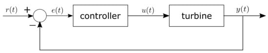
Figure 1.
Common control scheme.
2.1. Wind Speed
The point wind speeds (as measured by an anemometer) across the cluster of five turbines, which consider the flow dynamics across the turbines, the interactions between the turbines and the flow fields, including the wakes and turbulence, are obtained using Bladed, a high-fidelity aeroelastic model by DNV. (Rotor) effective wind speed, defined as the spatially-averaged wind speeds across the rotor plane [19] experienced by the wind turbine, is obtained by filtering the point wind speed through the wind speed model introduced in [20]. The resulting effective wind speeds used to simulate the wind turbine in this paper are shown in Figure 2. Note that effective wind speeds are only shown for a mean wind speed of 14 m/s because they exhibit very close trends at other mean wind speeds.
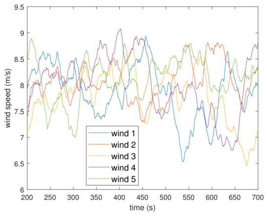
Figure 2.
Effective wind speeds for turbines 1 to 5.
2.2. Rotor and Aerodynamics
The rotor and aerodynamics module is described by the following equation:
where is the aerodynamic or hub torque, is the air density, R is the rotor radius, V is the effective wind speed (Section 2.1) and is the power coefficient unique to the rotor design. is the tip-speed ratio given by
where is the rotor speed.
2.3. Drive-Train Dynamics
The drive-train dynamics are described by the following equation [7]:
where is rotor speed, is generator speed, is aerodynamic torque and is generator torque. Neglecting the intermediate to high frequency components, , , , and all reduce to
where is the high speed shaft external damping coefficient in (Nm/rad/s), is the low-speed shaft external damping coefficient (in Nm/rad/s), is the rotor inertia (in kg m), is the generator inertia (in m) and N is the gearbox ratio.
2.4. Induction Generator Dynamics
In the turbine adopted here, the standard synchronous generator of the original Supergen 5MW exemplar turbine [7] has been replaced by an induction generator to increase the damping. The resulting model is described by the following equation:
where and represent the power grid frequency and the number of poles, respectively.
2.5. Full Envelope Control
Wind turbine control normally consists of two components: control synthesis (including control regulation in each operating mode) and determination of the operating strategy in the speed-torque plane (such as the one shown in Figure 3). The former is related to designing a linear controller in each mode and the latter includes switching smoothly at appropriate wind speeds between different modes. Here, MPC is selected as the control algorithm; however, others, such as linear quadratic Gaussian and H controllers, are equally pertinent. As shown in Figure 3, in modes 1 and 3, which could be considered buffering zones, constant speeds are maintained. In mode 2, the curve is tracked to extract as much energy as possible from the wind and, in mode 4, the wind turbine stalls to maintain the rated power in high wind speeds. The green curves represent wind speeds increasing from 4 to 24 m/s with an increment of 0.5 m/s. Detailed information about wind turbine controllers is available in the literature [19,21].
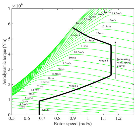
Figure 3.
Control strategy in the speed-torque plane; the green curves represent wind speeds increasing from 4 to 24 m/s with an increment of 0.5 m/s.
The frequency of each mini-grid can be adjusted via a centralised AC–DC–AC power converter, allowing a variable-speed control strategy, as opposed to the constant-speed control strategy, to be adopted here even though the turbines are constant speed machines. Further details on the type of wind turbines adopted here can be found in the literature [16].
3. Neural Network Based Estimators
Having access to certain variables that are typically not measured could improve the control and condition monitoring of wind turbines; however, this would require potentially expensive sensors for each turbine. To solve this problem, we propose that only a single turbine in a wind farm of multiple turbines (five in this paper) be equipped with a potentially expensive sensor. Each remaining turbine could be equipped with a nonlinear estimator based on an NN, which would essentially replace the expensive sensor as illustrated in Figure 4. This scheme could be used to estimate various variables in a cost-effective manner; however, this paper only considers two variables, that is, wind speed and aerodynamic torque.
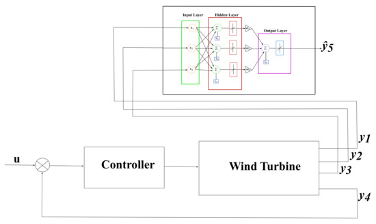
Figure 4.
NN-based estimator.
The NN structure used in this paper, and the full procedure for designing and training the NN-based estimators for wind speed and torque estimation, are given in Section 3.2. The estimation results of the NN-based estimators are compared to those of conventional mathematical torque and wind speed estimators in Section 3.3.
3.1. Existing Estimators
3.1.1. Wind Speed Estimation
The wind speed estimator introduced here is based on Equation (1). Note that both sides of Equation (1) are divided by , yielding
Note that the wind speed is given by the following equation:
Equation (6) can be expressed for as follows:
where denotes rotor speed. Table can be updated to . Here, and are known; thus, can be derived. Then, the wind speed V can be estimated using Equation (7).
This is a commonly used wind speed estimator [22], and the estimation results of the proposed NN-based wind speed estimator (Section 3.2) are compared to those of this wind speed estimator (Equation (8)) in this section.
3.1.2. Torque Estimation
Typically, aerodynamic torque is estimated (rather than measured) using an estimator that uses generator torque measurements as follows:
where denotes the aerodynamic torque estimate, N is the gearbox ratio, is the rotor inertia, is the generator inertia, is the low-speed shaft damping coefficient, is the high-speed shaft damping coefficient and H is the hub speed.
This is a common aerodynamic torque estimator [7], and the estimation results of the proposed NN-based torque estimator (Section 3.2) are compared to those of this torque estimator (Equation (9)) in this section.
3.2. NN-Based Estimators
An NN can be described as a model with a layered structure that resembles the human brain, including layers of connected nodes [23]. NNs are inspired by how the human brain works and can include many processing layers with simple elements running in parallel. Typically, an NN contains an input layer, one or more hidden layers and an output layer (Figure 5). The layers are combined through neurons or nodes, and the output of each layer becomes the input to the next layers. Recently, NNs have been applied to various tasks. In this study, we employ an NN as a pattern recognition method to identify a highly nonlinear model.
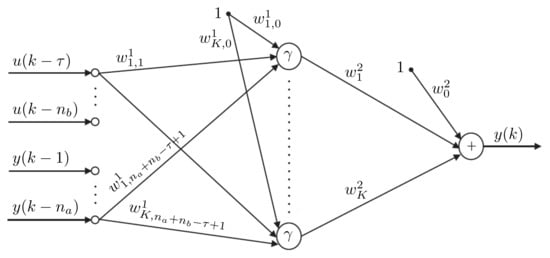
Figure 5.
Structure of DLP feedforward NN.
The double-layer perceptron (DLP) feedforward NN shown in Figure 5 is adopted in this study. Although many different types of NN are available, the DLP feedforward structure is one of the most popular structures. The NN structure in the figure describes the following generic nonlinear model [24]:
where is the time delay, and correspond to the order of the model, and the nonlinear function represents the nonlinear model. This NN includes inputs, a single output , K nonlinear hidden nodes represented by , and a single linear output element (corresponding to the sum block shown in Figure 5). In addition, the following bipolar sigmoid transfer function is used in this network:
where parameter is typically set to 1.
The weights of the first layer are denoted by , where , and the weights of the second layer are denoted by , where . The output signal is expressed as follows [25]:
where the sum of input signals of the hidden node is
Subsequently, the NN is trained by minimising the following index:
where is the output of the NN, and denotes the output measurements used to train the NN. Here, the Levenberg–Marquardt [26] algorithm, also referred to as the damped least-squares method, is employed as the nonlinear gradient optimisation algorithm. It uses the Jacobian for calculations, which assumes that the performance is a mean or sum of squared errors. For training the NN, data sets are broken down into three: 70% for training, 20% for testing and 10% for validation. Readers are referred to the literature [1,2,24] for additional details.
The procedure used to design an NN-based estimator is summarised as follows:
- Turbine 1 (out of five in this paper) is equipped with a sensor, and each remaining turbine (i.e., Turbines 2 to 5) is equipped with a nonlinear NN-based estimator, as shown in Figure 4.
- The inputs and outputs are measured and collected from Turbine 1 using the single sensor at regular intervals, that is, every 1000 s. Note that the output could be different variables but is limited to wind speed or aerodynamic torque in this paper. To estimate the aerodynamic torque, the inputs are a combination of generator torque, generator speed, fore-aft acceleration (FAA) and tower bending moment (TBM). The output is aerodynamic torque; therefore, a sensor is required to measure aerodynamic torque. To estimate the wind speed, the inputs are a combination of generator torque, TBM and FAA, and the output is wind speed. Therefore, a sensor (i.e., LiDAR) is required to measure the wind speed. Note that different combinations of generator torque, generator speed, TBM and FAA are tested.
- Based on these measurements, the nonlinear estimator shown in Figure 4 is designed and trained appropriately using the NN described in this section.
- Each remaining turbine is equipped with the trained estimator, which estimates the wind speed or aerodynamic torque.
- Steps 2, 3 and 4 are repeated every 1000 s.
Note that, for the purpose of improving the control performance, highly accurate measurement of the upcoming wind speed is required, which can only be achieved through the use of a LiDAR. Note that anemometers cannot provide such accurate measurements and are normally used for yawing and starting up/shutting down the wind turbines, which do not require highly accurate measurements. However, the main drawback of using a LiDAR is the cost, and we attempt to tackle the problem by proposing a cost-effective estimation method that allows a number of turbines to share a single LiDAR.
The Matlab/SIMULINK model of the Supergen 5 MW exemplar turbine (stall-regulated version), described in Section 2, is used to simulate each turbine and provide the data required to train the NN-based estimators. In addition, the wind speeds given in Section 2.1 are used to simulate appropriately correlated wind speeds. As described in Step 2, the following combinations or scenarios are considered to train the NN estimator to estimate aerodynamic torque.
- Scenario 1: rotor speed, generator speed and TBM.
- Scenario 2: generator torque, generator speed and TBM.
- Scenario 3: fore-aft acceleration, rotor speed and TBM.
The following combinations or scenarios are considered for training the NN-based estimator to estimate wind speed.
- Scenario 4: generator torque, rotor speed and TBM.
- Scenario 5: rotor speed, fore-aft acceleration and TBM.
3.3. Estimation Results
3.3.1. Aerodynamic Torque
Figure 6 and Figure 7 show, in black, the aerodynamic torque estimated using the NN-based estimator for Scenario 1 in both the time (left column) and frequency (right column) domains, compared to that estimated using the conventional aerodynamic torque estimator (Section 3.1) (in blue) and the actual measurements (in red). Figure 6 and Figure 7 show the results for Turbines 1 and 5, respectively, which were selected randomly because Turbines 2 to 4 produce similar results. In real world scenarios, the measurements would only be available from Turbine 1 (i.e., the turbine with the sensor); however, the measurements from Turbine 5 are also included for comparison purposes. Note that this also applies to Figure 8 and Figure 9 for Scenario 2 and Figure 10 and Figure 11 for Scenario 3 in the following:
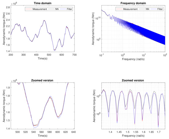
Figure 6.
Scenario 1: Aerodynamic torque estimation from Turbine 1.
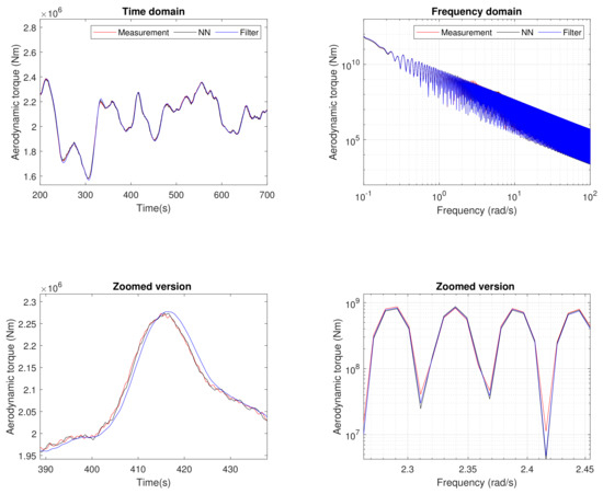
Figure 7.
Scenario 1: Aerodynamic torque estimation from Turbine 5.

Figure 8.
Scenario 2: Aerodynamic torque estimation from Turbine 1.
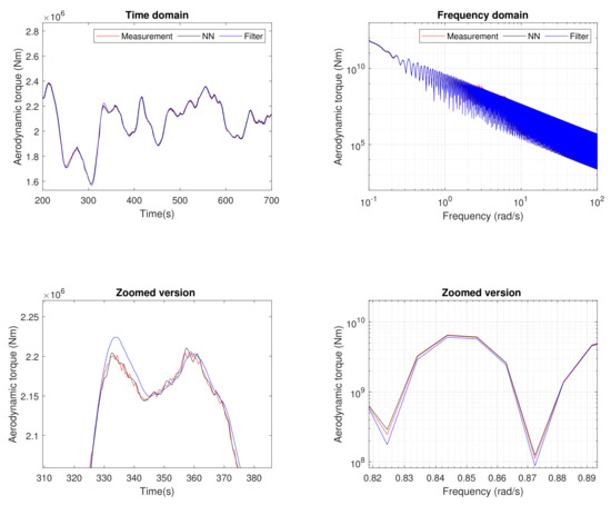
Figure 9.
Scenario 2: Aerodynamic torque estimation from Turbine 5.
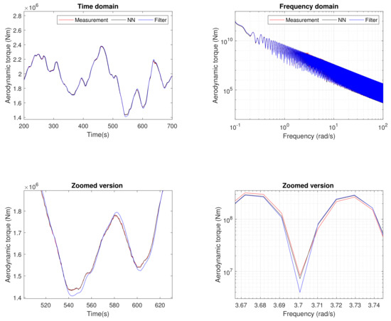
Figure 10.
Scenario 3: Aerodynamic torque estimation from Turbine 1.

Figure 11.
Scenario 3: Aerodynamic torque estimation from Turbine 5.
In Scenario 1, for both turbines, the time domain results demonstrate that the aerodynamic torque estimated by the NN-based estimator tracks the measurements more closely than that estimated by the conventional aerodynamic torque estimator; however, the improvement shown by the corresponding power spectra is not as significant.
For Scenario 2, Figure 8 and Figure 9 demonstrate similar results to those observed in Scenario 1 in the time-domain, that is, for both turbines, the aerodynamic torque estimated by the NN-based estimator tracks the measurements more closely than that estimated by the conventional aerodynamic torque estimator. The corresponding power spectra shown in Figure 8 and Figure 9 illustrate that the aerodynamic torque estimated by the NN-based estimator tracks the measurements more closely than that estimated by the conventional aerodynamic torque estimator in the frequency domain. The power spectra also exhibit improved results compared to those of Scenario 1, which implies that the combination of variables used to train the NN in Scenario 2 is better than the combination used in Scenario 1.
For Scenario 3, Figure 10 and Figure 11 show similar results to those obtained for Scenarios 1 and 2 in the time domain, that is, for both turbines, the aerodynamic torque estimated by the NN-based estimator tracks the measurements more closely than that estimated by the conventional aerodynamic torque estimator in the time domain. The corresponding power spectra shown in Figure 8 and Figure 9 demonstrate that the aerodynamic torque estimated by the NN-based estimator tracks the measurements more closely than that estimated by the conventional aerodynamic torque estimator in the frequency domain. In addition, the corresponding power spectra illustrate more improved results than those obtained in Scenarios 1 and 2, which indicates that the combination of variables used to train the NN in Scenario 3 is better than the combinations of variables used in Scenarios 1 and 2.
In summary, the NN-based estimator performs best in Scenario 3 (of Scenarios 1 to 3); that is, when fore-aft acceleration, rotor speed and TBM are used as the inputs to train the NN. The NN-based estimator outperforms the conventional aerodynamic torque estimator in each scenario, which could be due to the fact that the conventional aerodynamic torque estimator includes a low-pass filter as described by Equation (9), which is required to ensure that the estimator is practically feasible.
3.3.2. Wind Speed
Figure 12 and Figure 13 show (in black) the wind speed estimated by the NN-based estimator for Scenario 4 in both the time (left column) and frequency (right column) domains compared to that estimated by the conventional wind speed estimator (Section 3.1) (in blue) and the actual measurements (in red). Figure 12 and Figure 13 are for Turbines 1 and 5, respectively, and were selected randomly because Turbines 2 to 4 produced similar results. In real world scenarios, the measurements would only be available from Turbine 1, that is, the turbine with a LiDAR system; however, the measurements from Turbine 5 are included for comparison purposes. Note that this applies to Figure 12 and Figure 13 for Scenario 4 and Figure 14 and Figure 15 for Scenario 5.
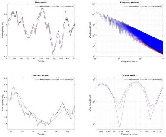
Figure 12.
Scenario 4: Wind speed estimation from Turbine 1.
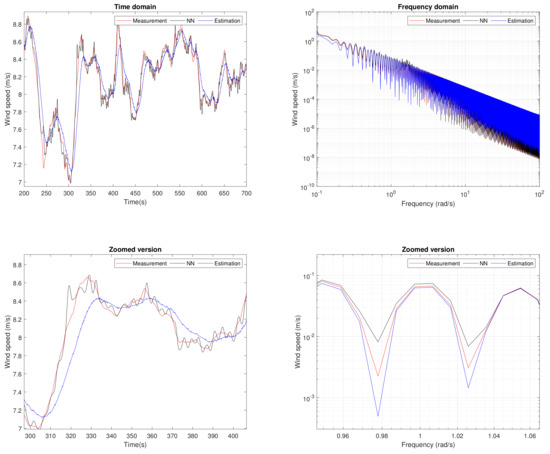
Figure 13.
Scenario 4: Wind speed estimation from Turbine 5.
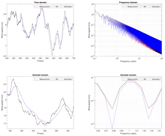
Figure 14.
Scenario 5: Wind speed estimation from Turbine 1.
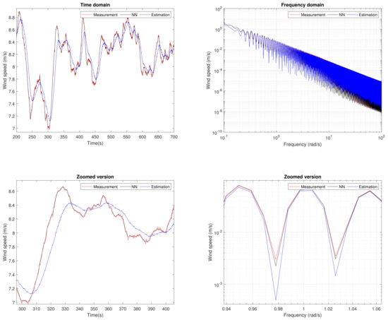
Figure 15.
Scenario 5: Wind speed estimation from Turbine 5.
In Scenario 4, for both turbines, the time and frequency results demonstrate that the wind speed estimated by the NN-based estimator tracks the measurements more closely than that estimated by the conventional wind speed estimator. For Scenario 5, Figure 14 and Figure 15 demonstrate that the wind speed estimated by the NN-based estimator tracks the measurements more closely than that estimated by the conventional wind speed estimator for both turbines in the time and frequency domains. Both the time plots and power spectra also clearly demonstrate improved results compared to those obtained in Scenario 4, which indicates that the combination of variables used to train the NN in Scenario 5 is better than that used in Scenario 4.
In summary, the NN-based estimator performs best in Scenario 5 (between Scenarios 4 and 5), that is, when rotor speed, fore-aft acceleration and TBM are used as the inputs for training the NN. The NN-based estimator outperforms the conventional wind speed estimator in each scenario, which is partly due to the limited accuracy of the conventional wind speed estimator model.
4. Control Using Improved Aerodynamic Torque Estimation
As shown in Figure 3 (Section 2.5), constant speeds are maintained in modes 1 and 3, which are buffering zones; the curve is tracked to extract as much energy as possible from the wind in mode 2; and the wind turbine stalls to maintain the rated power in high wind speeds in mode 4.
The grid frequency, and thus the rotor speed, vary in response to the aerodynamic torque such that the operating strategy curve (Figure 3 and Figure 16) is tracked. Generally, aerodynamic torque is estimated (rather than measured) by the conventional aerodynamic torque estimator (Section 3) from the measured generator torque. In Section 3, the simulation results demonstrate that the aerodynamic torque estimation is improved using the NN-based estimator. Here, a new controller that uses aerodynamic torque estimated by the NN-based estimator (Section 4) is presented and compared to the original controller that uses aerodynamic torque estimated by the conventional aerodynamic torque estimator (Section 3.2).
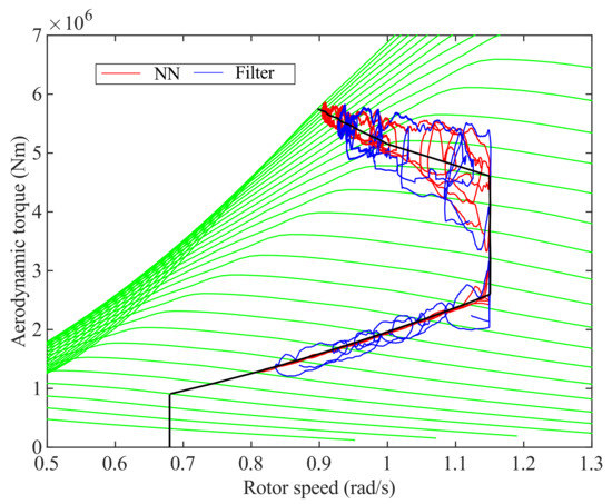
Figure 16.
Control operation results in torque-speed plane; refer to Figure 3 for the green wind speed curves.
Figure 17, Figure 18 and Figure 19 show the behaviour of Turbine 5 (selected randomly because the other turbines behave similarly) at mean wind speeds of 8 (mode 2; refer to Figure 3 for “modes”), 10 (mode 3), and 14 (mode 4) m/s, respectively, in the time-domain when the controller uses the aerodynamic torque estimated by the NN-based estimator (in red) compared to the case where the controller uses the aerodynamic torque estimated by the conventional aerodynamic torque estimator (in black). As shown in these figures, it is not straightforward to compare the two because the controllers are designed to track the full operational strategy curve in the torque-speed plane; that is, the torque-speed plane shown in Figure 16 should be used to facilitate a clearer comparison between the two as follows.
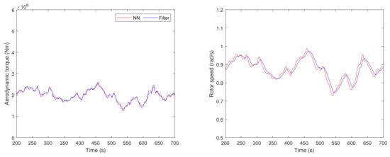
Figure 17.
Output at a mean wind speed of 8 m/s (mode 2).
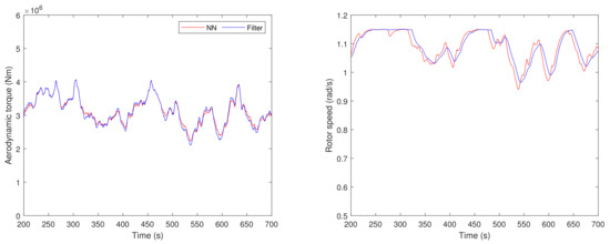
Figure 18.
Output at a mean wind speed of 10 m/s (mode 3).
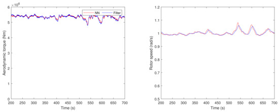
Figure 19.
Output at a mean wind speed of 14 m/s (mode 4).
Figure 16 shows the behaviour of Turbine 5 (selected randomly because the remaining turbines behave similarly) in the torque-speed plane over the full operational envelope, that is, from 8 to 16 m/s with an increment of 2 m/s when the NN-based estimator (in red) provides the controller with the estimation of aerodynamic torque compared to when the conventional aerodynamic torque estimator (in blue) provides the controller with the estimation. As can be seen, the full operational strategy curve is tracked more closely with the NN-based estimator. At each mean wind speed (i.e., over the full envelope), the wind turbine is simulated for 700 s to generate the results shown in the figure. Here, each green curve represents a mean wind speed, as clearly shown in Figure 3. In each mode, the controller tracks the full operational strategy curve more closely when the controller uses the aerodynamic torque estimated using the NN-based estimator, as is clearly demonstrated in the torque-speed plane.
Figure 20 shows the corresponding power efficiency of the controller for the below rated wind speed when the NN-based estimator (in red) is used, compared to when the conventional aerodynamic torque estimator (in blue) is used. These results demonstrate that efficiency is improved using the NN estimator. Here, the interpretation supports the results shown in Figure 16. Note that presenting the power efficiency in modes 3 and 4 is meaningless because the control role in these modes is to limit power rather than extracting as much power as possible.
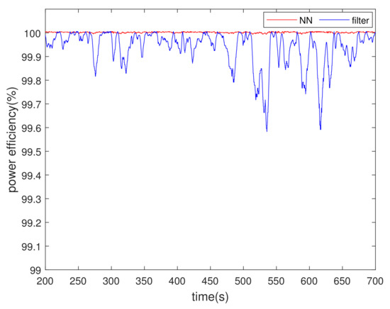
Figure 20.
Power efficiency in below rated wind speed.
The results for Scenarios 1 to 5 are summarised in Table 1. Estimations acquired by the NN-based estimator tracking actual measurements are quantified and compared with estimations acquired by the conventional wind speed and aerodynamic torque estimators tracking actual measurements, for each scenario. In line with the results demonstrated in Figure 6, Figure 7, Figure 8, Figure 9, Figure 10, Figure 11, Figure 12, Figure 13, Figure 14 and Figure 15, the table illustrates that estimations acquired by the NN-based estimator are closer to actual measurements than the estimates obtained by the conventional wind speed and aerodynamic torque estimators.

Table 1.
NN-based estimator vs filter-based estimator using error metrics.
Table 2 presents the control performance when the NN-based estimator provides the controller with the estimation of aerodynamic torque compared to when the conventional aerodynamic torque estimator provides the estimation using error metrics. As previously mentioned, in mode 2, the curve is tracked trying to extract as much energy as possible from the wind; in mode 3 the constant rotor speed () is tracked; and in mode 4 the rated power () is maintained by stalling the turbine. The table illustrates that: (i) in mode 2, the power efficiency is higher; (ii) in mode 3, the constant rotor speed is tracked more closely; and (iii) in mode 4, the rated power is tracked more closely when the NN-based estimator is in place, confirming the results demonstrated in Figure 16, Figure 17, Figure 18, Figure 19 and Figure 20.
Table 2.
Control performance in each mode.
5. Conclusions
In this paper, a simple method for estimating potentially useful (but typically unmeasured) variables in wind turbines and farms is proposed. Only a single turbine in a cluster of several wind turbines (five in this paper) is equipped with a sensor, and the remaining turbines are equipped with an NN based estimator, which would significantly reduce the associated costs. The turbine equipped with the sensor is used to train the NN-based estimator, which essentially replaces potentially expensive sensors. The proposed method can be used to estimate various variables; however, this paper focuses on wind speed and aerodynamic torque. The results of simulations demonstrate that estimations acquired by the NN-based estimator closely follow actual measurements and are closer to actual measurements than estimates obtained by the conventional wind speed and aerodynamic torque estimators.
Wind turbine controllers often utilise aerodynamic torque estimation, and this estimation is frequently performed using a conventional aerodynamic torque estimator, for example, the one described in Section 3.1. The new controller tested in this paper replaces the conventional aerodynamic torque estimator with the proposed NN-based estimator, and the resulting control output is compared to that of the original controller using the conventional aerodynamic torque estimator. The results demonstrate that the controller yields improved results when it uses the estimated aerodynamic torque obtained by the proposed NN-based estimator.
Further research in this field will include improving the control of wind turbines by incorporating the wind speed estimated by the proposed method and utilising the NN-based estimation method to estimate other variables that are hard or expensive to measure, to further improve control and condition monitoring of wind turbines. Furthermore, in this paper it is assumed that the wind turbines are aligned side by side, implying that the wake effects are not dominant. Future work will consider various different layouts, which could amplify the wake effects, and investigate how the proposed method is affected.
Author Contributions
Conceptualization, S.-h.H. and Y.-s.R.; methodology, S.-h.H.; software, Y.-s.R.; validation, S.-h.H. and Y.-s.R.; formal analysis, S.-h.H.; investigation, S.-h.H. and Y.-s.R.; resources, S.-h.H. and Y.-s.R.; data curation, Y.-s.R.; writing—original draft preparation, S.-h.H. and Y.-s.R.; writing—review and editing, S.-h.H.; visualization, S.-h.H. and Y.-s.R.; supervision, S.-h.H.; project administration, S.-h.H.; funding acquisition, S.-h.H. Both authors have read and agreed to the published version of the manuscript.
Funding
This work was supported in part by the Korea Institute of Energy Technology Evaluation and Planning (KETEP) grant funded by the Korean government (MOTIE) (20203010020010, Development and Demonstration of Integrated O&M Service Solution for Digital-Based Offshore Wind Power Plant) and the Korea Electric Power Corporation (R21XO01-17).
Institutional Review Board Statement
Not applicable.
Informed Consent Statement
Not applicable.
Data Availability Statement
Not applicable.
Conflicts of Interest
The authors declare no conflict of interest.
References
- Tiumentsev, Y.; Egorchev, M. Neural Network Modeling and Identification of Dynamical Systems; Academic Press: Cambridge, MA, USA, 2019. [Google Scholar]
- Aggarwa, C.C. Neural Networks and Deep Learning: A Textbook; Springer: Berlin/Heidelberg, Germany, 2018. [Google Scholar]
- Besancon, G. Nonlinear Observers and Applications; Springer: Berlin/Heidelberg, Germany, 2007. [Google Scholar]
- Goodwin, G.C. Adaptive Filtering Prediction and Control; Dover Publications: Mineola, NY, USA, 2009. [Google Scholar]
- Welling, M. The Kalman Filter; Technical Report; California Institute of Technology: Pasadena, CA, USA, 2010. [Google Scholar]
- Grewal, M.S.; Andrews, A.P. Kalman Filtering: Theory and Practice with MATLAB, 4th ed.; Wiley-IEEE Press: Hoboken, NJ, USA, 2015. [Google Scholar]
- Leithead, W.; Connor, B. Control of variable speed wind turbines: Dynamic models. Int. J. Control 2000, 73, 1173–1188. [Google Scholar] [CrossRef]
- Jiao, X.; Yang, Q.; Zhu, C.; Fu, L.; Chen, Q. Effective Wind Speed Estimation and Prediction Based Feedforward Feedback Pitch Control for Wind Turbines. In Proceedings of the 2019 12th Asian Control Conference (ASCC), Kitakyushu, Japan, 9–12 June 2019; pp. 799–804. [Google Scholar]
- Soltani, M.N.; Knudsen, T.; Svenstrup, M.; Wisniewski, R.; Brath, P.; Ortega, R.; Johnson, K. Estimation of Rotor Effective Wind Speed: A Comparison. IEEE Trans. Control Syst. Technol. 2013, 21, 1155–1167. [Google Scholar] [CrossRef]
- Deng, X.; Yang, J.; Sun, Y.; Song, D.; Yang, Y.; Joo, Y.H. An Effective Wind Speed Estimation Based Extended Optimal Torque Control for Maximum Wind Energy Capture. IEEE Access 2020, 8, 65959–65969. [Google Scholar] [CrossRef]
- Jena, D.; Rajendran, S. A review of estimation of effective wind speed based control of wind turbines. Renew. Sustain. Energy Rev. 2015, 43, 1046–1062. [Google Scholar] [CrossRef]
- Golnary, F.; Moradi, H. Dynamic modelling and design of various robust sliding mode controls for the wind turbine with estimation of wind speed. Appl. Math. Model. 2019, 65, 566–585. [Google Scholar] [CrossRef]
- Simley, E.; Fürst, H.; Haizmann, F.; Schlipf, D. Optimizing Lidars for Wind Turbine Control Applications—Results from the IEA Wind Task 32 Workshop. Remote Sens. 2018, 10, 863. [Google Scholar] [CrossRef]
- Barcena, R.; Acosta, T.; Etxebarria, A.; Kortabarria, I. LIDAR-Assisted Wind Turbine Structural Load Reduction by Linear Single Model Predictive Control. IEEE Access 2020, 8, 146548–146559. [Google Scholar] [CrossRef]
- Mirzaei, M.; Mann, J. Lidar configurations for wind turbine control. J. Phys. Conf. Ser. 2016, 753, 032019. Available online: https://iopscience.iop.org/article/10.1088/1742-6596/753/3/032019/pdf (accessed on 31 May 2021). [CrossRef]
- Hur, S.; Leithead, W. Collective control strategy for a cluster of stall-regulated offshore wind turbines. Renew. Energy 2016, 85, 1260–1270. [Google Scholar] [CrossRef]
- Maciejowski, J.M. Predictive Control with Constraints; Prentice Hall: Hoboken, NJ, USA, 2000. [Google Scholar]
- Rossiter, J.A. Model-Based Predictive Control: A Practical Approach; CRC Press: Boca Raton, FL, USA, 2005. [Google Scholar]
- Leithead, W.; Connor, B. Control of variable speed wind turbines: Design task. Int. J. Control 2000, 73, 1189–1212. [Google Scholar] [CrossRef]
- Leithead, W.E. Effective wind speed models for simple wind turbine simulations. In Proceedings of the 14th British Wind Energy Association (BWEA) Conference, Nottingham, UK, 25–27 March 1992. [Google Scholar]
- Acho, N.L.V. Wind Turbine Control and Monitoring; Springer: Cham, Switzerland, 2014. [Google Scholar]
- Ostergaard, K.Z.; Brath, P.; Stoustrup, J. Estimation of effective wind speed. J. Phys. Conf. Ser. 2007, 75, 012082. [Google Scholar] [CrossRef]
- Beale, M.H.; Hagan, M.T.; Demuth, H.B. Deep Learning Toolbox Getting Started Guide; Technical Report; MathWorks: Natick, MA, USA, 2020. [Google Scholar]
- Lawrynczuk, M. Computationally Efficient Model Predictive Control Algorithms: A Neural Network Approach; Springer: Berlin/Heidelberg, Germany, 2016. [Google Scholar]
- Lawrynczuk, M. Training of neural models for predictive control. Neurocomputing 2010, 73, 1332–1343. [Google Scholar] [CrossRef]
- Yu, H.; Wilamowski, B.M. The Industrial Electronics Handbook: Levenberg-Marquardt Training; Routledge Handbooks Online; CRC Press: Boca Raton, FL, USA, 2016. [Google Scholar]


Publisher’s Note: MDPI stays neutral with regard to jurisdictional claims in published maps and institutional affiliations. |
© 2021 by the authors. Licensee MDPI, Basel, Switzerland. This article is an open access article distributed under the terms and conditions of the Creative Commons Attribution (CC BY) license (https://creativecommons.org/licenses/by/4.0/).