Experimental Analysis and Prediction Model of Milling-Induced Residual Stress of Aeronautical Aluminum Alloys

Featured Application

This paper proposes a prediction model for milling residual stress based on a BP neural network. It aims to provide basic data calculation tools for analyzing the influence of milling residual stress on workpiece deformation, crack resistance, fatigue life, and corrosion resistance. Unlike traditional forecasting models, the prediction model is based on actual machining conditions. The prediction model contains the influence of various hidden factors, so it is closer to actual production. Additionally, the proposed model has a high prediction accuracy because of the strong nonlinear mapping ability of the BP neural network.

Abstract

Aeronautical thin-walled frame workpieces are usually obtained by milling aluminum alloy plates. The residual stress within the workpiece has a significant influence on the deformation due to the relatively low rigidity of the workpiece. To accurately predict the milling-induced residual stress, this paper describes an orthogonal experiment for milling 7075 aluminum alloy plates. The milling-induced residual stress at different surface depths of the workpiece, without initial stress, is obtained. The influence of the milling parameters on the residual stress is revealed. The parameters include milling speed, feed per tooth, milling width, and cutting depth. The experimental results show that the residual stress depth in the workpiece surface is within 0.12 mm, and the residual stress depth of the end milling is slightly greater than that of the side milling. The calculation models of residual stress and milling parameters for two milling methods are formulated based on regression analysis, and the sensitivity coefficients of parameters to residual stress are calculated. The residual stress prediction model for milling 7075 aluminum alloy plates is proposed based on a back-propagation neural network and genetic algorithm. The findings suggest that the proposed model has a high accuracy, and the prediction error is between 0–14 MPa. It provides basic data for machining deformation prediction of aluminum alloy thin-walled workpieces, which has significant application potential.

1. Introduction

Aeronautical aluminum alloy has a high specific strength, as well as excellent mechanical and machining properties. As an ideal structural material, it is widely used to manufacture aeronautical workpieces [1,2,3,4,5]. Thin-walled frame structures machined from aluminum alloy plates is the first choice for aeronautical workpieces to improve production efficiency and reduce product weight, assembly time, and production costs [6,7,8]. However, material removal of a thin-walled frame workpiece is large, and the workpiece stiffness after machining is low. During the machining process, the internal residual stress of the plate changes in a complicated way, which causes the workpiece to warp or twist after machining. The workpiece deformation causes a high rejection rate or additional correction procedures, which significantly increases production costs and reduces production efficiency [9,10,11]. The cutting-induced residual stress is an essential factor affecting workpiece deformation and accuracy stability [12]. As the residual stress increases, the thin-walled workpiece deformation increases [13]. In addition, the cutting-induced residual stress affects the service life and performance of the workpiece [14,15].

Residual stress is mainly caused by the combined effects of cutting force and cutting heat during the machining process [16]. Scholars have carried out a great deal of research on the machining-induced residual stress of structural parts. Shan et al. [17] proposed an improved prediction model for the residual stress of an orthogonal cutting process, considering the mechanical and thermal stress based on contact mechanics, the Johnson–Cook constitutive model, and the slip line theory. Starting from the geometric parameters of the milling cutter, Shen et al. [18] created a finite element model to investigate the influence of the cutting edge shape on the residual stress distribution in the machined surface. Ji et al. [19] studied the residual stress distribution in square pocket milling of 2219 aluminum alloy. They suggested that the axial cutting depth is the most critical factor influencing the residual stress distribution of the machined pocket surface. As the axial cutting depth increased, the tensile stress increased. The altered feed rate and radial cutting depth slightly affected the residual stress distribution and the average value. Liu et al. [20] pointed out that the plastic deformation caused by the cutting force is the dominant factor in the residual stress in ultra-precision machining 2024 aluminum alloy with a single crystal diamond tool. Salvati and Korsunsky [21] reconstructed the residual stress caused by the surface treatment based on the finite element method. Feature simplification reduces the amount of calculation during preprocessing by the finite element software. Meng et al. [22] investigated the effects of prestress on surface residual stress through milling experiments. Zhang et al. [23] studied the impact of milling width on surface residual stress using Al5Si aluminum alloy. Further, they explored the influence of milling thickness on the tensile anisotropy of hybrid wire arc additive-milling subtractive manufacturing. Xiong et al. [24] analyzed the residual stress of in situ milling of TiB2/7050Al metal matrix composites. They found that cutting temperature played a significant role in residual stress through comparative research. Huang et al. [25] proposed an analytical method for residual stress prediction in dynamic orthogonal cutting and formulated a dynamic orthogonal cutting mechanistic model considering the effect of cutting edge indentation. Based on plastic strain calculation and the inclusion theory, they formulated an analytical residual stress solution of the plastic strain distributed in the half-plane. Then, they predicted two-dimensional residual stress distribution in non-relaxation dynamic cutting and performed a dynamic cutting orthogonal experiment to verify the prediction results. Cheng et al. [26] studied surface residual stress under different cutting parameters and machining characteristics. They proposed a new method based on Gaussian process regression for predicting machining-induced surface residual stress, which was verified through comparison to other machine learning algorithms. Andrey et al. [27] studied the effect of repeated stress on hard milling using 3D finite element simulations. They investigated the formation of stresses at variable tooth feeds with a constant cutting speed and depth, and determined the development of material modifications (residual stresses) due to multiple stresses. Zhou et al. [28] presented an analytical model of residual stress generation in complex surface milling. Milling-introduced mechanical stress was determined according to the contact mechanics and the geometric transformation in the workpiece. The residual stress was estimated using an elastic–plastic model and a relaxation procedure. Additionally, the proposed model was verified through a milling experiment.

Cutting-induced residual stress causes workpiece deformation, significantly affecting performance. For example, the negative effect of tensile residual stress was revealed in terms of crack resistance, fatigue life, and corrosion resistance. Reducing residual stress can enhance material performance [29]. Therefore, it is necessary to measure and optimize residual stress distribution to evaluate the residual stress state in the machined surface, control the workpiece deformation, and improve its performance. For the characteristics of cutting-induced residual stress, the most widely used measurement technology is X-ray diffraction. The accuracy of this method reaches ±10 MPa, and it has become the international standard method for surface residual stress measurement. However, limited by the X-ray penetration ability, it is difficult to measure the residual stress distribution directly [30]. Moreover, using the measurement method to adjust the machining parameters for the required residual stress results in high time and economic costs. Previous studies on cutting-induced residual stress mainly used analytical methods, finite element methods, and experimental methods. They explored the influence law and prediction model of cutting force, cutting heat, tool geometric sizes, and some cutting parameters on residual stress under dry cutting conditions and orthogonal cutting process. However, the research on the influence law and prediction model of various factors on residual stress under wet cutting conditions and non-orthogonal cutting process is rarely involved. Milling aluminum alloy is generally under cooling conditions, which is non-orthogonal cutting. The simulation method is computationally intensive and time-consuming. The experimental method is time-consuming, laborious, and costly. In addition, it is necessary to repeatedly establish simulation models and implement experimental verification for parts with different characteristics and machining parameters.

Given the above issues, it is of engineering significance to study residual stress distribution and the prediction model under actual milling conditions. This paper takes 7075 aluminum alloy as the research object and performs experimental research on milling-induced residual stress. Firstly, the influence of milling parameters (e.g., milling speed, feed per tooth, milling width, and cutting depth) on the residual stress in end milling and side milling under a wet cutting condition is comparatively studied. Secondly, a back-propagation (BP) neural network with a strong nonlinear mapping ability is used to formulate the residual stress prediction model of milling aeronautical aluminum alloy based on the experimental data. Finally, the accuracy of the proposed prediction model is verified by experiments.

2. Milling-Induced Residual Stress Experiment of 7075 Aluminum Alloy

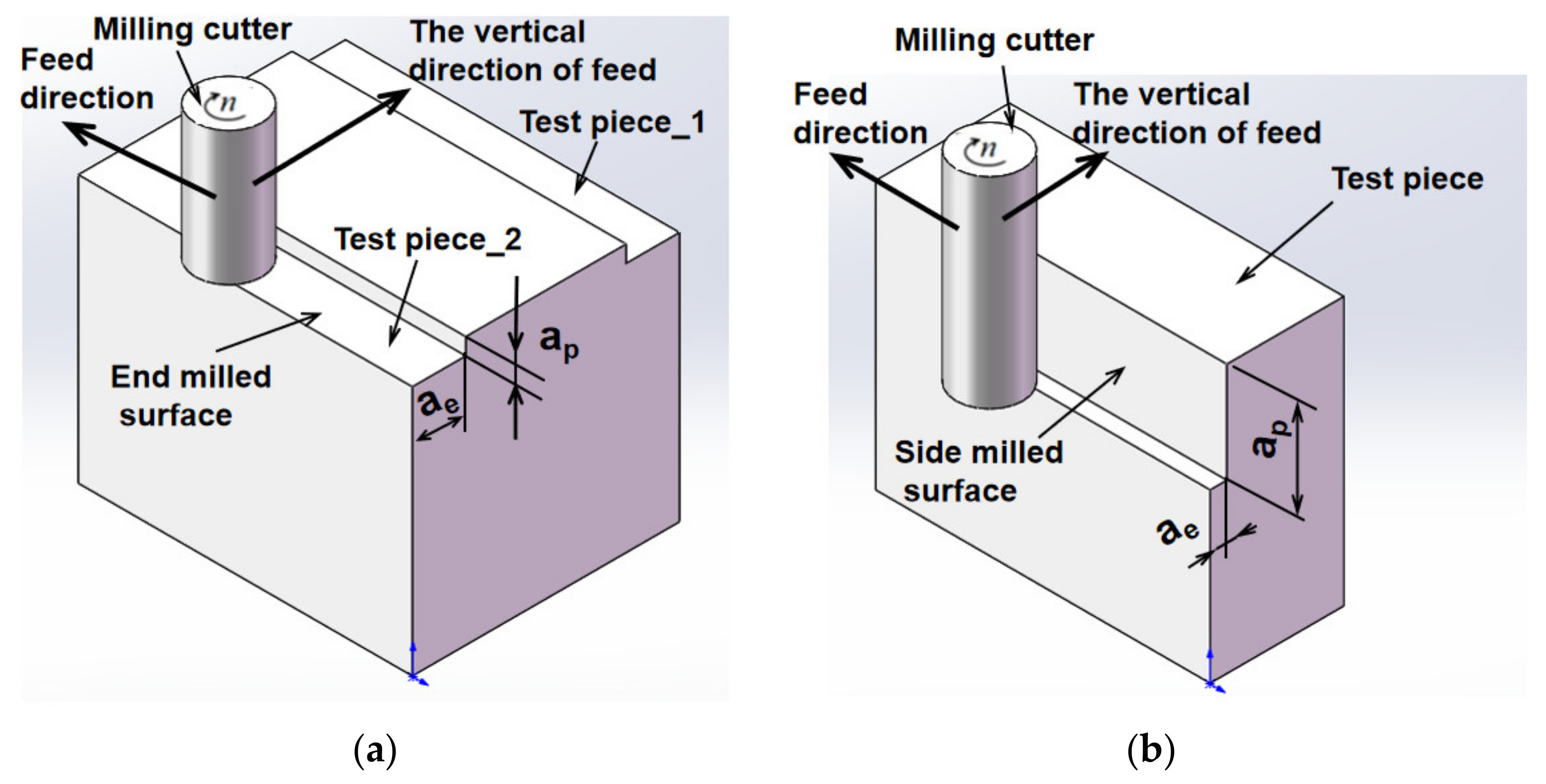
2.1. Design of the Experimental Study

The experimental material was a 7075-T7451 aluminum alloy pre-stretched plate. To save the time of preparing the test pieces, a type of test piece with 100 mm × 80 mm × 40 mm was cut out from the plate for an end milling experiment. A total of five test pieces were milled by the bottom edge of an end mill. Each test piece was subjected to two milling experiments with two sets of milling parameters. Each milling experiment was also performed at a different position of the test piece. Another type of test piece with a size of 100 mm × 40 mm × 40 mm was prepared for the side milling experiment, i.e., milling with the circumferential edge of an end mill. There were nine test pieces in total, and each test piece was only subjected to a milling experiment with one set of milling parameters. The two milling methods are shown in Figure 1.

Although the residual stress of Al7075-T7451 plate is about ±30 MPa, when it is superimposed with the milling stress, the milling stress cannot be distinguished. Therefore, before milling, the test pieces were subjected to stress relief annealing treatment to eliminate the influence of initial residual stress on the milling-induced residual stress. The temperature of annealing was about 350 °C. The initial stress of the annealed test pieces was tested and found to be around ±10 MPa, which can be regarded as a stress-free state.

The milling was carried out on a five-axis machining center of DMG-DMU-60-monoBLOCK, and the primary parameters are listed in

Table 1. The primary parameters of the five-axis machining center.

Parameters	Values
Stroke (mm)	X = 630, Y = 560, Z = 560
B-axis swing angle (°)	−120~+30
Maximum spindle speed (r/min)	12,000
Maximum feed rate of linear axis (mm/min)	30,000
Positioning accuracy (mm)	0.006
Control system	Heidenhain iTNC530

. The milling adopted the Heye-M2Al 4-blade-alloy milling cutter with a diameter of 20 mm, helix angle of 30°, rake angle of 15°, relief angle of 10°, and cutting edge of 50 mm.

Cutting oil was used to cool the tool during milling. The factors affecting the test piece deformation included milling speed, v_c; feed per tooth, f_z; milling width, a_e; and cutting depth, a_p. Thus, a four-factor three-level orthogonal milling experiment was adopted. Taking into account the performance of the selected tool and the range of commonly used finishing milling parameters, we selected three milling speeds (i.e., 125.6 m/min, 376.8 m/min, 628 m/min) and three levels of feed per tooth (i.e., 0.01 mm/z, 0.025 mm/z, 0.05 mm/z). For end milling, three milling depths (i.e., 0.5 mm, 1 mm, 1.5 mm) and three milling widths (i.e., 10 mm, 15 mm, 20 mm) were selected. For side milling, three milling depths (i.e., 15 mm, 25 mm, 35 mm) and three milling widths (i.e., 0.2 mm, 0.6 mm, 1 mm) were selected. The parameters of the end milling and side milling are presented in

Table 2. The parameters of the end milling experiment.

Test Piece Number	vc (m/min)	fz (mm)	ap (mm)	ae (mm)
1	125.6	0.01	0.5	10
2	125.6	0.025	1	15
3	125.6	0.05	1.5	20
4	376.8	0.01	1	20
5	376.8	0.025	1.5	10
6	376.8	0.05	0.5	15
7	628	0.01	1.5	15
8	628	0.025	0.5	20
9	628	0.05	1	10

and

Table 3. The parameters of the side milling experiment.

Test Piece Number	vc (m/min)	fz (mm)	ap (mm)	ae (mm)
1	125.6	0.01	15	0.2
2	125.6	0.025	25	0.6
3	125.6	0.05	35	1
4	376.8	0.01	25	1
5	376.8	0.025	35	0.2
6	376.8	0.05	15	0.6
7	628	0.01	35	0.6
8	628	0.025	15	1
9	628	0.05	25	2

.

2.2. Test Results of Milling-Induced Residual Stress

The residual stress in the surface of the milled test pieces was measured by X-ray diffraction. The test instrument was a XSTRESS-3000 residual stress analyzer made in Finland, with an accuracy of ±10 MPa. The parameters of the X-ray diffractometer are shown in

Table 4. XRD measurement parameters.

X-ray Diffraction Parameters	Specification/Values
Tube type	Cr
Supplied current during the experiment	6.7 mA
Supplied voltage during the experiment	30 kV
Exposure time for the calibration	8 s
Exposure time for measurement	10 s
Collimator diameter	3 mm
Collimator distance	10.390 mm
2-theta angle	138.75°
Tilt angle	−45° to 45°
Number of tilts	5/5
Rotation angle	0° to 90°
Number of rotations	2
Stress resolution	±10 MPa
Poisson ratio	0.33
Young’s modulus	70.3 GPa

. The residual stress of milling varied slightly with the milling position. The small ratio of the tool diameter to the spot diameter may affect measurement accuracy. To this end, we selected three test points on each machined surface of the test piece. In addition, the distance between two adjacent points was 25 mm, as shown in Figure 2. The residual stress average value at the three points was regarded as the milling-induced residual stress on the machined surface. An electrolytic polisher was used to polish the piece surface to obtain the residual stress distribution along the depth direction in the milled surface. The thickness of each polishing was 0.02 mm and the residual stress was measured layer by layer. A Kristall 650 electrolytic polishing machine maded in Germany was used for electrolytic polishing and the parameters are shown in

Table 5. Electrolytic polishing parameters.

Electrolytic Polishing Parameters	Specification/Values
Electrolyte	NaCl
Voltage	40 V
Flowrate	10
Working current	2 A
Area	63.59 mm2

. The residual stress distribution state corresponding to each milling parameter was obtained. We took the depth of the milling stress layer as the abscissa, and the residual stress value based on the experiment as the ordinate. Then, the spline function was employed for curve fitting in MATLAB. As a result, the residual stress distribution along the depth direction was obtained, as shown in Figure 3 and Figure 4. The residual stress in the machined surface was the result of many factors. The experimental results showed that the end milling-induced residual stress was within 0.12 mm of the test piece surface, and the side milling-induced residual stress was within 0.08 mm. The residual stress varied significantly along the depth direction, and the overall distribution was in a “spoon shape”. After reaching the maximum value at a depth of 0.02 mm, the residual stress gradually decreased with depth.

To conveniently analyze the influence of various milling parameters on residual stress, the residual stress at different depths under each group of parameters was equivalently treated using Equation (1). The results are listed in

Table 6. The equivalent results of the end milling-induced residual stress.

Test Piece Number	vc (m/min)	fz (mm/z)	ap (mm)	ae (mm)	${\mathit{\sigma }}_{\mathit{e}\mathit{n}\mathit{d}1}$ (MPa)	${\mathit{\sigma }}_{\mathit{e}\mathit{n}\mathit{d}2}$ (MPa)
1	125.6	0.01	0.50	10.00	−84.77	−67.56
2	125.6	0.025	1.00	15.00	−76.56	−61.18
3	125.6	0.05	1.50	20.00	−60.34	−36.40
4	376.8	0.01	1.00	20.00	−80.45	−58.48
5	376.8	0.025	1.50	10.00	−52.16	−48.36
6	376.8	0.05	0.50	15.00	−53.78	−39.35
7	628	0.01	1.50	15.00	−77.18	−38.26
8	628	0.025	0.50	20.00	−51.93	−31.72
9	628	0.05	1.00	10.00	−41.43	−36.46

and

Table 7. The equivalent results of the side milling-induced residual stress.

Test Piece Number	vc (m/min)	fz (mm/z)	ap (mm)	ae (mm)	${\mathit{\sigma }}_{\mathit{s}\mathit{i}\mathit{d}\mathit{e}1}$ (MPa)	${\mathit{\sigma }}_{\mathit{s}\mathit{i}\mathit{d}\mathit{e}2}$ (MPa)
1	125.6	0.01	15.00	0.20	−31.32	−25.17
2	125.6	0.025	25.00	0.60	−18.65	−12.17
3	125.6	0.05	35.00	1.00	−10.69	−8.74
4	376.8	0.01	25.00	1.00	−17.34	−10.40
5	376.8	0.025	35.00	0.20	−21.57	−14.96
6	376.8	0.05	15.00	0.60	−27.22	−16.17
7	628	0.01	35.00	0.60	−34.04	−21.65
8	628	0.025	15.00	1.00	−19.96	−18.86
9	628	0.05	25.00	0.20	−11.18	−11.49

. The maximum residual stress in the tables is 84.77 MPa, which is much smaller than the yield stress of the material, but will cause larger bending deformation of the weakly rigid thin-walled parts. The tool software, Design-Expert, was used for the variance analysis on the orthogonal data in Table 6 and Table 7, and the results are shown in

Table 8. The results of analysis of variance in the orthogonal experiment of end milling.

Source	The Feed Direction					The Vertical Direction of Feed
	SS	df	MS	F-Value	p-Value	SS	df	MS	F-Value	p-Value
Regression analysis	1616.59	4	404.15	4.91	0.0762	1177.22	4	294.31	6.97	0.0433
Vc	435.71	1	435.71	5.29	0.0829	574.28	1	574.28	13.59	0.0211
fz	1146.41	1	1146.41	13.93	0.0203	451.56	1	451.56	10.69	0.0308
ap	0.1067	1	0.1067	0.0013	0.973	40.61	1	40.61	0.9612	0.3824
ae	34.37	1	34.37	0.4176	0.5534	110.77	1	110.77	2.62	0.1807
Residual	329.24	4	82.31			169.01	4	42.25
Cor Total	1945.83	8				1346.23	8

and

Table 9. The results of analysis of variance in the orthogonal experiment of end milling.

Source	The Feed Direction					The Vertical Direction of Feed
	SS	df	MS	F-Value	p-Value	SS	df	MS	F-Value	p-Value
Regression analysis	245.43	4	61.36	0.8409	0.5647	143.36	4	35.84	1.45	0.3638
Vc	3.41	1	3.41	0.0467	0.8395	5.84	1	5.84	0.2363	0.6523
fz	174.12	1	174.12	2.39	0.1973	69.84	1	69.84	2.83	0.1681
ap	24.81	1	24.81	0.34	0.5911	36.75	1	36.75	1.49	0.2897
ae	43.09	1	43.09	0.5906	0.4851	30.92	1	30.92	1.25	0.326
Residual	291.87	4	72.97			98.88	4	24.72
Cor Total	537.31	8				242.24	8

. Generally, a p-value less than 0.05 indicates that the model term is significant, while a p-value greater than 0.1 indicates that the model term is not significant. The results in Table 8 suggest that f_z is a significant model item for the feed direction of end milling, and f_z and v_c are significant model items for the vertical direction of feed of end milling.

Then, linear regression analysis was used to fit the empirical formula of the milling-induced residual stress of 7075 aluminum alloy. Through the orthogonal experiments, the exponential relationship between the residual stress and milling parameters was formulated as Equations (2)–(5).

$${\sigma }_{\mathrm{equ}}={{\displaystyle \int }}_0^h\sigma dh/H,$$

(1)

where H is the depth of the milling-induced residual stress.

$${\sigma }_{end1}=-38.0195v_c^{-0.176}{f}_z^{-0.2827}{a}_p^{0.0108}{a}_e^{0.1732},$$

(2)

$${\sigma }_{end2}=-156.6478v_c^{-0.2277}{f}_z^{-0.2081}{a}_p^{-0.0383}{a}_e^{-0.269},$$

(3)

where ${\sigma }_{end1}$, ${\sigma }_{end2}$ denote the equivalent residual stress in the feed direction and vertical direction of feed of end milling, respectively; $125.6 \mathrm{m}/\min \le v_c\le 628 \mathrm{m}/\min ,$ $0.01\mathrm{mm}/\mathrm{z}\le f_z\le 0.05$ mm/z, $0.5\mathrm{mm}\le a_p\le 1.5 \mathrm{mm}$, $10\mathrm{mm}\le a_e\le 25 \mathrm{mm}$.

$${\sigma }_{side1}=-11.8627v_c^{0.0577}{f}_z^{-0.3428}{a}_p^{-0.362}{a}_e^{-0.0843},$$

(4)

$${\sigma }_{side2}=-12.8353v_c^{0.0947}{f}_z^{-0.2419}{a}_p^{-0.449}{a}_e^{-0.162},$$

(5)

where ${\sigma }_{side1}$, ${\sigma }_{side2}$ denote the equivalent residual stress in the feed direction and vertical direction of feed of side milling, respectively; $125.6 \mathrm{m}/\min \le v_c\le 628 \mathrm{m}/\min$, $0.01\mathrm{mm}/\mathrm{z}\le f_z\le 0.05 \mathrm{mm}/\mathrm{z}$, $15\mathrm{mm}\le a_p\le 35 \mathrm{mm}$, $0.2\mathrm{mm}\le a_e\le 1\mathrm{mm}$.

The four formulas indicate that the equivalent residual stress in milling is expressed as compressive stress.

(1)

The condition of end milling.

According to Equations (2) and (3), the significance of the milling parameters to the residual stress in the feed direction is $f_z>v_c>a_e>a_p$, and the significance of the parameters to the residual stress in the vertical direction of feed is $a_e>v_c>f_z>a_p$. When $v_c$ and $f_z$ increase, the residual stress in the two directions exhibits a decreasing trend. When $a_p$ and $a_e$ increase, the residual stress in the feed direction increases, and the residual stress in the vertical direction of feed decreases.

(2)

The condition of side milling.

According to Equations (4) and (5), the significance of the parameters to the residual stress in the two directions is $a_p>f_z>a_e>v_c$. When $n$ increases, the residual stress in the two directions increases. When$f_z$, $a_p$ and $a_e$ increase, the residual stress in the two directions decreases.

Note that, except for Equation (2), the p-values of the other three equations are all greater than 0.05. It shows that the regression effect is not significant. Thus, it is necessary to develop better analysis methods.

3. Prediction Model of Milling-Induced Residual Stress

3.1. Formulation of BP Neural Network

The BP neural network model consists of an input layer, a hidden layer and an output layer. The function of $\mathrm{newff}\left(\right)$ is used to formulate the model, expressed as:

$$\mathrm{net}=\mathrm{newff}\left(\mathrm{PR},\left[\mathrm{S}1\mathrm{S}{2}_{\cdots }\mathrm{SN}\right],\left\{\mathrm{TF}1\mathrm{TF}{2}_{\cdots }\mathrm{TFN}\right\},\mathrm{BTF},\mathrm{BLF},\mathrm{PF}\right),$$

(6)

where PR denotes a matrix of $\mathrm{R}\times 2$ to define the value range of R number of input vectors; [S1 S2…SN] is the number of neurons in each layer of the neural network; {TF1 TF2…TFN} represents the transfer function of each layer; by default, “tansig” and “purelin” are the transfer functions of the hidden layer and output layer, respectively; BLF reflects the learning of weights/thresholds, using the “learngdm” function; PF is the performance function, using the “mse” function. The input sample is transferred to PR after normalization, and PR is written as $\mathrm{minmax}\left(\mathrm{inputn}\right)$.

This study involves five factors: cutting speed, feed per tooth, back-cutting, cutting width, and milling stress layer depth. Modeling mainly considers the relationship between the five factors and the milling-induced residual stress. Thus, the input layer is designed with five neurons, corresponding to the five factors. The output layer has one neuron corresponding to the residual stress. The three-layer BP neural network with a hidden layer is used to predict the workpiece residual stress. By changing the number of neurons in the hidden layer, the error of the training process under different numbers is comparatively analyzed. Based on the principle of minor error, the number of hidden layer neurons is determined as fifteen. Thus, the function is formulated as Equation (7).

$$\mathrm{net}=\mathrm{newff}\left(\mathrm{minmax}\left(\mathrm{inputn}\right),\left[151\right],\left\{‘\tan \mathrm{sig}’,‘\mathrm{purelin}’\right\},‘\mathrm{traingdx}’,‘\mathrm{learngdm}’‘\mathrm{mse}’\right),$$

(7)

The specific operation steps of the BP neural network are as follows:

Step 1: network initialization. Each connection weight is assigned a random number in the interval [–1, 1]; the error function $e$, calculation accuracy $\mathsf{\epsilon }$, and maximum learning times $M$ are given.

Step 2: the input and output of the hidden layer and output layer are calculated as

$$h{i}_p\left(k\right)={\displaystyle \sum }_{i=1}^5{\mathrm{w}}_{hi}{\mathrm{x}}_i\left(k\right)+{\mathrm{b}}_p,$$

(8)

where p is the number of hidden layers, $p$= 1, 2, …, 15; i is the number of input variables, $h$ = 1, 2, 3, …, $p$; k is the number of samples, $k$= 1, 2, …, 63 represents 63 samples of end milling; $h{i}_p\left(k\right)$ is the input of the hidden layer; ${\mathrm{w}}_{hi}$ is the connection weight between the input layer and the hidden layer; ${\mathrm{b}}_p$ denotes the threshold of the hidden layer.

$$h{o}_p\left(k\right)=\mathrm{tansig}\left(h{i}_p\left(k\right)\right),$$

(9)

where $h{o}_p\left(k\right)$ is the output of the hidden layer.

$$yi\left(k\right)={\displaystyle \sum }_{p=1}^{15}{w}_{ho}h{o}_p\left(k\right)+{\mathrm{b}}_{\mathrm{o}},$$

(10)

where $yi\left(k\right)$ is the input of the output layer, $w_{oh}$ is the connection weight between the hidden layer and the output layer, and ${\mathrm{b}}_{\mathrm{o}}$ is the threshold of the output layer.

$$y\mathrm{o}\left(k\right)=\mathrm{purelin}\left(yi\left(k\right)\right),$$

(11)

where $yo\left(k\right)$ is the output of the output layer.

Step 3: the partial derivative ${\delta }_o\left(k\right)$ of the error function to each neuron in the output layer is calculated as:

$$\frac{\partial e}{\partial w_{oh}}=\frac{\partial e}{\partial yi}\frac{\partial yi}{\partial w_{oh}},$$

(12)

$$\frac{\partial yi}{\partial w_{oh}}=\frac{\partial \left({{\displaystyle \sum }}_h^{15}{w}_{oh}h{o}_h\left(k\right)-b_0\right)}{\partial w_{oh}}=h{o}_h\left(k\right),$$

(13)

$$\frac{\partial e}{\partial yi}=\frac{\partial {\left(\frac{1}{2}\left(d_o\left(k\right)-yo\left(k\right)\right)\right)}^2}{\partial yi}=-\left(d_o\left(k\right)-yo\left(k\right)\right)\mathrm{purelin}\prime (yi\left(k\right)-{\delta }_0\left(k\right),$$

(14)

where $d_o\left(k\right)$ represents the expected output.

$$\frac{\partial e}{\partial h{i}_h\left(k\right)}=-{\delta }_o\left(k\right)w_{ho}\mathrm{tansig}\prime \left(h{i}_p\left(k\right)\right)\triangleq -{\delta }_h\left(k\right),$$

(15)

Step 4: the connection weight $\Delta w_{oh}\left(k\right)$ is modified using ${\delta }_o\left(k\right)$ of each neuron in the output layer and the output of each neuron in the hidden layer.

$$\Delta w_{oh}\left(k\right)=-\mu \frac{\partial e}{\partial w_{oh}}=\mu {\delta }_o\left(k\right)h{o}_h\left(k\right),$$

(16)

where $\mu$ is the given learning rate.

$$w_{oh}^{N+1}=w_{oh}^N+\mu {\delta }_o\left(k\right)h{o}_h\left(k\right),$$

(17)

Step 5: the connection weight $\Delta w_{ih}\left(k\right)$ is modified using ${\delta }_h\left(k\right)$ of each neuron in the hidden layer and the input of each neuron in the input layer.

$$\Delta w_{hi}\left(k\right)=-\mu \frac{\partial e}{\partial w_{hi}}=-\mu \frac{\partial e}{\partial h{i}_h\left(k\right)}\frac{\partial h{i}_h\left(k\right)}{\partial w_{hi}}={\delta }_h\left(k\right)x_i\left(k\right),$$

(18)

$$w_{hi}^{N+1}=w_{hi}^N+\mu {\delta }_h\left(k\right)x_i\left(k\right),$$

(19)

Step 6: the global error is calculated as:

$$E=\frac{1}{126}{\displaystyle \sum }_{k=1}^{63}{(d_o\left(k\right)-y_o\left(k\right))}^2,$$

(20)

Step 7: Convergence judgment. If the error requirements are met and the maximum number of training times is reached, the learning ends; otherwise, the next learning cycle starts.

To investigate the performance of the formulated neural network, we implemented predictions based on the training data and observe the errors of the prediction model. The prediction results are shown in Figure 5. The results show that the prediction results obtained from the BP neural network are not ideal. The error on several samples is significant, and the absolute error exceeds 20 MPa. It is because the BP neural network may converge to a local minimum.

3.2. BP Neural Network Optimized by Genetic Algorithm

To deal with the problem of BP neural network converging to a local minimum, this study uses the genetic algorithm to optimize the neural network, thereby improving the convergence speed and reducing the prediction error. After optimization using the genetic algorithm, the weights and thresholds of the data in the end milling and side milling are obtained. The BP neural network prediction model is determined accordingly. We used the optimized model to implement predictions based on the training data. The prediction results are shown in Figure 6. The absolute error of the optimized prediction model is within ±6 MPa, which is consistent with the expected output. This verifies the effectiveness of the genetic algorithm for optimizing neural networks.

3.3. Validation of BP Neural Network Model

To verify the accuracy of the residual stress prediction model, six groups of data were re-selected for the milling experiment, three groups for end milling and three groups for side milling. The experimental parameters are listed in

Table 10. The experimental parameters for the validation of residual stress prediction model in the end milling.

Test Piece Number	vc (m/min)	fz (mm/z)	ap (mm)	ae (mm)
1	188.4	0.04	0.5	15
2	251.2	0.02	1.2	12
3	376.8	0.04	0.6	13

and

Table 11. The experimental parameters for the validation of residual stress prediction model in the side milling.

Test Piece Number	vc (m/min)	fz (mm/z)	ap (mm)	ae (mm)
1	188.4	0.01	15	0.2
2	251.2	0.02	18	0.5
3	376.8	0.03	24	0.9

, and the results are shown in Figure 7, Figure 8 and Figure 9. Figure 7 and Figure 8 show that the residual stress distribution curve obtained by the prediction model is consistent with the curve measured by the experiment. Figure 9 presents that the residual stress prediction absolute error of end milling is between 0.24–13.30 MPa, and that of side milling is between 0.23–11.34 MPa. The prediction error is in the same order of magnitude (i.e., ±10 MPa) as the measurement accuracy of the residual stress analyzer used. Therefore, the proposed prediction model of milling-induced residual stress is accurate.

4. Conclusions

This paper studies the influence of milling parameters on the residual stress of 7075 aluminum alloy and formulates a residual stress prediction model related to the parameters. It provides a calculation tool for obtaining milling-induced residual stress. First, the orthogonal experiment is designed to implement milling experiments on 7075 aluminum alloy. Through electrolytic polishing and X-ray diffraction, layer by layer, the workpiece residual stress distribution at different depths was obtained. Secondly, the residual stress characterization equations related to the milling parameters in end milling and side milling are formulated based on regression analysis. The sensitivity coefficient of each milling parameter to the residual stress is calculated. Thirdly, the prediction model of milling-induced residual stress is proposed based on experimental data, using a genetic algorithm and BP neural network. The findings indicate that milling-induced residual stress varies significantly along the workpiece depth direction. The residual stress depth is within 0.12 mm of the workpiece surface, and the overall distribution is in a “spoon shape”. The proposed prediction model can calculate the residual stress under different milling parameters. The prediction error is between 0–14 MPa, roughly the same as the measurement accuracy of the residual stress analyzer. Therefore, the prediction model has high accuracy and powerful application potential. In addition, this study gives constant values to factors, such as cutting tools, workpiece materials, and cooling conditions, resulting in limitations in the prediction model. In the future, we will incorporate more factors affecting milling-induced residual stress into the prediction model to improve its generality. In addition, the reverse approach of the optimal machining plan under the specified residual stress will be our research focus.

5. Replication of Results

In order to facilitate the reproduction of results presented in this paper, the MATLAB code is provided as the Supplementary Materials. The basic information of the code files is listed in

Table 12. The code files in the Supplementary Materials.

Filename	Description
ED-RS.xlsx	Experimental data on residual stress
VD-RS.xlsx	Verification data of residual stress experiment
P_ESRS.m	Calculation program of equivalent side milling residual stress
P_EERS.m	Calculation program of equivalent end milling residual stress
Basic data for(eq.2-eq.5).xlsx	Basic data for Equations (2)–(5)
CC_EQ2_3.m	Procedure for calculating the coefficients and exponents of Equations (2) and (3)
CC_EQ4_5.m	Procedure for calculating the coefficients and exponents of Equations (4) and (5)
Main_BP_TP_E_FD.m	Training program of BP neural network for residual stress in feed direction in end milling mode
Main_BP_TP_E_VFD.m	Training program of BP neural network for residual stress in vertical feed direction in end milling mode
Main_BP_TP_S_FD.m	Training program of BP neural network for residual stress in feed direction in side milling mode
Main_BP_TP_S_VFD.m	Training program of BP neural network for residual stress in vertical feed direction in side milling mode
Main_BP_PP_E_FD.m	BP neural network prediction program for residual stress in feed direction in end milling mode
Main_BP_PP_E_VFD.m	BP neural network prediction program for residual stress in vertical feeding direction in end milling mode
Main_BP_PP_S_FD.m	BP neural network prediction program for residual stress in feed direction in side milling mode
Main_BP_PP_S_VFD.m	BP neural network prediction program for residual stress in vertical feeding direction in side milling mode
BP-END-feed direction.rar	Summary of BP neural network program for residual stress in the feed direction of end milling
BP-END-vertical feed direction.rar	Summary of BP neural network program for residual stress in the vertical feed direction of end milling
BP-SIDE-feed direction.rar	Summary of BP neural network program for residual stress in the feed direction of side milling
BP-SIDE-vertical feed direction.rar	Summary of BP neural network program for residual stress in the vertical feed direction of side milling

. The detailed description is written as the comments in corresponding files. Notes that, the program package of ‘bcs_BP.rar’ needs to be extracted into a folder, which should be added into the search path of MATLAB.

References

1. Duan, Z.; Li, C.; Ding, W.; Zhang, Y.; Yang, M.; Gao, T.; Cao, H.; Xu, X.; Wang, D.; Mao, C.; et al. Milling Force Model for Aviation Aluminum Alloy: Academic Insight and Perspective Analysis. Chin. J. Mech. Eng. 2021, 34, 18. [Google Scholar] [CrossRef]
2. Li, H.; Jia, L.; Huang, J.; Ma, Y. Precipitation behavior and properties of extruded 7136 aluminum alloy under different aging treatments. Chin. J. Aeronaut. 2021, 34, 612–619. [Google Scholar] [CrossRef]
3. Chatterjee, B.; Bhowmik, S. Evolution of material selection in commercial aviation industry—A review. Sustain. Eng. Prod. Manuf. Technol. 2019, 199–219. [Google Scholar] [CrossRef]
4. Ji, M.; Li, W.; Liu, H.; Zhu, L.; Chen, H.; Li, W. Effect of titanium sol on sulfuric-citric acids anodizing of 7150 aluminum alloy. Surf. Interfaces 2020, 19, 100479. [Google Scholar] [CrossRef]
5. He, S.; Chen, S.; Zhao, Y.; Qi, N.; Zhan, X. Study on the intelligent model database modeling the laser welding for aerospace aluminum alloy. J. Manuf. Process. 2021, 63, 121–129. [Google Scholar] [CrossRef]
6. Zhang, J.; Cheng, X.; Xia, Q.; Yan, C. Strengthening effect of laser shock peening on 7075-T6 aviation aluminum alloy. Adv. Mech. Eng. 2020, 12, 1687814020952177. [Google Scholar] [CrossRef]
7. Zhong, H.; Liu, Z.; Qin, H.; Liu, Y. Static analysis of thin-walled space frame structures with arbitrary closed cross-sections using transfer matrix method. Thin Walled Struct. 2018, 123, 255–269. [Google Scholar] [CrossRef]
8. Sedeh, M.R.N.; Ghaei, A. The effects of machining residual stresses on springback in deformation machining bending mode. Int. J. Adv. Manuf. Technol. 2021, 114, 1087–1098. [Google Scholar] [CrossRef]
9. Sahraei, A.; Pezeshky, P.; Sasibut, S.; Rong, F.; Mohareb, M. Closed form solutions for shear deformable thin-walled beams including global and through-thickness warping effects. Thin Walled Struct. 2021, 158, 107190. [Google Scholar] [CrossRef]
10. Singh, A.; Agrawal, A. Comparison of deforming forces, residual stresses and geometrical accuracy of deformation machining with conventional bending and forming. J. Mater. Process. Technol. 2016, 234, 259–271. [Google Scholar] [CrossRef]
11. Santos, M.C.; Machado, A.R.; Sales, W.F.; Barrozo, M.A.S.; Ezugwu, E.O. Machining of aluminum alloys: A review. Int. J. Adv. Manuf. Technol. 2016, 86, 3067–3080. [Google Scholar] [CrossRef]
12. Ruitao, P.; Linfeng, Z.; Jiawei, T.; Xiuli, F.; Meiliang, C. Application of pre-stressed cutting to aviation alloy: The effect on residual stress and surface roughness. J. Manuf. Process. 2021, 62, 501–512. [Google Scholar] [CrossRef]
13. Zhang, Z.; Luo, M.; Tang, K.; Zhang, D. A new in-processes active control method for reducing the residual stresses induced deformation of thin-walled parts. J. Manuf. Process. 2020, 59, 316–325. [Google Scholar] [CrossRef]
14. Li, J.G.; Wang, S.Q. Distortion caused by residual stresses in machining aeronautical aluminum alloy parts: Recent advances. Int. J. Adv. Manuf. Technol. 2017, 89, 997–1012. [Google Scholar] [CrossRef]
15. Guo, J.; Fu, H.; Pan, B.; Kang, R. Recent progress of residual stress measurement methods: A review. Chin. J. Aeronaut. 2021, 34, 54–78. [Google Scholar] [CrossRef]
16. Mirkoohi, E.; Bocchini, P.; Liang, S.Y. Inverse analysis of residual stress in orthogonal cutting. J. Manuf. Process. 2019, 38, 462–471. [Google Scholar] [CrossRef]
17. Shan, C.; Zhang, M.; Zhang, S.; Dang, J. Prediction of machining-induced residual stress in orthogonal cutting of Ti6Al4V. Int. J. Adv. Manuf. Technol. 2020, 107, 2375–2385. [Google Scholar] [CrossRef]
18. Shen, Q.; Liu, Z.; Hua, Y.; Zhao, J.; Lv, W.; Hassan Mohsan, A.U. Effects of cutting edge micro-geometry on residual stress in orthogonal cutting of Inconel 718 by FEM. Materials 2018, 11, 1015. [Google Scholar] [CrossRef] [Green Version]
19. Ji, C.; Sun, S.; Lin, B.; Fei, J. Effect of cutting parameters on the residual stress distribution generated by pocket milling of 2219 aluminum alloy. Adv. Mech. Eng. 2018, 10, 1687814018813055. [Google Scholar] [CrossRef]
20. Liu, X.; Xiong, R.; Xiong, Z.; Zhang, S.; Zhao, L. Simulation and experimental study on surface residual stress of ultra-precision turned 2024 aluminum alloy. J. Braz. Soc. Mech. Sci. Eng. 2020, 42, 1–7. [Google Scholar] [CrossRef]
21. Salvati, E.; Korsunsky, A.M. A simplified FEM eigenstrain residual stress reconstruction for surface treatments in rbitrary 3D geometries. Int. J. Mech. Sci. 2018, 4, 138–139. [Google Scholar]
22. Meng, L.; Khan, A.M.; Zhang, H.; Fang, C.; He, N. Research on surface residual stresses generated by milling Ti6Al4V alloy under different pre-stresses. Int. J. Adv. Manuf. Technol. 2020, 107, 2597–2608. [Google Scholar] [CrossRef]
23. Zhang, S.; Gong, M.; Zeng, X.; Gao, M. Residual stress and tensile anisotropy of hybrid wire arc additive-milling subtractive manufacturing. J. Mater. Process. Technol. 2021, 293, 117077. [Google Scholar] [CrossRef]
24. Xiong, Y.; Wang, W.; Shi, Y.; Jiang, R.; Shan, C.; Liu, X.; Link, K. Investigation on surface roughness, residual stress and fatigue property of milling in-situ TiB2/7050Al metal matrix composites. Chin. J. Aviat. 2021, 34, 451–464. [Google Scholar] [CrossRef]
25. Huang, X.; Zhang, X.; Leopold, J.; Ding, H. Analytical Model for Prediction of Residual Stress in Dynamic Orthogonal Cutting Process. ASME J. Manuf. Sci. Eng. 2018, 140, 011002. [Google Scholar] [CrossRef]
26. Cheng, M.; Jiao, L.; Yan, P.; Feng, L.; Qiu, T.; Wang, X.; Zhang, N. Prediction of surface residual stress in end milling with Gaussian process regression. Measurement 2021, 178, 109333. [Google Scholar] [CrossRef]
27. Vovk, A.; Sölter, J.; Karpuschewski, B. Finite element simulations of the material loads and residual stresses in milling utilizing the CEL method. Procedia CIRP 2020, 87, 539–544. [Google Scholar] [CrossRef]
28. Zhou, R.; Yang, W. Analytical modeling of machining-induced residual stresses in milling of complex surface. Int. J. Adv. Manuf. Technol. 2019, 105, 565–577. [Google Scholar] [CrossRef]
29. Reimer, A.; Luo, X. Prediction of residual stress in precision milling of AISI H13 steel. Procedia CIRP 2018, 71, 329–334. [Google Scholar] [CrossRef]
30. Morin, L.; Braham, C.; Tajdary, P.; Seddik, R.; Gonzalez, G. Reconstruction of heterogeneous surface residual-stresses in metallic materials from X-ray diffraction measurements. Mech. Mater. 2021, 158, 103882. [Google Scholar] [CrossRef]
Figure 1. The end milling and side milling: (a) the end milling; (b) the side milling.
Applsci 11 05881 g001
Figure 2. The three test points on the milled surface.
Applsci 11 05881 g002
Figure 3. The residual stress distribution along the depth direction in the test piece surface of end milling: (a) the residual stress distribution in the feed direction; (b) the residual stress distribution in the vertical direction of feed.
Applsci 11 05881 g008
Figure 4. The residual stress distribution along the depth direction in the test piece surface of side milling: (a) the residual stress distribution in the feed direction; (b) the residual stress distribution in the vertical direction of feed.
Applsci 11 05881 g009
Figure 5. The prediction results of the BP neural network: (a) the prediction results; (b) the prediction error.
Applsci 11 05881 g003
Figure 6. The prediction results of the BP neural network optimized by genetic algorithm: (a) the prediction results; (b) the prediction error.
Applsci 11 05881 g004
Figure 7. The end milling experimental results: (a) the validation of prediction model in the feed direction; (b) the validation of prediction model in the vertical direction of feed.
Applsci 11 05881 g005
Figure 8. The side milling experimental results: (a) the validation of prediction model in the feed direction; (b) the validation of prediction model in the vertical direction of feed.
Applsci 11 05881 g006
Figure 9. The prediction error: (a) the prediction error of the end milling prediction model; (b) the prediction error of the side milling prediction model.
Applsci 11 05881 g007