Semiconductor Laser Linewidth Theory Revisited

Abstract

More and more applications require semiconductor lasers distinguished not only by large modulation bandwidths or high output powers, but also by small spectral linewidths. The theoretical understanding of the root causes limiting the linewidth is therefore of great practical relevance. In this paper, we derive a general expression for the calculation of the spectral linewidth step by step in a self-contained manner. We build on the linewidth theory developed in the 1980s and 1990s but look from a modern perspective, in the sense that we choose as our starting points the time-dependent coupled-wave equations for the forward and backward propagating fields and an expansion of the fields in terms of the stationary longitudinal modes of the open cavity. As a result, we obtain rather general expressions for the longitudinal excess factor of spontaneous emission (K-factor) and the effective $\alpha$-factor including the effects of nonlinear gain (gain compression) and refractive index (Kerr effect), gain dispersion, and longitudinal spatial hole burning in multi-section cavity structures. The effect of linewidth narrowing due to feedback from an external cavity often described by the so-called chirp reduction factor is also automatically included. We propose a new analytical formula for the dependence of the spontaneous emission on the carrier density avoiding the use of the population inversion factor. The presented theoretical framework is applied to a numerical study of a two-section distributed Bragg reflector laser.

1. Introduction

Many applications of semiconductor lasers utilized in miniaturized contemporary photonic integrated devices for coherent optical communication, optical atomic clocks, atom interferometry, gravitational wave detection, space-based metrology, and optical quantum sensing impose strict requirements on the coherence of the light source, which can be expressed in terms of the spectral linewidth. The theoretical understanding of the governing factors limiting the linewidth is therefore of great practical relevance. After a first prediction by Schawlow and Townes [1], the corresponding theoretical framework was developed in the 1960s [2,3,4,5,6]). Later, in the 1980s and 1990s with the rapidly advancing technology of the fabrication of semiconductor lasers and their applications the theory of the spectral linewidth was further refined. The following five milestones can be distinguished:

(i)

The first milestone is the discovery of the enhancement of the fraction of the spontaneous emission going into the lasing mode in gain-guided lasers and the derivation of a corresponding excess factor (K-factor) by Petermann [7]. Siegman recognized this effect as a general property of non-Hermitian laser cavities [8]. Later his discussion of the power-nonorthogonality of the transversal modes and its consequences was extended to the case of the power-nonorthogonality of the longitudinal modes of laser cavities [9]. In Ref. [10] it was discovered, that the longitudinal modes can become degenerate for certain parameter configurations resulting in an infinite K-factor. The occurrence of such exceptional points is not restricted to lasers but is inherent to non-Hermitian systems, see [11] for a recent review.

(ii)

The second milestone is the discovery of a linewidth enhancement in semiconductor gain materials caused by refractive index fluctuations in response to fluctuations of the carrier density. Due to gain clamping, intensity fluctuations (which have negligible direct effect on the linewidth) can cause substantial refractive index changes, which in turn lead to fluctuations of the phase. The magnitude of this amplitude-phase coupling is quantified by the linewidth enhancement factor ${\alpha }_{\mathrm{H}}$ or $\alpha$-factor introduced by Henry [12]. Later it was found that in DFB lasers the $\alpha$-factor has to be replaced by an effective factor ${\alpha }_{\mathrm{H},\mathrm{eff}}$ [13] and a general expression for ${\alpha }_{\mathrm{H},\mathrm{eff}}$ valid for distributed feedback (DFB), distributed Bragg reflector (DBR) and external cavity lasers was derived in [14].

(iii)

The third milestone is the discovery of the possibility of linewidth reduction due to optical feedback from an external cavity by Patzak et al. [15]. Later a relation to the reduction of the frequency chirp was established [16,17].

(iv)

The forth milestone is related to the deterioration of the linewidth due to charge carriers injected into a phase tuning section within the cavity. Amann and Schimpe figured out that carrier noise is the origin resulting in an additional contribution to the linewidth, if the $\alpha$-factors are different in the gain and phase tuning sections [18].

(v)

The last milestone is the discovery of the enhancement of the linewidth due to fluctuations of the shape of the profile of the optical power in the cavity by Tromborg and co-workers [14], which is particularly important in the vicinity of instabilities [19,20]. The most sophisticated linewidth theory including fluctuations of the shape of the power profile was published in [21,22].

In this paper, we will derive a semi-analytical expression of the spectral linewidth from a modern perspective step by step in a self-contained manner collecting all necessary ingredients that are otherwise found only scattered in the literature. The underlying theoretical approach is the classical Langevin formalism [23] where the deterministic equations for the optical field and the carrier density are supplemented by noise sources (Langevin forces). By means of these stochastic terms, quantum field theoretical phenomena (in particular spontaneous emission), which are essential for the laser linewidth, can be adequately treated within the framework of the semi-classical theory. The correlation functions of the Langevin noise sources are determined by the fluctuation-dissipation theorem, for which we refer to Refs. [24,25,26].

While the starting point of most authors is the Helmholtz equation and an expansion of its Green’s function [14,27], it is more transparent to start from the time-dependent coupled-wave equations and to expand the forward and backward propagating fields in terms of the stationary longitudinal modes of the open cavity [10] yielding simpler expressions. The linewidth expression derived in such a manner includes automatically the findings described as milestones (i)–(iii), i.e., longitudinal K-factor, effective $\alpha$-factor, and chirp reduction factor. Additionally, we propose a new analytical formula for the dependence of the spontaneous emission on the carrier density, which is independent of the commonly employed population inversion factor, i.e., the ratio between the spontaneous rate of downward band-to-band transitions and the stimulated rate of downward and upward transitions [28]. The new formula avoids problems with the singularity of the population inversion factor near the transparency density and is in good agreement with microscopic calculations, see Section 9. The theory can be easily extended to include carrier noise (iv), too, as sketched in the Outlook in Section 11.

2. Prerequisites and Basic Assumptions

We consider edge-emitting semiconductor lasers as sketched in Figure 1 consisting of an arbitrary number of sections of different functionality. The transverse cross section is uniform within each section, but may vary from section to section. The preferred propagation direction of the optical field under lasing conditions is along the cavity axis parallel to the longitudinal coordinate z. Thus laser can be well described by the traveling-wave ansatz for the main component of the electric field strength

$$E(x,y,z,t)=\frac{e(x,y)}{\sqrt{2{\epsilon }_{0}cn}}\left[{\mathsf{\Psi }}^{+}(z,t){\mathrm{e}}^{-i{\beta }_{0}z}+{\mathsf{\Psi }}^{-}(z,t){\mathrm{e}}^{i{\beta }_{0}z}\right]{\mathrm{e}}^{i{\omega }_{0}t}+\mathrm{c}.\mathrm{c}.,$$

(1)

employing a scalar approximation and neglecting the dynamics in the transverse $(x,y)$-plane. This means that we assume index-guiding in the transverse (lateral–vertical) plane and lasing in a single transverse mode and exclude gain-guiding, as appropriate for narrow-linewidth lasers. The real-valued field distribution $e(x,y)$ is obtained as a solution of a real-valued waveguide equation normalized to $\int \int e^2(x,y)dxdy=1$ [29]. Moreover, ${\epsilon }_0$ is the vacuum permittivity, c the vacuum speed of light, n the reference modal index, ${\beta }_0=2\pi n/{\lambda }_0$ the reference propagation constant, ${\lambda }_0$ the reference wavelength and ${\omega }_0=2\pi c/{\lambda }_0$ the reference frequency. The prefactor is chosen such that ${\parallel \mathsf{\Psi }\parallel }^2\equiv |{\mathsf{\Psi }}^{+}{|}^2+{\left|{\mathsf{\Psi }}^{-}\right|}^2$ is the optical power P with unit W. The left and right propagating fields ${\mathsf{\Psi }}^{\pm }$ vary slowly both in the longitudinal coordinate z and time t and fulfill the stochastic time-dependent coupled-wave equations [30,31]

$$\frac{n_{\mathrm{g}}(z)}{c}\frac{\partial }{\partial t}\mathsf{\Psi }(z,t)+\left[{\sigma }_z\frac{\partial }{\partial z}+{iM(z,N,\parallel \mathsf{\Psi }\parallel }^2)+i\widehat{\mathcal{D}}(z,t)\right]\mathsf{\Psi }(z,t)=F_{\mathrm{sp}}(z,t,N)$$

(2)

with

$$\mathsf{\Psi }(z,t)=\left[\begin{array}{c}{\mathsf{\Psi }}^{+}(z,t)\\ {\mathsf{\Psi }}^{-}(z,t)\end{array}\right],{\sigma }_z=\left[\begin{array}{cc}1& 0\\ 0& -1\end{array}\right],$$

and

$$M(z,N,\parallel \mathsf{\Psi }{\parallel }^2)=\left[\begin{array}{cc}\Delta \beta (z,N,\parallel \mathsf{\Psi }{\parallel }^2)& {\kappa }^{+}(z)\\ {\kappa }^{-}(z)& \Delta \beta (z,N,\parallel \mathsf{\Psi }{\parallel }^2)\end{array}\right],$$

(3a)

$$\Delta \beta (z,N,\parallel \mathsf{\Psi }{\parallel }^2)={\beta (z,N,\parallel \mathsf{\Psi }\parallel }^2)-{\beta }_0=\frac{2\pi }{{\lambda }_0}\Delta n(z)+{\beta }_N{(z,N,\parallel \mathsf{\Psi }\parallel }^2),$$

(3b)

$${\beta }_N{(z,N,\parallel \mathsf{\Psi }\parallel }^2)=\frac{2\pi }{{\lambda }_0}\Delta n_N{(z,N,\parallel \mathsf{\Psi }\parallel }^2)+\frac{i}{2}\left[{g(z,N,\parallel \mathsf{\Psi }\parallel }^2{)-\alpha (z,N,\parallel \mathsf{\Psi }\parallel }^2)\right].$$

(3c)

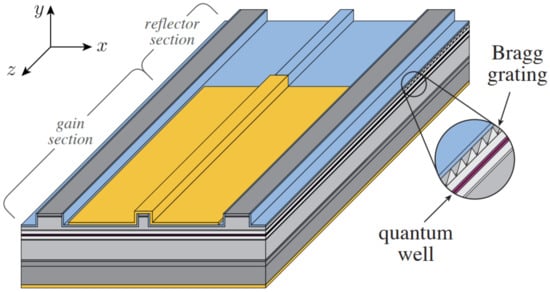
Figure 1. Schematic view of a two-section DBR laser consisting of an electrically biased gain section and a passive Bragg reflector section, exemplifying an edge-emitting multi-section semiconductor laser.

The Langevin forces

$$F_{\mathrm{sp}}(z,t,N)=\left[\begin{array}{c}{F}_{\mathrm{sp}}^{+}(z,t,N)\\ F_{\mathrm{sp}}^{-}(z,t,N)\end{array}\right],$$

model the spontaneous emission into the forward and backward traveling waves and are assumed to have zero mean

$$⟨F_{\mathrm{sp}}⟩=0.$$

Here, $n_{\mathrm{g}}$ is the real-valued group index, $\beta$ is the propagation factor and $\Delta n$ is the static index detuning with respect to the reference modal index. ${\beta }_N$ describes the dependence of the propagation factor on the excess carrier density N, consisting of a real part proportional to $\Delta n_N$ and an imaginary part with g being the modal gain and $\alpha$ the optical losses. ${\kappa }^{\pm }$ are complex coupling coefficients describing a Bragg grating (coupling forward and backward traveling waves) and $\widehat{\mathcal{D}}(z,t)$ is the dispersion operator. The ensemble or temporal average is denoted by $⟨·⟩$. The dependence of $\Delta n_N$, g and $\alpha$ on the optical power ${\parallel \mathsf{\Psi }\parallel }^2$ is due to nonlinear effects like the Kerr effect, gain compression, and two-photon absorption, which affect the stationary states only slightly but can have a significant impact on the dynamic properties.

All quantities entering (2) are obtained by weighting the original quantities entering Maxwell’s equations with the intensity distribution $e^2(x,y)$ of the transverse mode. If we choose the origin of z such that the grating given by a complex dielectric function $\epsilon (x,y,z)$ has the property $\epsilon (x,y,z)=\epsilon (x,y,-z)$, then ${\kappa }^{+}={\kappa }^{-}=\kappa$ holds. Equation (2) has to be solved subject to the usual boundary conditions

$${\mathsf{\Psi }}^{+}(0,t)=r_0{\mathsf{\Psi }}^{-}(0,t)\mathrm{and}{\mathsf{\Psi }}^{-}(L,t)=r_L{\mathrm{e}}^{-2i{\beta }_{0}L}{\mathsf{\Psi }}^{+}(L,t),$$

(4)

with L being the total cavity length and $r_0$ and $r_L$ the complex-valued reflection coefficients at the facets at $z=0$ and $z=L$, respectively. Scattering matrices establish transition conditions on $\mathsf{\Psi }$ at the interfaces between different sections [22,30].

The coupled-wave Equation (2) must be supplemented with an equation for the (excess) carrier density N. Although the theoretical treatment is quite general, we will specifically treat diode lasers in this paper, where the carrier dynamics is governed actually by both electrons and holes. We assume charge neutrality and consider only the excess carriers in the active region with density $N=n-n_0=p-p_0$ (where n and p are the electron and hole densities and $n_0$, $p_0$ are the corresponding equilibrium densities), neglecting any transport and capture effects. Thus, the excess carrier density is assumed to obey the rate equation

$$\frac{\partial N}{\partial t}-\frac{j(z,N)}{qd}+R(z,N)+R_{\mathrm{st}}{(z,N,\parallel \mathsf{\Psi }\parallel }^2)=F_N(z,t,N)$$

(5)

with the rate of spontaneous and non-radiative recombination R and the rate of stimulated recombination

$$R_{\mathrm{st}}=\frac{\mathrm{Re}\left({\mathsf{\Psi }}^{*}·[g-2i\widehat{\mathcal{D}}]\mathsf{\Psi }\right)}{dW\hslash {\omega }_0}$$

(6)

which can be derived by multiplying (2) from the left with $[{\Psi }^{+*},{\Psi }^{-*}]$, the complex conjugate of (2) with $[{\Psi }^{+},{\Psi }^{-}]$ and adding both equations to obtain a balance equation for the electromagnetic energy in differential form (Poynting’s theorem) [30]. Here the dot product means ${\Psi }_1·{\Psi }_2={\Psi }_1^{+}{\Psi }_2^{+}+{\Psi }_1^{-}{\Psi }_2^{-}$ and q is the elementary charge, ℏ the reduced Planck’s constant and d and W are the thickness and width, respectively, of the active region. The current density can be related to the (sectional) applied voltage by means of the Joyce model [32,33]

$$j(z,N)=\frac{U_s-U_{\mathrm{F}}(N)}{W{L}_s{R}_s}$$

(7)

with sectional applied voltage $U_s$, resistance $R_s$, injection current $I_s$, length $L_s$, and the Fermi voltage $U_{\mathrm{F}}$. The carrier-density dependent injection current density given by (7) counteracts longitudinal spatial hole burning, which substantially lowers the degradation of the side mode suppression in strongly coupled DFB lasers compared to a model assuming a constant current density [34]. The frequency modulation response, albeit not topic of the present paper, is also affected as shown in [35].

Dispersion, i.e., the frequency dependence of the dielectric function, enters (2) first via the group index $n_{\mathrm{g}}$ in front of the time derivative resulting from a linearization of the real part of the dielectric function with respect to the frequency $\omega$. Second, the dispersion of the optical gain (and associated refractive index) is described in the time domain by the operator $\widehat{\mathcal{D}}(z,t)$, which can be obtained, e.g., by approximating the gain spectrum by a Lorentzian (or a series of Lorentzians) and a back-transformation into the time domain. This results in auxiliary differential equations for polarization functions [36,37], see Appendix A. Due to the fact, that the spectral width of the gain in semiconductor lasers is much larger than the width of the cavity resonances, $\widehat{\mathcal{D}}(z,t)$ can be expanded again linearly in the frequency domain. In contrast to [36], we neglect here the dependence of the dispersion operator on the carrier density N.

Besides $\mathsf{\Psi }$, we consider N as the only further stochastic variable and spontaneous emission as the only source of noise, neglecting all other noise sources. The theory can be easily extended to include carrier noise as sketched in the Outlook in Section 11. We assume that $\kappa$ does not depend on N, i.e., we exclude gain-coupled lasers, and neglect fluctuations of the shape of the power profile. We neglect the impact of non-lasing side modes on the linewidth of the lasing mode and employ a single-mode approximation. Thus the linewidth rebroadening caused by mode partitioning and poor side-mode suppression, cf.  [38,39], can not be not accounted for.

Regarding the properties of the noise [40], we employ the usual assumptions of ergodicity (ensemble or statistical average equals temporal average) and stationarity (i.e., $⟨\xi (t)\xi (t^{\prime })⟩$ depends only on the time difference $t-t^{\prime }$) of any stochastic variable $\xi$. The fluctuations are assumed to have Gaussian probability distributions and delta-correlated covariance functions in time (Markov approximation) and space, i.e., $⟨\xi (z,t)\zeta (z^{\prime },t^{\prime })⟩=2D_{\xi \zeta }(z)\delta (t-t^{\prime })\delta (z-z^{\prime })$ with $D_{\xi \zeta }$ being called diffusion coefficient. In order to obtain a Lorentzian shape of the optical spectrum around the lasing frequency, some approximations have to be employed which are described in Section 4. The full width at half maximum (FWHM) of the Lorentzian is commonly called intrinsic linewidth. As we consider only spontaneous emission noise, we calculate the quantum limit of the intrinsic linewidth. If non-Markovinan noise is considered, which is beyond of the scope of the paper, the lineshape tends towards a Gaussian in the vicinity of the lasing frequency with a correspondingly larger FWHM [41,42].

3. Equation of the Field Amplitude

Throughout this work, we restrict ourselves to the analysis of the noise at continuous wave (CW) emission, i.e., at steady-state lasing. Therefore, we expand $\mathsf{\Psi }(z,t)$ in terms of the stationary eigenmodes ${\mathsf{\Phi }}_m(z)$ (longitudinal modes),

$$\mathsf{\Psi }(z,t)=\sum _m{f}_m(t){\mathsf{\Phi }}_m(z),$$

(8)

satisfying the equation

$$\left[{\sigma }_z\frac{\partial }{\partial z}+iM\left(z,\overline{N},\overline{{\parallel \mathsf{\Psi }\parallel }^2}\right)+i{\beta }_{\mathcal{D}}(z,{\mathsf{\Omega }}_m)+i\frac{n_{\mathrm{g}}(z)}{c}{\mathsf{\Omega }}_m\right]{\mathsf{\Phi }}_m(z)=0$$

(9)

with

$$\begin{array}{cc}\hfill M\left(z,\overline{N},\overline{{\parallel \mathsf{\Psi }\parallel }^2}\right)& =\left[\begin{array}{cc}\Delta \beta \left(z,\overline{N},\overline{{\parallel \mathsf{\Psi }\parallel }^2}\right)& \kappa (z)\\ \kappa (z)& \Delta \beta \left(z,\overline{N},\overline{{\parallel \mathsf{\Psi }\parallel }^2}\right)\end{array}\right]\equiv \overline{M},\hfill \end{array}$$

(10)

$$\begin{array}{cc}\hfill \Delta \beta \left(z,\overline{N},\overline{{\parallel \mathsf{\Psi }\parallel }^2}\right)& =\beta \left(z,\overline{N},\overline{{\parallel \mathsf{\Psi }\parallel }^2}\right)-{\beta }_0\equiv \overline{\beta }-{\beta }_0=\Delta \overline{\beta }.\hfill \end{array}$$

(11)

Here, $\overline{N}$ and $\overline{{\parallel \mathsf{\Psi }\parallel }^2}$ are the steady-state carrier density and optical power, respectively, at which the operator of the eigenvalue problem (9) is expanded ($\overline{\beta }$, $\overline{M}$ are the corresponding propagation factor and matrix M). The complex eigenvalue ${\mathsf{\Omega }}_m$ describes both, the frequency deviation $\mathrm{Re}({\mathsf{\Omega }}_m)={\omega }_m-{\omega }_0$ (or the wavelength deviation $\Delta {\lambda }_m=\mathrm{Re}({\mathsf{\Omega }}_m){d\lambda /d\omega |}_{{\lambda }_0}$), and the mode damping rate $\mathrm{Im}({\mathsf{\Omega }}_m)$. The dispersion ${\beta }_{\mathcal{D}}(z,{\mathsf{\Omega }}_m)$ is given by the operator $\mathcal{D}(z,t)$ in the frequency domain. Equation (9) has to be solved subject to the boundary conditions

$$\begin{array}{cc}\hfill {\mathsf{\Phi }}_m^{+}(0)& =r_0{\mathsf{\Phi }}_m^{-}(0)\hfill \\ \hfill {\mathsf{\Phi }}_m^{-}(L)& =r_L{\mathrm{e}}^{-2i{\beta }_{0}L}{\mathsf{\Phi }}_m^{+}(L)\hfill \end{array}$$

(12)

following from (4).

In the case of stationary eigenmodes considered here, the two-point boundary value problem (9) together with the boundary conditions (12) is in fact a quasi-linear eigenvalue problem. The point of expansion $\left(\overline{{\parallel \mathsf{\Psi }\parallel }^2},\overline{N}\right)$ of the nonlinear operator must be chosen self-consistently, i.e., it is required to satisfy the conditions (36) and (68) for the (mean) stationary state given below. Furthermore, in the presence of dispersion ${\beta }_{\mathcal{D}}({\mathsf{\Omega }}_m)$, the eigenvalue problem is also nonlinear in the eigenvalue. The problem is similar to the self-consistent field method in electronic structure theory [43] and can be treated in a similar way (e.g., linearization of the optical-power and the frequency dependency of the gain dispersion and fixed-point iteration, where the point of expansion is updated to the most recent stationary state in each step). Alternatively, the system can be directly propagated in the time-domain (as it has been done in Section 10), until convergence to a suitable CW state has been achieved.

Note that different modes (eigensolutions of (9)) fulfill the orthogonality relation

$$({\mathsf{\Phi }}_m,\frac{\partial \beta }{\partial \omega }{\mathsf{\Phi }}_n)=0\mathrm{for}m\ne n$$

(13)

which can be derived by multiplying (9) from the left by $[{\Phi }_n^{-},{\Phi }_n^{+}]$, the corresponding equation for ${\Phi }_n$ by $[{\Phi }_m^{-},{\Phi }_m^{+}]$, integrating along z, using (12) and subtracting both equations. Here the short notation

$$(\mathsf{\Phi },\mathsf{\Psi })={\int }_0^L({\mathsf{\Phi }}^{+}{\mathsf{\Psi }}^{-}+{\mathsf{\Phi }}^{-}{\mathsf{\Psi }}^{+})dz.$$

(14)

denotes an inner product, distinguished from a standard Hilbert space scalar product. At an exceptional point the expansion (8) includes also a generalized eigenmode [10]. For $m=n$, the factor $\partial \beta /\partial \omega$, which can be interpreted as an inverse complex-valued group velocity, is the exact derivative

$$\frac{\partial \beta }{\partial \omega }=\frac{n_{\mathrm{g}}}{c}+\frac{\partial {\beta }_{\mathcal{D}}}{\partial \omega }{|}_{{\mathsf{\Omega }}_m}.$$

(15)

In the general case of $m\ne n$ this holds only approximately:

$$\frac{\partial \beta }{\partial \omega }=\frac{n_{\mathrm{g}}}{c}+\frac{{\beta }_{\mathcal{D}}({\mathsf{\Omega }}_m)-{\beta }_{\mathcal{D}}({\mathsf{\Omega }}_n)}{{\mathsf{\Omega }}_m-{\mathsf{\Omega }}_n}\approx \frac{n_{\mathrm{g}}}{c}+\frac{\partial {\beta }_{\mathcal{D}}}{\partial \omega }{|}_{{\mathsf{\Omega }}_m}.$$

(16)

A system of ordinary differential equations for the amplitudes $f_m(t)$ can be obtained by inserting (8) into (2), using (9), multiplying from left with $[{\mathsf{\Phi }}_n^{-},{\mathsf{\Phi }}_n^{+}]$, and integrating along z. In order to exploit the orthogonality relation (13) with the approximation (16), we have again to expand

$${\beta }_{\mathcal{D}}(\tilde{\omega })-{\beta }_{\mathcal{D}}({\mathsf{\Omega }}_m)=\frac{\partial {\beta }_{\mathcal{D}}}{\partial \omega }{|}_{{\mathsf{\Omega }}_m}(\tilde{\omega }-{\mathsf{\Omega }}_m),$$

(17)

where $\tilde{\omega }=\omega -{\omega }_0$. Note that this is consistent with the slowly varying amplitude approximation. Transforming back into the time domain yields

$$\int \left[{\beta }_{\mathcal{D}}(\tilde{\omega })-{\beta }_{\mathcal{D}}({\mathsf{\Omega }}_m)\right]f_m(\tilde{\omega }){\mathrm{e}}^{i\tilde{\omega }t}d\tilde{\omega }=\left[\widehat{\mathcal{D}}-{\beta }_{\mathcal{D}}({\mathsf{\Omega }}_m)\right]f_m(t)$$

(18)

and

$$\begin{array}{cc}\hfill \frac{\partial {\beta }_{\mathcal{D}}}{\partial \omega }{|}_{{\mathsf{\Omega }}_m}\int (\tilde{\omega }-{\mathsf{\Omega }}_m)f_m(\tilde{\omega }){\mathrm{e}}^{i\tilde{\omega }t}d\tilde{\omega }& =-\frac{\partial {\beta }_{\mathcal{D}}}{\partial \omega }{|}_{{\mathsf{\Omega }}_m}\left[{\mathsf{\Omega }}_m{f}_m(t)+i\frac{\partial }{\partial t}\int f_m(\tilde{\omega }){\mathrm{e}}^{i\tilde{\omega }t}d\tilde{\omega }\right]\hfill \\ & =-\frac{\partial {\beta }_{\mathcal{D}}}{\partial \omega }{|}_{{\mathsf{\Omega }}_m}\left[{\mathsf{\Omega }}_m{f}_m(t)+i\frac{\partial f_m}{\partial t}\right].\hfill \end{array}$$

(19)

Therefore the amplitudes $f_m$ fulfill

$$({\mathsf{\Phi }}_m,\frac{\partial \beta }{\partial \omega }{\mathsf{\Phi }}_m)\frac{\partial f_m}{\partial t}-i{\mathsf{\Omega }}_m({\mathsf{\Phi }}_m,\frac{\partial \beta }{\partial \omega }{\mathsf{\Phi }}_m)f_m+i\sum _n({\mathsf{\Phi }}_m,\Delta M{\mathsf{\Phi }}_n)f_n=({\mathsf{\Phi }}_m,F_{\mathrm{sp}})$$

(20)

with

$$\Delta M=M-\overline{M}=(\beta -\overline{\beta })\left[\begin{array}{cc}1& 0\\ 0& 1\end{array}\right].$$

(21)

In what follows, we employ the single mode approximation and drop the subscript m. Then (20) becomes a single differential equation for the complex-valued amplitude f of the lasing mode

$$\frac{\partial f}{\partial t}-i\mathsf{\Omega }f+i\frac{(\mathsf{\Phi },\Delta M\mathsf{\Phi })}{(\mathsf{\Phi },\frac{\partial \beta }{\partial \omega }\mathsf{\Phi })}f=F_f.$$

(22)

The new Langevin noise source entering (22) is given by

$$F_f=\frac{(\mathsf{\Phi },F_{\mathrm{sp}})}{(\mathsf{\Phi },\frac{\partial \beta }{\partial \omega }\mathsf{\Phi })}.$$

(23)

For an analysis above threshold, it is beneficial to derive equations for the modulus $\left|f\right|$ and the phase $\phi$ of f, because the fluctuations of $\left|f\right|$ are damped but those of $\phi$ are not. For the modulus squared ${\left|f\right|}^2$ (called intensity in the rest of the paper) it follows

$$\frac{{\partial \left|f\right|}^2}{\partial t}+{2\mathrm{Im}(\mathsf{\Omega })\left|f\right|}^2-2\mathrm{Im}\frac{(\mathsf{\Phi },\Delta M\mathsf{\Phi })}{(\mathsf{\Phi },\frac{\partial \beta }{\partial \omega }\mathsf{\Phi })}{\left|f\right|}^2=2\mathrm{Re}(F_f{f}^{*}).$$

(24)

An equation for the phase can be determined from

$$\mathrm{Im}\left(\frac{\partial f}{\partial t}{f}^{*}\right)-{\mathrm{Re}(\mathsf{\Omega })\left|f\right|}^2+\mathrm{Re}\frac{(\mathsf{\Phi },\Delta M\mathsf{\Phi })}{(\mathsf{\Phi },\frac{\partial \beta }{\partial \omega }\mathsf{\Phi })}{\left|f\right|}^2=\mathrm{Im}(F_f{f}^{*})$$

(25)

and

$$\frac{\partial f}{\partial t}={\mathrm{e}}^{i\phi }\frac{\partial \left|f\right|}{\partial t}+if\frac{\partial \phi }{\partial t}⟹\mathrm{Im}\left(\frac{\partial f}{\partial t}{f}^{*}\right)={\left|f\right|}^2\frac{\partial \phi }{\partial t}.$$

(26)

The stochastic term on the right-hand side of (24) describes intensity noise, which does not have a vanishing expectation value anymore: $⟨F_f{f}^{*}⟩\ne 0$. It is therefore convenient to rewrite the term by distilling out the expectation value and introducing two new real-valued Langevin forces $F_{{\left|f\right|}^2}$ and $F_{\phi }$ with zero mean as

$$2F_f{f}^{*}=2⟨F_f{f}^{*}⟩+F_{{\left|f\right|}^2}+2i{\left|f\right|}^2{F}_{\phi }.$$

(27)

It will be shown below that $⟨F_f{f}^{*}⟩$ is real-valued, see (66). Then, the final equations for the modulus squared and phase of f read

$$\frac{{\partial \left|f\right|}^2}{\partial t}=-{2\mathrm{Im}(\mathsf{\Omega })\left|f\right|}^2+2\mathrm{Im}\frac{(\mathsf{\Phi },\Delta M\mathsf{\Phi })}{(\mathsf{\Phi },\frac{\partial \beta }{\partial \omega }\mathsf{\Phi })}{\left|f\right|}^2+2⟨F_f{f}^{*}⟩+F_{{\left|f\right|}^2}$$

(28)

and

$$\frac{\partial \phi }{\partial t}=\mathrm{Re}(\mathsf{\Omega })-\mathrm{Re}\frac{(\mathsf{\Phi },\Delta M\mathsf{\Phi })}{(\mathsf{\Phi },\frac{\partial \beta }{\partial \omega }\mathsf{\Phi })}+F_{\phi }.$$

(29)

Now we consider small fluctuations

$$\begin{array}{cc}\hfill N(z,t)& =⟨N(z)⟩+\delta N(z,t),\hfill \end{array}$$

(30)

$$\begin{array}{cc}\hfill \phi (t)& =⟨\phi (t)⟩+\delta \phi (t),\hfill \end{array}$$

(31)

$$\begin{array}{cc}\hfill {\left|f(t)\right|}^2& ={⟨\left|f\right|}^2{⟩+\delta \left|f(t)\right|}^2\hfill \end{array}$$

(32)

and expand

$$\beta ={\beta (⟨N⟩,⟨|f|}^2⟩)+\frac{\partial \beta }{\partial N}{|}_{⟨N⟩,⟨|f{|}^2⟩}\delta N+\frac{\partial \beta }{{\partial \left|f\right|}^2}{|}_{⟨N⟩,⟨|f{|}^2⟩}\delta {\left|f\right|}^2$$

(33)

around the mean values

$$\begin{array}{cc}\hfill ⟨N(z)⟩& =\overline{N}(z),\hfill \\ \hfill ⟨\phi (t)⟩& =\mathrm{Re}(\mathsf{\Omega })t.\hfill \end{array}$$

(34)

The mean intensity $⟨|f{|}^2⟩$ is required to satisfy

$${\mathrm{Im}(\mathsf{\Omega })⟨\left|f\right|}^2⟩=⟨F_f{f}^{*}⟩.$$

(35)

Due to the extreme smallness of the spontaneous emission $⟨F_f{f}^{*}⟩$ going into the lasing mode, (35) can be replaced by

$$\mathrm{Im}(\mathsf{\Omega })=0$$

(36)

above threshold ${(⟨|f|}^2⟩0)$, which will be exploited in what follows (i.e., $\mathsf{\Omega }=\mathrm{Re}(\mathsf{\Omega })$). The intensity and phase fluctuations fulfill the equations

$$\frac{{\partial \delta \left|f\right|}^2}{\partial t}=2\mathrm{Im}\frac{(\mathsf{\Phi },\frac{\partial \beta }{\partial N}\delta N\mathsf{\Phi })+(\mathsf{\Phi },\frac{\partial \beta }{{\partial \left|f\right|}^2}\mathsf{\Phi })\delta {\left|f\right|}^2}{(\mathsf{\Phi },\frac{\partial \beta }{\partial \omega }\mathsf{\Phi })}{⟨\left|f\right|}^2⟩+F_{{\left|f\right|}^2}$$

(37)

and

$$\frac{\partial \delta \phi }{\partial t}=-\mathrm{Re}\frac{(\mathsf{\Phi },\frac{\partial \beta }{\partial N}\delta N\mathsf{\Phi })+(\mathsf{\Phi },\frac{\partial \beta }{{\partial \left|f\right|}^2}\mathsf{\Phi })\delta {\left|f\right|}^2}{(\mathsf{\Phi },\frac{\partial \beta }{\partial \omega }\mathsf{\Phi })}+F_{\phi },$$

(38)

which are the basis for the derivation of the linewidth formula in the following sections.

4. Lorentzian Line Shape

The power spectral density (PSD) of the optical field at $z=0$ can be calculated utilizing the Wiener–Khinchin theorem as [44]

$$S_E(\omega )=\int \int {\int }_{-\infty }^{+\infty }⟨E^{*}(x,y,0,t)E(x,y,0,t+\tau )⟩{\mathrm{e}}^{-i\omega \tau }d\tau dxdy$$

(39)

with

$$⟨E^{*}(x,y,0,t)E(x,y,0,t+\tau )⟩=\frac{1-|r_0{|}^2}{2{\epsilon }_{0}cn}{e}^2(x,y)⟨f^{*}(t)f(t+\tau )⟩{\left|{\mathsf{\Phi }}^{-}(0)\right|}^2{\mathrm{e}}^{i{\omega }_0\tau }+\mathrm{c}.\mathrm{c}.$$

(40)

We do not address here technical issues regarding the non-existence of Fourier integrals of fluctuating quantities here and refer to the discussion in [44]. Hence we have to calculate the PSD

$$S_f(\omega )={\int }_{-\infty }^{+\infty }⟨f^{*}(t)f(t+\tau )⟩{\mathrm{e}}^{-i(\omega -{\omega }_0)\tau }d\tau$$

(41)

with

$$⟨f^{*}(t)f(t+\tau )⟩=⟨\left|f(t)\right|\left|f(t+\tau )\right|{\mathrm{e}}^{i[\phi (t+\tau )-\phi (t)]}⟩.$$

(42)

Now we employ here a first approximation: We neglect in (42) the intensity fluctuations because above threshold they are damped, in contrast to the phase fluctuations, which can been seen by comparing (37) and (38), see the discussion in [45]. Therefore, we obtain

$$⟨f^{*}(t)f(t+\tau )⟩\approx {⟨\left|f\right|}^2⟩⟨{\mathrm{e}}^{i{\Delta }_{\tau }\phi }⟩{\mathrm{e}}^{i\mathsf{\Omega }\tau }$$

(43)

with

$${\Delta }_{\tau }\phi =\delta \phi (t+\tau )-\delta \phi (t)$$

(44)

and $\mathsf{\Omega }=\mathrm{Re}(\mathsf{\Omega })$. The random variable ${\Delta }_{\tau }\phi$ is assumed to be Gaussian distributed [46], such that it holds

$$⟨{\mathrm{e}}^{i{\Delta }_{\tau }\phi }⟩=\frac{1}{\sqrt{2\pi \mathrm{Var}({\Delta }_{\tau }\phi )}}{\int }_{-\infty }^{\infty }{\mathrm{e}}^{-\frac{{({\Delta }_{\tau }\phi )}^2}{2\mathrm{Var}({\Delta }_{\tau }\phi )}}{\mathrm{e}}^{i{\Delta }_{\tau }\phi }d{\Delta }_{\tau }\phi ={\mathrm{e}}^{-\frac{1}{2}\mathrm{Var}({\Delta }_{\tau }\phi )}.$$

(45)

The variance of the phase fluctuations is

$$\begin{array}{cc}\hfill \mathrm{Var}({\Delta }_{\tau }\phi )& =⟨{\left({\Delta }_{\tau }\phi -⟨{\Delta }_{\tau }\phi ⟩\right)}^2⟩\hfill \\ & =⟨{({\Delta }_{\tau }\phi )}^2⟩\hfill \\ & =⟨{\left(\delta \phi (t+\tau )\right)}^2⟩-2⟨\delta \phi (t)\delta \phi (t+\tau )⟩+⟨{\left(\delta \phi (t)\right)}^2⟩\hfill \\ & =2\left[⟨{\left(\delta \phi (0)\right)}^2⟩-⟨\delta \phi (0)\delta \phi (\tau )⟩\right],\hfill \end{array}$$

(46)

where we exploited $⟨{\Delta }_{\tau }\phi ⟩=0$ and the stationarity property. We introduce the PSD of phase fluctuations which is even in the frequency ($S_{\delta \phi }\left(\tilde{\omega }\right)=S_{\delta \phi }(-\tilde{\omega })$)

$$S_{\delta \phi }(\tilde{\omega })={\int }_{-\infty }^{+\infty }⟨\delta \phi (t)\delta \phi (t+\tau )⟩{\mathrm{e}}^{-i\tilde{\omega }\tau }d\tau$$

(47)

and the PSD of optical frequency fluctuations $\delta \omega (\tilde{\omega })=i\tilde{\omega }\delta \phi (\tilde{\omega })$

$$S_{\delta \omega }(\tilde{\omega })={\int }_{-\infty }^{+\infty }⟨\delta \omega (t)\delta \omega (t+\tau )⟩{\mathrm{e}}^{-i\tilde{\omega }\tau }d\tau ={\tilde{\omega }}^2{S}_{\delta \phi }(\tilde{\omega }).$$

(48)

With these spectral densities, the variance of the phase fluctuations can be written as

$$\begin{array}{cc}\hfill \mathrm{Var}({\Delta }_{\tau }\phi )& =\frac{1}{\pi }{\int }_{-\infty }^{\infty }{S}_{\delta \phi }(\tilde{\omega })\left(1-{\mathrm{e}}^{i\tilde{\omega }\tau }\right)d\tilde{\omega }\hfill \\ & =\frac{1}{\pi }{\int }_{-\infty }^{\infty }{S}_{\delta \phi }(\tilde{\omega })\left(2{\sin }^2\left(\frac{\tilde{\omega }\tau }{2}\right)-i\sin \left(\tilde{\omega }\tau \right)\right)d\tilde{\omega }\hfill \\ & =\frac{2}{\pi }{\int }_{-\infty }^{\infty }{S}_{\delta \phi }(\tilde{\omega }){\sin }^2\left(\frac{\tilde{\omega }\tau }{2}\right)d\tilde{\omega }\hfill \\ & =\frac{{\tau }^2}{2\pi }{\int }_{-\infty }^{\infty }{S}_{\delta \omega }(\tilde{\omega }){\left(\frac{\sin \left(\frac{\tilde{\omega }\tau }{2}\right)}{\frac{\tilde{\omega }\tau }{2}}\right)}^{2}d\tilde{\omega }.\hfill \end{array}$$

(49)

We carry out a second approximation by noting that the function ${\sin }^2\left(\frac{\tilde{\omega }\tau }{2}\right)/{(\frac{\tilde{\omega }\tau }{2})}^2$ peaks strongly at $\tilde{\omega }=0$ for large $\left|\tau \right|$, and obtain

$$\mathrm{Var}({\Delta }_{\tau }\phi )\approx \frac{\left|\tau \right|}{\pi }{S}_{\delta \omega }(0){\int }_{-\infty }^{\infty }\frac{{\sin }^{2}x}{x^2}dx=\left|\tau \right|S_{\delta \omega }(0).$$

(50)

In this step, we have recovered a central property of Brownian motion, as we can observe that the root mean square displacement of the phase fluctuation grows as $\propto \sqrt{\left|\tau \right|}$. Inserting (50) into (45) and, finally, the result into (43) yields

$$⟨f^{*}(t)f(t+\tau )⟩\approx {⟨\left|f\right|}^2⟩{\mathrm{e}}^{-\frac{1}{2}{S}_{\delta \omega }(0)\left|\tau \right|}{\mathrm{e}}^{i\mathsf{\Omega }\tau }$$

(51)

and

$$\begin{array}{cc}\hfill S_f(\omega )& \approx {⟨\left|f\right|}^2⟩{\int }_{-\infty }^{+\infty }{\mathrm{e}}^{-\frac{1}{2}{S}_{\delta \omega }(0)\left|\tau \right|+i({\omega }_0+\mathsf{\Omega }-\omega )\tau }d\tau \hfill \\ & ={⟨\left|f\right|}^2⟩\frac{S_{\delta \omega }(0)}{{\left(\omega -({\omega }_0+\mathsf{\Omega })\right)}^2+{\left(\frac{S_{\delta \omega }(0)}{2}\right)}^2}.\hfill \end{array}$$

(52)

This is a Lorentzian centered at $\omega ={\omega }_0+\mathsf{\Omega }$ with the FWHM

$$\Delta \omega =S_{\delta \omega }(0)$$

(53)

given by the PSD of the optical frequency fluctuations taken at zero Fourier frequency.

In the following sections of this paper, we will focus on the static white noise limit, where the frequency noise PSD $S_{\delta \omega }(\omega )$ is effectively approximated by a constant, such that the second approximation carried out on the step from (49) to (50) becomes in fact redundant.

5. Correlation Functions

The correlation function of the spontaneous emission noise $F_f$ defined in (23) is

$$⟨F_f^{*}(t)F_f(t^{\prime })⟩=\frac{⟨({\mathsf{\Phi }}^{*},F_{\mathrm{sp}}^{*}(z,t))(\mathsf{\Phi },F_{\mathrm{sp}}(z^{\prime },t^{\prime }))⟩}{{\left|(\mathsf{\Phi },\frac{\partial \beta }{\partial \omega }\mathsf{\Phi })\right|}^2}.$$

(54)

The numerator reads

$$\begin{array}{c}⟨({\mathsf{\Phi }}^{*},F_{\mathrm{sp}}^{*}(z,t))(\mathsf{\Phi },F_{\mathrm{sp}}(z^{\prime },t^{\prime }))⟩\hfill \\ ={\int }_0^L{\int }_0^L⟨\left[{\mathsf{\Phi }}^{+*}{F}_{\mathrm{sp}}^{-*}(z,t)+{\mathsf{\Phi }}^{-*}{F}_{\mathrm{sp}}^{+*}(z,t)\right]\left[{\mathsf{\Phi }}^{+}{F}_{\mathrm{sp}}^{-}(z^{\prime },t^{\prime })+{\mathsf{\Phi }}^{-}{F}_{\mathrm{sp}}^{+}(z^{\prime },t^{\prime })\right]⟩dzd{z}^{\prime }\hfill \\ ={\int }_0^L{\int }_0^L\left[|{\mathsf{\Phi }}^{+}{|}^2⟨F_{\mathrm{sp}}^{-*}(z,t)F_{\mathrm{sp}}^{-}(z^{\prime },t^{\prime })⟩+{\left|{\mathsf{\Phi }}^{-}\right|}^2⟨F_{\mathrm{sp}}^{+*}(z,t)F_{\mathrm{sp}}^{+}(z^{\prime },t^{\prime })⟩\right]dzd{z}^{\prime }\hfill \\ =2{\int }_0^L{\parallel \mathsf{\Phi }(z)\parallel }^2{D}_{\mathrm{sp}}(z)dz\delta (t-t^{\prime })\hfill \end{array}$$

(55)

with

$${\parallel \mathsf{\Phi }\parallel }^2=|{\mathsf{\Phi }}^{+}{|}^2+{\left|{\mathsf{\Phi }}^{-}\right|}^2$$

(56)

taking into account the noise covariance functions [25,26,27] for index and absorption coupling

$$\begin{array}{cc}\hfill ⟨F_{\mathrm{sp}}^{\pm *}(z,t)F_{\mathrm{sp}}^{\pm }(z^{\prime },t^{\prime })⟩& =2D_{\mathrm{sp}}(z)\delta (t-t^{\prime })\delta (z-z^{\prime }),\hfill \\ \hfill ⟨F_{\mathrm{sp}}^{\mp *}(z,t)F_{\mathrm{sp}}^{\pm }(z^{\prime },t^{\prime })⟩& =0,\hfill \\ \hfill ⟨F_{\mathrm{sp}}^{\pm }(z,t)F_{\mathrm{sp}}^{\pm }(z^{\prime },t^{\prime })⟩& =0,\hfill \\ \hfill ⟨F_{\mathrm{sp}}^{\mp }(z,t)F_{\mathrm{sp}}^{\pm }(z^{\prime },t^{\prime })⟩& =0\hfill \end{array}$$

(57)

with

$$2D_{\mathrm{sp}}{(z,N,\parallel \mathsf{\Psi }\parallel }^2)=\hslash {\omega }_0{n}_{\mathrm{sp}}{(N)g(z,N,\parallel \mathsf{\Psi }\parallel }^2),$$

(58)

where $n_{\mathrm{sp}}$ is the population inversion factor (a Bose–Einstein distribution function multiplied by $-1$). The correlation functions for gain-coupling can be found in [47].

Since $\mathsf{\Psi }$ has the unit $\sqrt{\mathrm{W}}$, $D_{\mathrm{sp}}$ must have the unit Ws/m as it is. The diffusion coefficient $D_{f^{*}f}$ defined by

$$⟨F_f^{*}(t)F_f(t^{\prime })⟩=2D_{f^{*}f}\delta (t-t^{\prime }).$$

(59)

is therefore

$$D_{f^{*}f}=D_{f^{*}f}{(N,\parallel \mathsf{\Psi }\parallel }^2)=\frac{{\int }_0^L{\parallel \mathsf{\Phi }(z)\parallel }^2{D}_{\mathrm{sp}}{(z,N,\parallel \mathsf{\Psi }\parallel }^2)dz}{{\left|(\mathsf{\Phi },\frac{\partial \beta }{\partial \omega }\mathsf{\Phi })\right|}^2}.$$

(60)

The correlation functions of the Langevin forces entering (37) and (38) read

$$\begin{array}{cc}\hfill ⟨F_{{\left|f\right|}^2}(t)F_{{\left|f\right|}^2}(t^{\prime })⟩& =2D_{{\left|f\right|}^2{\left|f\right|}^2}\delta (t-t^{\prime })=4D_{f^{*}f}{⟨\left|f\right|}^2⟩\delta (t-t^{\prime }),\hfill \end{array}$$

(61)

$$\begin{array}{cc}\hfill ⟨F_{\phi }(t)F_{\phi }(t^{\prime })⟩& =2D_{\phi \phi }\delta (t-t^{\prime })=\frac{D_{f^{*}f}}{⟨|f{|}^2⟩}\delta (t-t^{\prime }),\hfill \end{array}$$

(62)

$$\begin{array}{cc}\hfill ⟨F_{{\left|f\right|}^2}(t)F_{\phi }(t^{\prime })⟩& =2D_{{\left|f\right|}^2\phi }\delta (t-t^{\prime })=0,\hfill \end{array}$$

(63)

which can be derived using the transformation rules for the diffusion coefficients [23]

$$\begin{array}{cc}\hfill D_{{\left|f\right|}^2{\left|f\right|}^2}& =\left(\frac{{\partial \left|f\right|}^2}{\partial f}\frac{{\partial \left|f\right|}^2}{\partial f^{*}}+\frac{{\partial \left|f\right|}^2}{\partial f^{*}}\frac{{\partial \left|f\right|}^2}{\partial f}\right)D_{f^{*}f},\hfill \\ \hfill D_{\phi \phi }& =\left(\frac{\partial \phi }{\partial f}\frac{\partial \phi }{\partial f^{*}}+\frac{\partial \phi }{\partial f^{*}}\frac{\partial \phi }{\partial f}\right)D_{f^{*}f},\hfill \\ \hfill D_{{\left|f\right|}^2\phi }& =\left(\frac{{\partial \left|f\right|}^2}{\partial f}\frac{\partial \phi }{\partial f^{*}}+\frac{{\partial \left|f\right|}^2}{\partial f^{*}}\frac{\partial \phi }{\partial f}\right)D_{f^{*}f},\hfill \end{array}$$

(64)

and the relations ${\left|f\right|}^2=f^{*}f$ and $\phi =-\frac{i}{2}\ln (f/f^{*})$. Following [48], the ensemble average defined in (27) can be obtained using the formal solution of (22) in the form of

$$f\left(t\right)=f\left(t-\Delta t\right)+{\int }_{t-\Delta t}^t\frac{\partial f^{*}(t^{\prime })}{\partial t^{\prime }}d{t}^{\prime },$$

(65)

where the time step $0<\Delta t\ll {\gamma }_R^{-1}$ is assumed to be short in comparison to the (inverse) relaxation rate ${\gamma }_R=\mathrm{Im}\left(\mathsf{\Omega }-\left(\mathsf{\Phi },\Delta M\mathsf{\Phi }\right)/\left(\mathsf{\Phi },{\partial }_{\omega }\beta \mathsf{\Phi }\right)\right)$. Substituting (65) into $⟨F_f\left(t\right)f^{*}\left(t\right)⟩$ yields

$$\begin{array}{cc}\hfill ⟨F_f\left(t\right)f^{*}\left(t\right)⟩& =⟨F_f\left(t\right)f^{*}\left(t-\Delta t\right)⟩+{\int }_{t-\Delta t}^t⟨F_f\left(t\right)\frac{\partial f^{*}(t^{\prime })}{\partial t^{\prime }}⟩d{t}^{\prime }\hfill \\ & =⟨F_f\left(t\right)⟩⟨f^{*}\left(t-\Delta t\right)⟩-i{\int }_{t-\Delta t}^t{\left(\mathsf{\Omega }-\frac{\left(\mathsf{\Phi },\Delta M\mathsf{\Phi }\right)}{\left(\mathsf{\Phi },\partial \beta /\partial \omega \mathsf{\Phi }\right)}\right)}^{*}⟨F_f\left(t\right)f^{*}\left(t^{\prime }\right)⟩d{t}^{\prime }\hfill \\ & \phantom{=}+{\int }_{t-\Delta t}^t⟨F_f\left(t\right)F_f^{*}\left(t^{\prime }\right)⟩d{t}^{\prime },\hfill \end{array}$$

where we have used (22) in the second step. The first term vanishes because of causality, since the fluctuations of $f^{*}\left(t-\Delta t\right)$ are not correlated with the future noise $F_f\left(t\right)$. Consequently, the correlation function factorizes and results in zero due to the zero-mean property of the Langevin force. The second term can be dropped since it is non-zero only over a set of measure zero (i.e., at $t=t^{\prime }$). Finally, we obtain with (59)

$$⟨F_f\left(t\right)f^{*}\left(t\right)⟩={\int }_{t-\Delta t}^t⟨F_f\left(t\right)F_f^{*}\left(t^{\prime }\right)⟩d{t}^{\prime }=D_{f^{*}f},$$

(66)

where a factor 2 is canceled by 1/2 encountered in integrating only half of the $\delta$-function.

6. Effective Linewidth Enhancement Factor

Using the ansatz (8), we can approximate the rate of stimulated emission (6) as

$$R_{\mathrm{st}}=\frac{g+2\mathrm{Im}\left({\beta }_{\mathcal{D}}(\mathsf{\Omega })\right)}{dW\hslash {\omega }_0}{\left|f\right|}^2{\parallel \mathsf{\Phi }\parallel }^2.$$

(67)

The stationary mean value of the carrier density and its fluctuations satisfy

$$\frac{j(⟨N⟩)}{ed}=R(⟨N⟩)+\frac{{g(⟨N⟩,⟨|f|}^2{⟩\parallel \mathsf{\Phi }\parallel }^2)+2\mathrm{Im}\left({\beta }_{\mathcal{D}}(\mathsf{\Omega })\right)}{dW\hslash {\omega }_0}{⟨\left|f\right|}^2{⟩\parallel \mathsf{\Phi }\parallel }^2$$

(68)

and

$$\frac{\partial \delta N}{\partial t}+\frac{\delta N}{{\tau }_{\mathrm{d}}}+\frac{\partial R_{\mathrm{st}}}{{\partial \left|f\right|}^2}\delta {\left|f\right|}^2=F_N,$$

(69)

respectively, with the inverse differential carrier lifetime (taken at $⟨N⟩$ and $⟨|f{|}^2⟩$)

$$\frac{1}{{\tau }_{\mathrm{d}}}=-\frac{1}{qd}\frac{\partial j}{\partial N}+\frac{\partial R}{\partial N}+\frac{\partial R_{\mathrm{st}}}{\partial N}.$$

(70)

The FWHM of the Lorentzian line shape is given by the spectral density of the frequency fluctuations at zero Fourier frequency, cf. (53). This is equivalent to setting the time derivatives of the fluctuations equal to zero (static limit)

$$\frac{{\partial \delta \left|f\right|}^2}{\partial t}=0$$

(71)

and

$$\frac{\partial \delta N}{\partial t}=0.$$

(72)

Furthermore, we omit carrier noise ($F_N=0$), considering only spontaneous emission noise as mentioned in Section 2. With these approximations, the carrier density fluctuations are directly related to the intensity fluctuations by

$$\delta N=-{\tau }_{\mathrm{d}}\frac{\partial R_{\mathrm{st}}}{{\partial \left|f\right|}^2}\delta {\left|f\right|}^2.$$

(73)

We substitute (73) into (37) and obtain

$${\delta \left|f\right|}^2=\frac{F_{{\left|f\right|}^2}}{{2⟨\left|f\right|}^2⟩\mathrm{Im}(h_{\alpha })}$$

(74)

with

$$h_{\alpha }=\frac{(\mathsf{\Phi },{\tau }_{\mathrm{d}}\frac{\partial \beta }{\partial N}\frac{\partial R_{\mathrm{st}}}{{\partial \left|f\right|}^2}\mathsf{\Phi })-(\mathsf{\Phi },\frac{\partial \beta }{{\partial \left|f\right|}^2}\mathsf{\Phi })}{(\mathsf{\Phi },\frac{\partial \beta }{\partial \omega }\mathsf{\Phi })}.$$

(75)

Inserting (74) back into (73) yields

$$\delta N=-{\tau }_{\mathrm{d}}\frac{\partial R_{\mathrm{st}}}{{\partial \left|f\right|}^2}\frac{F_{{\left|f\right|}^2}}{{2⟨\left|f\right|}^2⟩\mathrm{Im}(h_{\alpha })}.$$

(76)

Finally, substituting (76) into (38) results in

$$\frac{\partial \delta \phi }{\partial t}=\frac{F_{{\left|f\right|}^2}}{2⟨|f{|}^2⟩}\frac{\mathrm{Re}(h_{\alpha })}{\mathrm{Im}(h_{\alpha })}+F_{\phi },$$

(77)

which can be considered as a defining equation for the so-called effective Henry’s $\alpha$-factor

$${\alpha }_{\mathrm{H},\mathrm{eff}}=-\frac{\mathrm{Re}(h_{\alpha })}{\mathrm{Im}(h_{\alpha })}.$$

(78)

If ${\alpha }_{\mathrm{H},\mathrm{eff}}\ne 0$, the Langevin force resulting in fluctuations of the intensity leads also to fluctuations of the phase. By virtue of the different integrals in the numerator and denominator of (75), the carrier dependence of the propagation factor, nonlinear gain (gain compression), absorption (two-photon absorption) and index (Kerr effect) as well as gain dispersion are accounted for. The impact of longitudinal spatial hole burning and multi-section cavity structures (e.g., including Bragg gratings, passive sections or external cavities) is also correctly described. If all of these additional effects are neglected, for a Fabry–Pérot (FP) laser the $\alpha$-factor is recovered

$${\alpha }_{\mathrm{H}}=-\frac{\mathrm{Re}\left(\frac{\partial \beta }{\partial N}\right)}{\mathrm{Im}\left(\frac{\partial \beta }{\partial N}\right)}=-\frac{4\pi }{{\lambda }_0}\frac{\frac{\partial \Delta n_N}{\partial N}}{\frac{\partial g}{\partial N}-\frac{\partial \alpha }{\partial N}}.$$

(79)

The second equality is obtained using (3c). The minus sign in (78), resulting in a corresponding minus sign in (79), has been chosen in agreement with the usual convention ensuring positive values of ${\alpha }_{\mathrm{H}}$ around the gain peak [49]. The derivative $\partial \alpha /\partial N$ of the modal absorption in (79) is often neglected, cf. [49]. One should keep in mind that ${\alpha }_{\mathrm{H}}$ is not a constant but depends on the carrier density (and the wavelength) because modal index and gain vary differently with carrier density.

7. Spectral Linewidth

Collecting the results of the previous sections, we can now calculate the spectral linewidth. Rewriting (53) as

$$\Delta \omega ={\int }_{-\infty }^{+\infty }⟨\frac{\partial \delta \phi (t)}{\partial t}\frac{\partial \delta \phi (t+\tau )}{\partial t}⟩d\tau$$

(80)

and inserting the equation of the phase fluctuations (77), we obtain

$$\Delta \omega =\frac{{\alpha }_{\mathrm{H},\mathrm{eff}}^2}{{4⟨\left|f\right|}^2{⟩}^2}{\int }_{-\infty }^{\infty }⟨F_{{\left|f\right|}^2}(t)F_{{\left|f\right|}^2}(t+\tau )⟩d\tau +{\int }_{-\infty }^{\infty }⟨F_{\phi }(t)F_{\phi }(t+\tau )⟩d\tau ,$$

(81)

where we have taken (63) into account. Inserting (61) and (62) results in the remarkably simple expression for the spectral linewidth

$$\Delta \nu =\frac{\Delta \omega }{2\pi }=\frac{D_{f^{*}f}}{2\pi ⟨|f{|}^2⟩}\left(1+{\alpha }_{\mathrm{H},\mathrm{eff}}^2\right).$$

(82)

In the following, we will rewrite this expression in terms of the intra-cavity photon number

$$I_{\mathrm{ph}}=\frac{1}{\hslash {\omega }_0}{\int }_0^{L}P\mathrm{Re}\left(\frac{\partial \beta }{\partial \omega }\right)dz=\frac{P_0}{\hslash {\omega }_0}\frac{{\int }_0^L{\parallel \mathsf{\Phi }\parallel }^2\mathrm{Re}\left(\frac{\partial \beta }{\partial \omega }\right)dz}{(1-|r_0{|}^2)|{\mathsf{\Phi }}^{-}{(0)|}^2}$$

(83)

where

$$P(z)={⟨\left|f\right|}^2{⟩\parallel \mathsf{\Phi }(z)\parallel }^2$$

(84)

is the stationary optical power inside the cavity and

$$P_0=(1-|r_0{|}^2{)⟨|f|}^2⟩|{\mathsf{\Phi }}^{-}{(0)|}^2$$

(85)

is the outcoupled power at $z=0$. Moreover, we define the rate of spontaneous emission into the lasing mode

$$R_{\mathrm{sp}}=\frac{{\int }_0^L{\parallel \mathsf{\Phi }\parallel }^2{n}_{\mathrm{sp}}gdz}{{\int }_0^L{\parallel \mathsf{\Phi }\parallel }^2\mathrm{Re}\left(\frac{\partial \beta }{\partial \omega }\right)dz}$$

(86)

and the longitudinal excess factor of spontaneous emission

$$K=\frac{{\left({\int }_0^L{\parallel \mathsf{\Phi }\parallel }^2\mathrm{Re}\left(\frac{\partial \beta }{\partial \omega }\right)dz\right)}^2}{{\left|(\mathsf{\Phi },\frac{\partial \beta }{\partial \omega }\mathsf{\Phi })\right|}^2}.$$

(87)

Now, (82) can be written as

$$\Delta \nu =\frac{K{R}_{\mathrm{sp}}}{4\pi I_{\mathrm{ph}}}\left(1+{\alpha }_{\mathrm{H},\mathrm{eff}}^2\right)$$

(88)

which is the standard form found in the literature [14,46].

The mode profile $\mathsf{\Phi }(z)$ entering (83), (86), and (87) is obtained by solving (9), (36) and (68) self-consistently above threshold. Thus, $\mathsf{\Phi }$ is a mode of the active cavity affected by spatial hole burning. The expression for the K-factor generalizes the one given in [10] for non-uniform and complex-valued group velocity ${(\partial \beta /\partial \omega )}^{-1}$ and is in basic correspondence with [14,50,51], but fundamentally different from the modified K-factor introduced in [52].

At an exceptional point, the mode is orthogonal to itself, i.e., $(\mathsf{\Phi },\frac{\partial \beta }{\partial \omega }\mathsf{\Phi })=0$, and the K-factor approaches infinity. However, one has to keep in mind that at an exceptional point the single-mode approximation used here fails. Instead, for the description of the dynamics in the vicinity of such a point one has use at least one eigenmode and the corresponding generalized eigenmode [10].

8. Impact of a Passive Section, Chirp Reduction Factor and the Fabry–Pérot Case

In this section, we apply the general theory developed above to special configurations that allow for further simplifications (i.e., neglect of spatial hole burning, nonlinear gain and index as well gain dispersion). Thereby, it is shown that the general framework entails some well-established formulas from the literature as special cases.

8.1. Linewidth of a Laser Consisting of a Gain Chip Subject to Feedback from an External Cavity

We consider a laser consisting of one active section for $z\in [0,l]$ with length l and an arbitrary number of passive sections (including an external cavity) for $z\in [l,L]$ with total length $L-l$. The active section is of the Fabry–Pérot (FP) type having no Bragg grating ($\kappa =0$ for $z\in [0,l])$. The passive sections may contain Bragg gratings but no excess carriers ($N=0$, $\partial \beta /\partial N=0$, $D_{\mathrm{sp}}=0$, $R_{\mathrm{st}}=0$ for $z\in [l,L]$). The reference plane is located just inside the active section so that a possible finite reflectivity at the interface between active and passive sections belongs to the passive sections. Furthermore, we neglect spatial hole burning (i.e., $\partial N/\partial z=0$), nonlinear gain and index ($\partial \beta /{\partial \left|f\right|}^2=0$, $\partial R_{\mathrm{st}}/{\partial \left|f\right|}^2=R_{\mathrm{st}}/{\left|f\right|}^2$) and gain dispersion (${\beta }_{\mathcal{D}}=0$, $\partial \beta /\partial \omega =n_{\mathrm{g}}/c$). See Figure 2 for an illustration of the device.

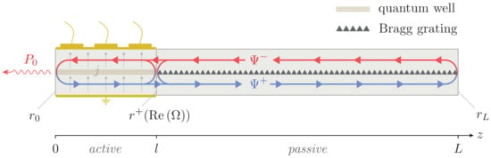
Figure 2. Schematic illustration of a two-section DBR laser featuring an active gain section and a passive Bragg grating as considered in Section 8.

The functions ${\mathsf{\Phi }}^{\pm }(z)$ as solution of (9) are defined on the whole cavity $z\in [0,L]$. In the active section they are given by

$${\mathsf{\Phi }}^{\pm }{(z)|}_{\mathrm{active}}={\mathsf{\Phi }}^{\pm }(l){\mathrm{e}}^{\mp i(\Delta \overline{\beta }+\frac{n_{\mathrm{g}}}{c}\mathsf{\Omega })(z-l)}$$

(89)

and hence

$${\mathsf{\Phi }}^{+}(z){\mathsf{\Phi }}^{-}{(z)|}_{\mathrm{active}}={\mathsf{\Phi }}^{+}(l){\mathsf{\Phi }}^{-}(l)$$

(90)

holds. Furthermore we define the left and right reflectivities

$$r^{+}=\frac{{\mathsf{\Phi }}^{-}(l)}{{\mathsf{\Phi }}^{+}(l)}\mathrm{and}{r}^{-}=\frac{{\mathsf{\Phi }}^{+}(l)}{{\mathsf{\Phi }}^{-}(l)}\equiv r_0{\mathrm{e}}^{-2il\left(\Delta \overline{\beta }+\frac{n_{\mathrm{g}}}{c}\mathsf{\Omega }\right)},$$

(91)

where we exploited the fact that the ${\mathsf{\Phi }}^{\pm }(z)$ are continuous at $z=l$. The derivative of $r^{+}$ can be expressed as (see Appendix B)

$$\frac{\partial \ln (r^{+})}{\partial \omega }=-2i\frac{{\int }_l^L{\mathsf{\Phi }}^{+}{\mathsf{\Phi }}^{-}\frac{\partial \beta }{\partial \omega }dz}{{\mathsf{\Phi }}^{+}(l){\mathsf{\Phi }}^{-}(l)}.$$

(92)

Therefore,

$$\begin{array}{cc}\hfill (\mathsf{\Phi },\frac{\partial \beta }{\partial \omega }\mathsf{\Phi })& =2{\int }_0^l{\mathsf{\Phi }}^{+}{\mathsf{\Phi }}^{-}\frac{\partial \beta }{\partial \omega }dz+2{\int }_l^L{\mathsf{\Phi }}^{+}{\mathsf{\Phi }}^{-}\frac{\partial \beta }{\partial \omega }dz\hfill \\ & =2{\mathsf{\Phi }}^{+}(l){\mathsf{\Phi }}^{-}(l)\left[l\frac{\partial \beta }{\partial \omega }{|}_{\mathrm{active}}+\frac{i}{2}\frac{\partial \ln (r^{+})}{\partial \omega }\right]\hfill \\ & =2l{\mathsf{\Phi }}^{+}(l){\mathsf{\Phi }}^{-}(l)\frac{\partial \beta }{\partial \omega }{|}_{\mathrm{active}}\chi \hfill \end{array}$$

(93)

where we introduced the parameter

$$\chi =1+\frac{i\frac{\partial \ln (r^{+})}{\partial \omega }}{2l\frac{\partial \beta }{\partial \omega }}=1+i\frac{c}{2l{n}_{\mathrm{g}}}\frac{\partial \ln (r^{+})}{\partial \omega }$$

(94)

as in [14]. We omit ${|}_{\mathrm{active}}$ in what follows. Furthermore

$$\begin{array}{cc}\hfill (\mathsf{\Phi },{\tau }_{\mathrm{d}}\frac{\partial \beta }{\partial N}\frac{\partial R_{\mathrm{st}}}{{\partial \left|f\right|}^2}\mathsf{\Phi })& =\frac{2}{{\left|f\right|}^2}{\int }_0^l{\mathsf{\Phi }}^{+}{\mathsf{\Phi }}^{-}{\tau }_{\mathrm{d}}\frac{\partial \beta }{\partial N}{R}_{\mathrm{st}}dz\hfill \\ & =\frac{2}{{\left|f\right|}^2}{\mathsf{\Phi }}^{+}(l){\mathsf{\Phi }}^{-}(l)\frac{\partial \beta }{\partial N}{\int }_0^l{\tau }_{\mathrm{d}}{R}_{\mathrm{st}}dz\hfill \end{array}$$

(95)

holds. Then from (75), (78) and (79)

$${\alpha }_{\mathrm{H},\mathrm{eff}}=-\frac{\mathrm{Re}\left(\frac{\frac{\partial \beta }{\partial N}}{\frac{\partial \beta }{\partial \omega }}{\chi }^{*}\right)}{\mathrm{Im}\left(\frac{\frac{\partial \beta }{\partial N}}{\frac{\partial \beta }{\partial \omega }}{\chi }^{*}\right)}=-\frac{\mathrm{Re}\left(\frac{\partial \beta }{\partial N}{\chi }^{*}\right)}{\mathrm{Im}\left(\frac{\partial \beta }{\partial N}{\chi }^{*}\right)}=\frac{\mathrm{Re}\left({\alpha }_{\mathrm{H}}\chi +i\chi \right)}{\mathrm{Im}\left({\alpha }_{\mathrm{H}}\chi +i\chi \right)}$$

(96)

and

$$1+{\alpha }_{\mathrm{H},\mathrm{eff}}^2=(1+{\alpha }_{\mathrm{H}}^2)\frac{{\left|\chi \right|}^2}{{\mathrm{Im}}^2\left({\alpha }_{\mathrm{H}}\chi +i\chi \right)}$$

(97)

follow. Similarly, we obtain

$$\begin{array}{cc}\hfill D_{f^{*}f}& =\frac{{\int }_0^l{\parallel \mathsf{\Phi }\parallel }^2{D}_{\mathrm{sp}}dz}{{\left|2{\int }_0^l{\mathsf{\Phi }}^{+}{\mathsf{\Phi }}^{-}\frac{\partial \beta }{\partial \omega }dz\right|}^2}\frac{1}{{\left|\chi \right|}^2}.\hfill \end{array}$$

(98)

Hence, the product of (97) and (98) is given by

$$D_{f^{*}f}\left(1+{\alpha }_{\mathrm{H},\mathrm{eff}}^2\right)=\frac{{\int }_0^l{\parallel \mathsf{\Phi }\parallel }^2{D}_{\mathrm{sp}}dz}{{\left|2{\int }_0^l{\mathsf{\Phi }}^{+}{\mathsf{\Phi }}^{-}\frac{\partial \beta }{\partial \omega }dz\right|}^2}\frac{\left(1+{\alpha }_{\mathrm{H}}^2\right)}{{\mathrm{Im}}^2\left({\alpha }_{\mathrm{H}}\chi +i\chi \right)}$$

(99)

and the spectral linewidth can be written as

$$\Delta \nu =\frac{\Delta {\nu }_{\mathrm{FP}}}{F^2}$$

(100)

with the chirp reduction factor

$$\begin{array}{cc}\hfill F& =\mathrm{Im}\left({\alpha }_{\mathrm{H}}\chi +i\chi \right)\hfill \\ & =1-\frac{c}{2n_{\mathrm{g}}l}\mathrm{Im}\left(\frac{\partial \ln (r^{+})}{\partial \omega }\right)+{\alpha }_{\mathrm{H}}\frac{c}{2n_{\mathrm{g}}l}\mathrm{Re}\left(\frac{\partial \ln (r^{+})}{\partial \omega }\right)\hfill \end{array}$$

(101)

and

$$\Delta {\nu }_{\mathrm{FP}}=\frac{{\int }_0^l{\parallel \mathsf{\Phi }\parallel }^2{D}_{\mathrm{sp}}dz}{{2\pi ⟨\left|f\right|}^2⟩{\left|2{\int }_0^l{\mathsf{\Phi }}^{+}{\mathsf{\Phi }}^{-}\frac{\partial \beta }{\partial \omega }dz\right|}^2}\left(1+{\alpha }_{\mathrm{H}}^2\right)$$

(102)

being the linewidth of a FP laser having the cavity length l and the reflection coefficient $r^{+}(\mathsf{\Omega })$ at the rear facet. Equation (101) agrees with [53,54] as well as [16,55] if the differently chosen harmonic time dependence (${\mathrm{e}}^{i{\omega }_{0}t}$ as used here versus ${\mathrm{e}}^{-i{\omega }_{0}t}$) is observed. The relation to the static frequency chirp is given in Appendix C. Introducing an effective length of the passive cavity

$$l_{\mathrm{p}}=-\frac{c}{2n_{\mathrm{g},\mathrm{p}}}\mathrm{Im}\left(\frac{\partial \ln (r^{+})}{\partial \omega }\right),$$

(103)

the chirp reduction factor can be written as

$$F=1+\frac{n_{\mathrm{g},\mathrm{p}}{l}_{\mathrm{p}}}{n_{\mathrm{g}}l}+{\alpha }_{\mathrm{H}}\frac{c}{2n_{\mathrm{g}}l}\mathrm{Re}\left(\frac{\partial \ln (r^{+})}{\partial \omega }\right).$$

(104)

Thus the second term on the right-hand side of (101) can be interpreted as the ratio of the round-trip times in the passive and active sections. The chirp reduction factor allows an estimation of the reduction of the linewidth by a passive section or an external cavity for given group index, length and Henry’s $\alpha$-factor of the active section.

8.2. Linewidth of the Fabry–Pérot Laser Cavity

We start from (88) and employ the same approximations resulting in (100) and (101). The rate of spontaneous emission into the lasing mode (86) is

$$R_{\mathrm{sp}}(N)=\frac{{\int }_0^l{\parallel \mathsf{\Phi }(z)\parallel }^2{n}_{\mathrm{sp}}(N)g(N)dz}{{\int }_0^l{\parallel \mathsf{\Phi }(z)\parallel }^2\mathrm{Re}\left(\frac{\partial \beta }{\partial \omega }\right)dz}=\frac{c}{n_{\mathrm{g}}}{n}_{\mathrm{sp}}(N)g(N).$$

(105)

The expression (105) should be compared with

$${\tilde{R}}_{\mathrm{sp}}(N)={\beta }_{\mathrm{sp}}V{R}_{\mathrm{rad}}(N)$$

(106)

often used in rate equation based modeling [56], where ${\beta }_{\mathrm{sp}}$ is the dimensionless spontaneous emission factor (ratio between the spontaneous emission going into the lasing mode and the spontaneous emission into all modes), V the volume of the active region and $R_{\mathrm{rad}}=B{N}^2$ the rate of radiative spontaneous recombination (B bimolecular recombination coefficient). Equalizing (105) and (106) at the lasing threshold yields

$${\beta }_{\mathrm{sp}}=\frac{c}{n_{\mathrm{g}}}\frac{n_{\mathrm{sp}}(N_{\mathrm{th}})g(N_{\mathrm{th}})}{V{R}_{\mathrm{rad}}(N_{\mathrm{th}})},$$

(107)

which is of the order ${10}^{-5}$ for typical edge-emitting lasers. The photon number (83) can be written as

$$\begin{array}{cc}\hfill I_{\mathrm{ph}}& =\frac{P_0}{\hslash {\omega }_0}\frac{{\int }_0^l{\parallel \mathsf{\Phi }(z)\parallel }^2\mathrm{Re}\left(\frac{\partial \beta }{\partial \omega }\right)dz}{(1-|r_0{|}^2)|{\mathsf{\Phi }}^{-}{(0)|}^2}\hfill \\ & =\frac{n_{\mathrm{g}}}{c}\frac{P_0}{\hslash {\omega }_0\left((1-|r_0{|}^2)|{\mathsf{\Phi }}^{-}{(0)|}^2\right)}{\int }_0^l\left[|{\mathsf{\Phi }}^{+}{(0)|}^2{\mathrm{e}}^{2\mathrm{Im}(\overline{\beta })z}+{\left|{\mathsf{\Phi }}^{-}(0)\right|}^2{\mathrm{e}}^{-2\mathrm{Im}(\overline{\beta })z}\right]dz\hfill \\ & =\frac{n_{\mathrm{g}}}{c}\frac{P_0}{\hslash {\omega }_0}\frac{|r_0{|}^2\left({\mathrm{e}}^{2\mathrm{Im}(\overline{\beta })l}-1\right)-{\mathrm{e}}^{-2\mathrm{Im}(\overline{\beta })l}+1}{2\mathrm{Im}(\overline{\beta })(1-|r_0{|}^2)}.\hfill \end{array}$$

(108)

The complex mode frequencies of the FP cavity (obtained from (89) applying the boundary conditions (12) at $z=0$ and $z=l$) are the solutions of

$${\mathsf{\Omega }}_m=\frac{c}{n_{\mathrm{g}}}\left[\frac{m\pi }{l}-\overline{\beta }-\frac{i}{2l}\ln \left(r_0{r}^{+}({\mathsf{\Omega }}_m)\right)\right]$$

(109)

with $m\in \mathbb{Z}$. To ensure $\mathrm{Im}(\mathsf{\Omega })=0$ for the lasing mode, (109) leads to the usual threshold condition

$${\alpha }_{\mathrm{out}}\equiv -\frac{1}{l}\ln (|r_0{r}^{+}(\mathrm{Re}(\mathsf{\Omega }))|)=2\mathrm{Im}(\overline{\beta })\equiv g-\alpha .$$

(110)

In what follows, we set $r_l=r^{+}(\mathsf{\Omega })$ (reflectivity seen by the laser at $z=l$). From (110) it follows

$$I_{\mathrm{ph}}=\frac{n_{\mathrm{g}}}{c}\frac{P_0}{\hslash {\omega }_0}\frac{|r_0{|}^2\left(\frac{1}{|r_0{r}_l|}-1\right)-\left|r_0{r}_l\right|+1}{2\mathrm{Im}(\overline{\beta })(1-|r_0{|}^2)}=\frac{n_{\mathrm{g}}}{c}\frac{P_{\mathrm{out}}}{\hslash {\omega }_0{\alpha }_{\mathrm{out}}},$$

(111)

where we used the relation between outcoupled power $P_0$ and total output power $P_{\mathrm{out}}$

$$P_0=\frac{P_{\mathrm{out}}}{1+\frac{1-|r_l{|}^2}{1-|r_0{|}^2}\frac{|r_0|}{|r_l|}}.$$

(112)

The final result is

$$\Delta {\nu }_{\mathrm{FP}}=\frac{K_{\mathrm{FP}}}{4\pi }\frac{c^2}{n_{\mathrm{g}}^2}\frac{\hslash {\omega }_0{n}_{\mathrm{sp}}(\alpha +{\alpha }_{\mathrm{out}}){\alpha }_{\mathrm{out}}}{P_{\mathrm{out}}}\left(1+{\alpha }_{\mathrm{H}}^2\right),$$

(113)

where Petermann’s K-factor

$$K=\frac{{\left({\int }_0^l{\parallel \mathsf{\Phi }\parallel }^2\mathrm{Re}\left(\frac{\partial \beta }{\partial \omega }\right)dz\right)}^2}{{\left|2{\int }_0^l{\mathsf{\Phi }}^{+}{\mathsf{\Phi }}^{-}\frac{\partial \beta }{\partial \omega }dz\right|}^2}$$

(114)

of the FP cavity can be similarly derived as

$$K_{\mathrm{FP}}={\left[\frac{(|r_0|+|r_l|)(1-|r_0{r}_l|)}{2|r_0{r}_l|\ln (|r_0{r}_l|)}\right]}^2$$

(115)

in agreement with [9,27]. Equation (113) together with (112) was used by several authors, e.g., [12,55,57]. However, one should be aware of the approximations involved in the derivation.

The original Schawlow–Townes formula [1] is obtained by setting $K_{\mathrm{FP}}=1$, $n_{\mathrm{sp}}=1$, $\alpha =0$, ${\alpha }_{\mathrm{H}}=0$, and relating the outcoupling losses ${\alpha }_{\mathrm{out}}$ to the spectral FWHM of a cavity resonance by $\Delta {\nu }_{\mathrm{cav}}=c/n_{\mathrm{g}}·{\alpha }_{\mathrm{out}}/2\pi$ to

$$\Delta {\nu }_{\mathrm{ST}}=\frac{\pi \hslash {\omega }_0}{P_{\mathrm{out}}}{(\Delta {\nu }_{\mathrm{cav}})}^2.$$

(116)

There are two reasons why this differs from the original formula by a factor of 4. First, in [1] the half widths instead of full widths are used (factor of 2). Second, in [1] the sub-threshold case is considered resulting in a further factor of 2, which can be seen as follows: Below threshold the spectral density can be directly calculated from (22) for $\Delta M=0$ by Fourier transformation via

$$⟨f^{*}(\omega )f({\omega }^{\prime })⟩=2\pi S_f(\omega )\delta (\omega -{\omega }^{\prime })$$

(117)

with the result

$$S_f(\omega )=\frac{2D_{f^{*}f}}{{\left(\omega -\mathrm{Re}(\mathsf{\Omega })\right)}^2+{\left(\mathrm{Im}(\mathsf{\Omega })\right)}^2}=\frac{2D_{f^{*}f}}{{(\omega -\mathrm{Re}(\mathsf{\Omega }))}^2+{\left(\frac{D_{f^{*}f}}{⟨|f{|}^2⟩}\right)}^2},$$

(118)

where we have used (35) and (66). This is a Lorentzian with the FWHM

$$\Delta {\nu }_{\mathrm{subthr}}=\frac{D_{f^{*}f}}{\pi ⟨|f{|}^2⟩},$$

(119)

which is a factor of 2 larger than (82) (for ${\alpha }_{\mathrm{H},\mathrm{eff}}=0$). See [6] for a more thorough discussion.

9. Population Inversion Factor

The population inversion factor (sometimes misleadingly called ‘spontaneous emission factor’) introduced in (58) and used in (86) and (113) is given by [28]

$$n_{\mathrm{sp}}(N)=\frac{1}{1-\exp \left(\frac{\hslash {\omega }_0-q{U}_{\mathrm{F}}(N)}{k_{\mathrm{B}}T}\right)},$$

(120)

where $U_{\mathrm{F}}$ is the Fermi voltage (spacing of quasi-Fermi potentials of holes and electrons), q the elementary charge, $k_{\mathrm{B}}$ the Boltzmann constant and T the temperature. It has a singularity at the transparency density $N_{\mathrm{tr}}$, where $\hslash {\omega }_0=U_{\mathrm{F}}(N_{\mathrm{tr}})$ and $g(N_{\mathrm{tr}})=0$. Therefore, the replacement

$$r_{\mathrm{sp}}(N)\equiv n_{\mathrm{sp}}(N)g(N)=n_{\mathrm{sp}}(\alpha +{\alpha }_{\mathrm{out}})$$

(121)

with constant $n_{\mathrm{sp}}$ often employed is critical because for high-Q-cavities with low $\alpha$ and ${\alpha }_{\mathrm{out}}$ the spontaneous emission is underestimated. We calculated the modal gain, the spontaneous emission into the lasing mode and the inversion factor employing a numerical simulation based on a $8\times 8 \mathbf{k}·\mathbf{p}$ band structure calculation and a free carrier theory for the optical response functions with phenomenological corrections for many-body effects such as band-gap renormalization, Coulomb enhancement and transition broadening [58]. The results for a 5 nm thick InGaAs quantum well emitting around $1064$ nm embedded into an AlGaAs-based waveguide structure are compared with analytical models in Figure 3. The increase of the absorption (negative gain) at small increasing carrier densities observed in the simulation is caused by band-gap narrowing, shifting the absorption edge to longer wavelengths [59].

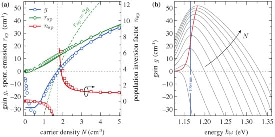
Figure 3. (a) Modal gain (blue) and rate of spontaneous emission (green), left axis, and population inversion factor (red), right axis, versus carrier density obtained from a microscopic simulation (symbols) and the analytic models (122), (123) and $n_{\mathrm{sp}}=r_{\mathrm{sp}}/g$ (solid lines) for a fixed wavelength ${\lambda }_0=1064\mathrm{nm}$. The dashed green line is the spontaneous emission computed using a constant population inversion factor $n_{\mathrm{sp}}=2$. See the Appendix A for the consideration of the gain at a fixed wavelength within the framework of the present model. (b) Microscopically computed gain spectra for carrier densities ranging from $N=1·{10}^{18}{\mathrm{cm}}^{-3}$ to $1·{10}^{19}{\mathrm{cm}}^{-3}$. The position of the fixed wavelength ${\lambda }_0$ is shown by a blue line, the peak gain position is indicated by a red line.

The gain at a fixed wavelength is modeled as

$$g=g^{\prime }{N}_{\mathrm{tr}}\ln \left[\frac{\max (N,N_{\mathrm{cl}})}{N_{\mathrm{tr}}}\right]$$

(122)

and the modal spontaneous emission as

$$r_{\mathrm{sp}}=\frac{g^{\prime }{N}_{\mathrm{tr}}}{2}\ln \left[1+{\left(\frac{N}{N_{\mathrm{tr}}}\right)}^2\right]$$

(123)

with differential gain $g^{\prime }=19·{10}^{-22}{\mathrm{m}}^2$, transparency density $N_{\mathrm{tr}}=1.7·{10}^{24}{\mathrm{m}}^{-3}$ and gain clamping density $N_{\mathrm{cl}}=7·{10}^{23}{\mathrm{m}}^{-3}$. Equation (123) exhibits the correct asymptotic behavior $r_{\mathrm{sp}}\propto N^2$ for $N\ll N_{\mathrm{tr}}$ and $r_{\mathrm{sp}}=g$ for $N\to \infty$. The agreement of $r_{\mathrm{sp}}$ between simulation and model is remarkably good without the need of introducing any new parameters. The singularity of the inversion factor at $N=N_{\mathrm{tr}}$ is clearly visible in Figure 3. If a constant value of $n_{\mathrm{sp}}=2$ is used, the spontaneous emission is considerably under- or over-estimated (depending on the respective carrier density).

10. Numerical Results for a DBR Laser

In the simulations described below we study a simple two-section DBR laser as sketched in Figure 1 and Figure 2. It consists of a 1 mm long active gain section (without Bragg grating) and a 3 mm long passive Bragg reflector section (without active layer) with a coupling coefficient of $\kappa =2{\mathrm{cm}}^{-1}$. The full set of parameters characterizing the simulated DBR laser is listed in Table 1. The usage of such DBR lasers having long reflector sections with low coupling coefficients was suggested in Ref. [16] for the first time. In fact, in Ref. [57] an intrinsic linewidth of 2 kHz at an output power of 180 mW was reported. This device had a 3 mm long gain section and a 1 mm long reflector section, where the active layer extended over the whole cavity (i.e., including the reflector section). The device studied here resembles the one presented in Ref. [60], where an intrinsic linewidth of 4 kHz at an output power of 73 mW was reported. Experimentally, the intrinsic linewidth is determined from the plateau of the frequency noise spectrum, as in the theory [61].

Table 1. Parameters of the simulated DBR laser.

Parameter	Symbol	Unit	Value	First Used
reference wavelength	${\lambda }_0$	m	$1.064·{10}^{-6}$
front facet reflectivity	$|r_0{|}^2$		$0.3$	(4)
rear facet reflectivity	$|r_L{|}^2$		0	(4)
internal optical loss (both sections)	$\alpha$	m−1	60	(3c)
group index (both sections)	$n_{\mathrm{g}}$		3.9	(2)
built-in index detuning (both sections)	$\Delta n_0$		0	(126)
Active section
length	l	m	$1·{10}^{-3}$
differential gain	$g^{\prime }$	m2	$18.62·{10}^{-22}$	(122)
$\alpha$-factor	${\tilde{\alpha }}_{\mathrm{H}}$		1	(79)
transparency carrier density	$N_{\mathrm{tr}}$	m−3	$1.7·{10}^{24}$	(122)
self-heating induced index tuning	${\nu }_s$	A−1	$9.16·{10}^{-3}$	(126)
gain clamping density	$N_{\mathrm{cl}}$	m−3	$0.8·{10}^{24}$	(122)
index clamping density	$N_{\mathrm{cl}},\mathrm{i}$	m−3	$0.01·{10}^{24}$	(125)
gain saturation power	$P_{\mathrm{sat}}$	W	$5.866$	(124)
dispersion peak amplitude	$g_{\mathcal{D}}$	m−1	50	(A3)
dispersion peak frequency detuning	${\omega }_{\mathcal{D}}$	rad s−1	0	(A3)
dispersion HWHM	${\gamma }_{\mathcal{D}}$	rad s−1	$83.25·{10}^{12}$	(A3)
thickness of active region	d	m	$4·{10}^{-6}$	(5)
width of active region	W	m	$10·{10}^{-9}$	(6)
series resistance	$R_s$	$\mathsf{\Omega }$	1	(7)
Fermi voltage derivative	$\frac{d{U}_{\mathrm{F}}}{dN}$	Vm3	$3·{10}^{-26}$	(128)
defect recombination coefficient	A	s−1	$4·{10}^8$	(127)
bimolecular recombination coefficient	B	m3 s−1	$1·{10}^{-16}$	(127)
Auger recombination coefficient	C	m6 s−1	$4·{10}^{-42}$	(127)
injection current	I	A	$[0,300]·{10}^{-3}$	(7)
Passive section
length	$L-l$	m	$3·{10}^{-3}$
coupling coefficient	$\kappa$	m−1	200	(10)
cross-heating induced index tuning	${\nu }_c$	A−1	$1.83·{10}^{-3}$	(126)

Within the active section, we assume the logarithmic gain model (122) supplemented with the nonlinear gain saturation factor

$${g(z,N,\parallel \mathsf{\Psi }\parallel }^2)=g^{\prime }(z)N_{\mathrm{tr}}(z)\ln \left[\frac{\max (N,N_{\mathrm{cl}}(z))}{N_{\mathrm{tr}}(z)}\right]\frac{1}{1+{\parallel \mathsf{\Psi }\parallel }^2/P_{\mathrm{sat}}(z)},$$

(124)

and the refractive index model with square-root-like dependency on the carrier density

$$\Delta n_N=-\frac{{\lambda }_0{\tilde{\alpha }}_{\mathrm{H}}{g}^{\prime }{N}_{\mathrm{tr}}}{2\pi }\left(\sqrt{\frac{\max (N,N_{\mathrm{cl}},\mathrm{i})}{N_{\mathrm{tr}}}}-1\right).$$

(125)

Note, that at the transparency carrier density $N_{\mathrm{tr}}$, the fixed parameter ${\tilde{\alpha }}_{\mathrm{H}}$ agrees with the $\alpha$-factor ${\alpha }_{\mathrm{H}}$ from (79), whereas $\Delta n_N$ vanishes. The $\alpha$-factor correspondingly increases for $N>N_{\mathrm{tr}}$. The value of ${\tilde{\alpha }}_{\mathrm{H}}=1$ was chosen in agreement with simulations [58] and is in basic agreement with measurements, where $\alpha$-factors between 1 and 2 for a highly-strained InGaAs quantum well were obtained, depending on the detuning [62].

Other changes of the refractive index, including self-heating-induced self- and cross-heating contributions, are modeled by [30]

$$\Delta n(z)=\Delta n_0(z)+\Delta n_T(z),\Delta n_T(z)=\left\{\begin{array}{cc}{\nu }_{s}I,\hfill & z\in [0,l]\hfill \\ {\nu }_{c}I,\hfill & z\in [l,L]\hfill \end{array}\right.,$$

(126)

where I is the injection current into the active (gain) section. We employ the commonly used cubic model for the rate of non-radiative and spontaneous recombination of the carriers in the active section

$$R(N)=AN+B{N}^2+C{N}^3,$$

(127)

is approximated by describing Shockley–Read–Hall recombination, direct band-to-band recombination and Auger recombination. Finally, the current density (7) in the gain section is approximated by

$$j(z,N)=\frac{I}{Wl}-\frac{d{U}_{\mathrm{F}}}{dN}\frac{N-\frac{1}{l}{\int }_0^{l}Ndz}{Wl{R}_s},$$

(128)

where the derivative of the Fermi voltage $d{U}_{\mathrm{F}}/dN$ is taken at a fixed carrier density.

The numerical solution of the coupled-wave Equations (2), (4), (5) and (A1) in the time domain were performed with the software package LDSL-tool developed at the Weierstrass Institute [63].

Several characteristics of the steady states obtained in the numerical simulations of the DBR laser with an upsweep of bias current are shown in Figure 4. The almost-periodic jumps towards the steady-state defined by the adjacent longitudinal optical mode and corresponding changes of the state characteristics are induced by the self-and cross-heating modeled according to (126). While the self-heating of the active section is mainly responsible for the fast shift of the lasing wavelength to longer values and periodic jumps to the shorter-wavelength state, the cross-heating induces a reduced shift of the peak wavelength of the DBR reflectivity and, therefore, the corresponding shift of the mean lasing wavelength, see Figure 4c. The maximum emitted optical power, see Figure 4a, and the minimal (averaged) carrier density, see Figure 4e, within each period coincide well with the maximum field reflection provided by the Bragg grating shown in Figure 4g.

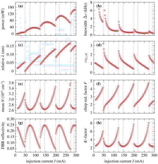
Figure 4. Simulated characteristics of the DBR laser as functions of the upsweeped injection current I. Dotted and dashed lines indicate mode jumps and maxima of the DBR reflectivity, respectively. (a) Output power $P_0$, (b) spectral linewidth $\Delta \nu$, (c) deviation from reference wavelength $\lambda -{\lambda }_0$, (d) effective $\alpha$-factor ${\alpha }_{\mathrm{eff},\mathrm{H}}$, (e) stationary carrier density $⟨N⟩$, (f) chirp reduction factor F, (g) reflection coefficient $|r^{+}{|}^2$, and (h) Petermann K-factor.

The overall decay of the estimated spectral linewidth, see Figure 4b, reflects its inverse proportionality to the field intensity, see (82). The decay of the linewidth within each period is consistent with the decrease of the modulus of the effective linewidth enhancement factor ${\alpha }_{\mathrm{H},\mathrm{eff}}$, see Figure 4d, the increase of the chirp reduction factor F shown in Figure 4f, and the behavior of Petermann’s K-factor plotted in Figure 4h. The narrowest linewidth within each period is observed at the long-wavelength flank of the DBR reflectivity just before the transition to the neighboring state. The dependence of F and ${\alpha }_{\mathrm{H}}$ on the deviation of the lasing wavelength from the peak wavelength of the DBR reflectivity confirms earlier findings [16,64,65] that F increases and ${\alpha }_{\mathrm{H},\mathrm{eff}}$ decreases at the long-wavelength flank of the reflection spectrum.

11. Outlook

The theory presented can be easily extended to take into account carrier noise. Including the source $F_N\ne 0$, we obtain instead of (73) the relation

$$\delta N={\tau }_{\mathrm{d}}{F}_N-{\tau }_{\mathrm{d}}\frac{\partial R_{\mathrm{st}}}{{\partial \left|f\right|}^2}\delta {\left|f\right|}^2.$$

(129)

Substituting this expression into (37) yields a simple modification of the Langevin force

$$F_{{\left|f\right|}^2}\to F_{{\left|f\right|}^2}+2\mathrm{Im}\frac{(\mathsf{\Phi },\frac{\partial \beta }{\partial N}{\tau }_{\mathrm{d}}{F}_N\mathsf{\Phi })}{(\mathsf{\Phi },\frac{\partial \beta }{\partial \omega }\mathsf{\Phi })}{⟨\left|f\right|}^2⟩,$$

(130)

leading to two additional additive contributions to the linewidth due to carrier noise and the cross-correlation between carrier and intensity noise. The same procedure can be applied to the calculation of the modulation of amplitude and frequency in response to an external modulation of the current injection term in (5).

In case of gain coupling, (21) has to be replaced by

$$\Delta M=\left[\begin{array}{cc}\overline{\beta }-\beta & \overline{\kappa }-\kappa \\ \overline{\kappa }-\kappa & \overline{\beta }-\beta \end{array}\right]$$

(131)

and (33) has to be supplemented by

$$\kappa =\kappa (⟨N⟩)+\frac{\partial \kappa }{\partial N}\delta N.$$

(132)

Note that for loss or gain coupling or for higher order gratings there are additional contributions to the imaginary part of $\beta$. Furthermore, the rate of stimulated recombination (6) has to be modified [66] and the diffusion coefficient (60) is varied because of non-vanishing $⟨F_{\mathrm{sp}}^{-*}(z,t)F_{\mathrm{sp}}^{+}(z^{\prime },t^{\prime })⟩\ne 0$ and its complex conjugate [22,47].

Fluctuations of the shape of the power profile can be accounted for by a linearization of (2) and (5) around a steady state, performing a Fourier transformation and solving for the fluctuations $\delta \mathsf{\Psi }$, e.g., by the Green’s function method [22] to calculate the noise spectral densities $S_{\xi }(\tilde{\omega })$ from

$$⟨{\xi }^{*}(\tilde{\omega })\xi ({\tilde{\omega }}^{\prime })⟩=2\pi S_{\xi }(\tilde{\omega })\delta (\tilde{\omega }-{\tilde{\omega }}^{\prime }),$$

(133)

where $\xi$ is the variable of interest (e.g., phase or intensity).

12. Summary

We have derived in a self-contained manner the spectral linewidth of edge-emitting multi-section semiconductor lasers starting from the time-dependent coupled-wave equations with a Langevin noise source. For this, we have expanded the forward and backward propagating fields into the longitudinal modes of the open cavity and have obtained very general expressions for the effective linewidth enhancement factor ${\alpha }_{\mathrm{H}}$ and the longitudinal excess factor of spontaneous emission (K-factor), including the effects of nonlinear gain (gain compression) and index (Kerr effect), gain dispersion, longitudinal spatial hole burning for multi-section cavity structures. We have shown that the general linewidth expression contains the effect of linewidth narrowing due to an external cavity by the chirp reduction factor F. Finally, we have investigated the dependence of the population inversion factor on the carrier density and proposed a new analytical formula. Based on the derived expressions, the spectral linewidth as well as ${\alpha }_{\mathrm{H}}$, K, and F have been calculated for a two-section DBR laser as functions of the injection current and the optical output power, taking into account the thermal detuning between gain and reflector sections. The mode jumps appearing with increasing current are accompanied by sudden rises of the spectral linewidth due to the rise of the modulus of ${\alpha }_{\mathrm{H}}$ and the drop of F.

References

- Schawlow, A.L.; Townes, C.H. Infrared and optical masers. Phys. Rev. 1958, 112, 1940. [Google Scholar] [CrossRef] [Green Version]
- Haken, H. A nonlinear theory of laser noise and coherence. I. Z. Phys. 1964, 181, 96–124. [Google Scholar] [CrossRef]
- Lax, M. Classical noise V: Noise in self-sustained oscillators. Phys. Rev. 1967, 160, 290. [Google Scholar] [CrossRef]
- Haug, H.; Haken, H. Theory of noise in semiconductor laser emission. Z. Phys. A 1967, 204, 262–275. [Google Scholar] [CrossRef]
- Scully, M.O.; Lamb, W.E., Jr. Quantum theory of an optical maser. I. General theory. Phys. Rev. 1967, 159, 208. [Google Scholar] [CrossRef]
- Risken, H. Zur Statistik des Laserlichts. Fortschr. Phys. 1968, 16, 261–308. [Google Scholar] [CrossRef]
- Petermann, K. Calculated spontaneous emission factor for double-heterostructure injection lasers with gain-induced waveguiding. IEEE J. Quantum Electron. 1979, 15, 566–570. [Google Scholar] [CrossRef]
- Siegman, A. Excess spontaneous emission in non-Hermitian optical systems. II. Laser oscillators. Phys. Rev. A 1989, 39, 1264. [Google Scholar] [CrossRef]
- Hamel, W.; Woerdman, J. Nonorthogonality of the longitudinal eigenmodes of a laser. Phys. Rev. A 1989, 40, 2785. [Google Scholar] [CrossRef]
- Wenzel, H.; Bandelow, U.; Wünsche, H.J.; Rehberg, J. Mechanisms of fast self pulsations in two-section DFB lasers. IEEE J. Quantum Electron. 1996, 32, 69–78. [Google Scholar] [CrossRef]
- Özdemir, Ş.K.; Rotter, S.; Nori, F.; Yang, L. Parity–time symmetry and exceptional points in photonics. Nat. Mater. 2019, 18, 783–798. [Google Scholar] [CrossRef]
- Henry, C.H. Theory of the linewidth of semiconductor lasers. IEEE J. Quantum Electron. 1982, 18, 259–264. [Google Scholar] [CrossRef]
- Amann, M.C. Linewidth enhancement in distributed-feedback semiconductor lasers. Electron. Lett. 1990, 26, 569–571. [Google Scholar] [CrossRef]
- Tromborg, B.; Olesen, H.; Pan, X. Theory of linewidth for multielectrode laser diodes with spatially distributed noise sources. IEEE J. Quantum Electron. 1991, 27, 178–192. [Google Scholar] [CrossRef]
- Patzak, E.; Sugimura, A.; Saito, S.; Mukai, T.; Olesen, H. Semiconductor laser linewidth in optical feedback configurations. Electron. Lett. 1983, 19, 1026–1027. [Google Scholar] [CrossRef]
- Kazarinov, R.; Henry, C.H. The relation of line narrowing and chirp reduction resulting from the coupling of a semiconductor laser to passive resonator. IEEE J. Quantum Electron. 1987, 23, 1401–1409. [Google Scholar] [CrossRef]
- Tromborg, B.; Olesen, H.; Pan, X.; Saito, S. Transmission line description of optical feedback and injection locking for Fabry–Perot and DFB lasers. IEEE J. Quantum Electron. 1987, 23, 1875–1889. [Google Scholar] [CrossRef]
- Amann, M.C.; Schimpe, R. Excess linewidth broadening in wavelength-tunable laser diodes. Electron. Lett. 1990, 26, 279–280. [Google Scholar] [CrossRef]
- Olesen, H.; Tromborg, B.; Lassen, H.; Pan, X. Mode instability and linewidth rebroadening in DFB lasers. Electron. Lett. 1992, 28, 444–446. [Google Scholar] [CrossRef]
- Schatz, R. Longitudinal spatial instability in symmetric semiconductor lasers due to spatial hole burning. IEEE J. Quantum Electron. 1992, 28, 1443–1449. [Google Scholar] [CrossRef]
- Olesen, H.; Tromborg, B.; Pan, X.; Lassen, H. Stability and dynamic properties of multi-electrode laser diodes using a Green’s function approach. IEEE J. Quantum Electron. 1993, 29, 2282–2301. [Google Scholar] [CrossRef]
- Tromborg, B.; Lassen, H.E.; Olesen, H. Traveling wave analysis of semiconductor lasers: Modulation responses, mode stability and quantum mechanical treatment of noise spectra. IEEE J. Quantum Electron. 1994, 30, 939–956. [Google Scholar] [CrossRef]
- Lax, M. Classical noise IV: Langevin methods. Rev. Mod. Phys 1966, 38, 541–566. [Google Scholar] [CrossRef]
- Lax, M. Quantum noise. IV. Quantum theory of noise sources. Phys. Rev. 1966, 145, 110. [Google Scholar] [CrossRef]
- Marani, R.; Lax, M. Spontaneous emission in non-Hermitian optical systems: Distributed-feedback semiconductor lasers. Phys. Rev. A 1995, 52, 2376. [Google Scholar] [CrossRef] [PubMed]
- Henry, C.H.; Kazarinov, R.F. Quantum noise in photonics. Rev. Mod. Phys. 1996, 68, 801. [Google Scholar] [CrossRef]
- Henry, C.H. Theory of spontaneous emission noise in open resonators and its application to lasers and optical amplifiers. J. Light. Technol. 1986, 4, 288–297. [Google Scholar] [CrossRef]
- Lasher, G.; Stern, F. Spontaneous and stimulated recombination radiation in semiconductors. Phys. Rev. 1964, 133, A553. [Google Scholar] [CrossRef]
- Agrawal, G.P.; Dutta, N.K. Semiconductor Lasers, 2nd ed.; Kluwer Academic Publishers: Boston, MA, USA, 1993. [Google Scholar] [CrossRef]
- Radziunas, M. Traveling wave modeling of nonlinear dynamics in multisection laser diodes. In Handbook of Optoelectronic Device Modeling & Simulation Volume II: Lasers, Modulators, Photodetectors, Solar Cells, and Numerical Methods; CRC Press: Boca Raton, FL, USA, 2017; pp. 153–182. [Google Scholar] [CrossRef]
- Sieber, J.; Bandelow, U.; Wenzel, H.; Wolfrum, M.; Wünsche, H.J. Travelling wave equations for semiconductor lasers with gain dispersion. WIAS Preprint 1998, 459, 1–13. [Google Scholar] [CrossRef]
- Joyce, W.B. Current-crowded carrier confinement in double-heterostructure lasers. J. Appl. Phys. 1980, 51, 2394–2401. [Google Scholar] [CrossRef]
- Zeghuzi, A.; Radziunas, M.; Wenzel, H.; Wünsche, H.J.; Bandelow, U.; Knigge, A. Modeling of current spreading in high-power broad-area lasers and its impact on the lateral far field divergence. Proc. SPIE 2018, 10526, 105261H. [Google Scholar] [CrossRef]
- Bandelow, U.; Wenzel, H.; Wünsche, H.J. Influence of inhomogeneous injection on sidemode suppression in strongly coupled DFB semiconductor lasers. Electron. Lett. 1992, 28, 1324–1326. [Google Scholar] [CrossRef]
- Lassen, H.E.; Wenzel, H.; Tromborg, B. Influence of series resistance on modulation responses of DFB lasers. Electron. Lett. 1993, 29, 1124–1126. [Google Scholar] [CrossRef]
- Ning, C.Z.; Indik, R.; Moloney, J. Effective Bloch equations for semiconductor lasers and amplifiers. IEEE J. Quantum Electron. 1997, 33, 1543–1550. [Google Scholar] [CrossRef]
- Bandelow, U.; Radziunas, M.; Sieber, J.; Wolfrum, M. Impact of gain dispersion on the spatio-temporal dynamics of multisection lasers. IEEE J. Quantum Electron. 2001, 37, 183–188. [Google Scholar] [CrossRef]
- Krüger, U.; Petermann, K. The semiconductor laser linewidth due to the presence of side modes. IEEE J. Quantum Electron. 1988, 24, 2355–2358. [Google Scholar] [CrossRef]
- Pan, X.; Tromborg, B.; Olesen, H. Linewidth rebroadening in DFB lasers due to weak side modes. IEEE Photonic Tech. L. 1991, 3, 112–114. [Google Scholar] [CrossRef]
- Gardiner, C. Stochastic Methods: A Handbook for the Natural and Social Sciences; Springer: Berlin/Heidelberg, Germany, 2009. [Google Scholar]
- Agrawal, G.P.; Roy, R. Effect of injection-current fluctuations on the spectral linewidth of semiconductor lasers. Phys. Rev. A 1988, 37, 2495. [Google Scholar] [CrossRef]
- Di Domenico, G.; Schilt, S.; Thomann, P. Simple approach to the relation between laser frequency noise and laser line shape. Appl. Opt. 2010, 49, 4801–4807. [Google Scholar] [CrossRef]
- Woods, N.D.; Payne, M.C.; Hasnip, P.J. Computing the self-consistent field in Kohn–Sham density functional theory. J. Phys. Condens. Matter 2019, 31, 453001. [Google Scholar] [CrossRef] [Green Version]
- Landau, L.D.; Lifshitz, E.M. Course of Theoretical Physics Vol. 5: Statistical Physics (Part 1); Butterworth–Heinemann: Amsterdam, The Netherlands, 1980. [Google Scholar] [CrossRef]
- Vahala, K.; Yariv, A. Semiclassical theory of noise in semiconductor lasers-Part II. IEEE J. Quantum Electron. 1983, 19, 1102–1109. [Google Scholar] [CrossRef]
- Henry, C.H. Phase noise in semiconductor lasers. J. Light. Technol. 1986, 4, 298–311. [Google Scholar] [CrossRef]
- Baets, R.G.; David, K.; Morthier, G. On the distinctive features of gain coupled DFB lasers and DFB lasers with second-order grating. IEEE J. Quantum Electron. 1993, 29, 1792–1798. [Google Scholar] [CrossRef]
- Chow, W.W.; Koch, S.W.; Sargent, M.I. Semiconductor-Laser Physics; Springer Science & Business Media: Berlin/Heidelberg, Germany, 1994. [Google Scholar] [CrossRef]
- Osinski, M.; Buus, J. Linewidth broadening factor in semiconductor lasers—An overview. IEEE J. Quantum Electron. 1987, 23, 9–29. [Google Scholar] [CrossRef]
- Champagne, Y.; McCarthy, N. Global excess spontaneous emission factor of semiconductor lasers with axially varying characteristics. IEEE J. Quantum Electron. 1992, 28, 128–135. [Google Scholar] [CrossRef]
- Wenzel, H.; Wünsche, H.J. An equation for the amplitudes of the modes in semiconductor lasers. IEEE J. Quantum Electron. 1994, 30, 2073–2080. [Google Scholar] [CrossRef]
- Pick, A.; Cerjan, A.; Liu, D.; Rodriguez, A.W.; Stone, A.D.; Chong, Y.D.; Johnson, S.G. Ab initio multimode linewidth theory for arbitrary inhomogeneous laser cavities. Phys. Rev. A 2015, 91, 063806. [Google Scholar] [CrossRef] [Green Version]
- Komljenovic, T.; Srinivasan, S.; Norberg, E.; Davenport, M.; Fish, G.; Bowers, J.E. Widely tunable narrow-linewidth monolithically integrated external-cavity semiconductor lasers. IEEE J. Sel. Top. Quantum Electron. 2015, 21, 214–222. [Google Scholar] [CrossRef]
- Tran, M.A.; Huang, D.; Bowers, J.E. Tutorial on narrow linewidth tunable semiconductor lasers using Si/III-V heterogeneous integration. APL Photonics 2019, 4, 111101. [Google Scholar] [CrossRef] [Green Version]
- Boller, K.J.; van Rees, A.; Fan, Y.; Mak, J.; Lammerink, R.E.; Franken, C.A.; van der Slot, P.J.; Marpaung, D.A.; Fallnich, C.; Epping, J.P.; et al. Hybrid integrated semiconductor lasers with silicon nitride feedback circuits. Photonics 2020, 7, 4. [Google Scholar] [CrossRef] [Green Version]
- Coldren, L.A.; Corzine, S.W.; Mashanovitch, M.L. Diode Lasers and Photonic Integrated Circuits; John Wiley & Sons: Hoboken, NJ, USA, 2012. [Google Scholar] [CrossRef]
- Spießberger, S.; Schiemangk, M.; Wicht, A.; Wenzel, H.; Erbert, G.; Tränkle, G. DBR laser diodes emitting near 1064 nm with a narrow intrinsic linewidth of 2 kHz. Appl. Phys. B 2011, 104, 813. [Google Scholar] [CrossRef]
- Wenzel, H.; Erbert, G.; Enders, P.M. Improved theory of the refractive-index change in quantum-well lasers. IEEE J. Sel. Top. Quantum Electron. 1999, 5, 637–642. [Google Scholar] [CrossRef]
- Wenzel, H.; Klehr, A.; Erbert, G.; Sebastian, J.; Tränkle, G.; Pereira, M., Jr. Effect of band gap renormalization on threshold current and efficiency of a distributed Bragg reflector laser. Appl. Phys. Lett. 2000, 76, 2653–2655. [Google Scholar] [CrossRef]
- Brox, O.; Wenzel, H.; Fricke, J.; Della Casa, P.; Maaßdorf, A.; Matalla, M.; Wenzel, S.; Wicht, A.; Knigge, A. Novel 1064 nm DBR lasers combining active layer removal and surface gratings. Electron. Lett. 2021. [Google Scholar] [CrossRef]
- Schiemangk, M.; Spießberger, S.; Wicht, A.; Erbert, G.; Tränkle, G.; Peters, A. Accurate frequency noise measurement of free-running lasers. Appl. Opt. 2014, 53, 7138–7143. [Google Scholar] [CrossRef]
- Batrak, D.V.; Sof’ya, A.B.; Borodaenko, A.V.; Drakin, A.E.; Bogatov, A.P. Simulation of the material gain in quantum-well InGaAs layers used in 1.06-μm heterolasers. Quantum Electron. 2005, 35, 316. [Google Scholar] [CrossRef]
- Radziunas, M. Longitudinal Dynamics in multisection Semiconductor Lasers. Available online: https://www.wias-berlin.de/software/ldsl/ (accessed on 22 March 2021).
- Patzak, E.; Meissner, P.; Yevick, D. An analysis of the linewidth and spectral behavior of DBR lasers. IEEE J. Quantum Electron. 1985, 21, 1318–1325. [Google Scholar] [CrossRef]
- Chaciński, M.; Schatz, R. Impact of losses in the Bragg section on the dynamics of detuned loaded DBR lasers. IEEE J. Quantum Electron. 2010, 46, 1360–1367. [Google Scholar] [CrossRef]
- Jonsson, B.; Lowery, A.J.; Olesen, H.; Tromborg, B. Instabilities and nonlinear L-I characteristics in complex-coupled DFB lasers with antiphase gain and index gratings. IEEE J. Quantum Electron. 1996, 32, 839–850. [Google Scholar] [CrossRef]
- Tronciu, V.; Wenzel, H.; Wünsche, H.J. Instabilities and Bifurcations of a DFB Laser Frequency-Stabilized by a High-Finesse Resonator. IEEE J. Quantum Electron. 2017, 53, 1–9. [Google Scholar] [CrossRef]
Publisher’s Note: MDPI stays neutral with regard to jurisdictional claims in published maps and institutional affiliations. |
© 2021 by the authors. Licensee MDPI, Basel, Switzerland. This article is an open access article distributed under the terms and conditions of the Creative Commons Attribution (CC BY) license (https://creativecommons.org/licenses/by/4.0/).