Dynamic Stability of Orthotropic Viscoelastic Rectangular Plate of an Arbitrarily Varying Thickness

Featured Application

The results obtained apply to dynamic analyses of thin-walled plates and shells of variable thickness.

Abstract

The research object of this work is an orthotropic viscoelastic plate with an arbitrarily varying thickness. The plate was subjected to dynamic periodic load. Within the Kirchhoff–Love hypothesis framework, a mathematical model was built in a geometrically nonlinear formulation, taking into account the tangential forces of inertia. The Bubnov–Galerkin method, based on a polynomial approximation of the deflection and displacement, was used. The problem was reduced to solving systems of nonlinear integrodifferential equations. The solution of the system was obtained for an arbitrarily varying thickness of the plate. With a weakly singular Koltunov–Rzhanitsyn kernel with variable coefficients, the resulting system was solved by a numerical method based on quadrature formulas. The computational algorithm was developed and implemented in the Delphi algorithmic language. The plate’s dynamic stability was investigated depending on the plate’s geometric parameters and viscoelastic and inhomogeneous material properties. It was found that the results of the viscoelastic problem obtained using the exponential relaxation kernel almost coincide with the results of the elastic problem. Using the Koltunov–Rzhanitsyn kernel, the differences between elastic and viscoelastic problems are significant and amount to more than 40%. The proposed method can be used for various viscoelastic thin-walled structures such as plates, panels, and shells of variable thickness.

1. Introduction

Thin-walled plates and shells of variable thickness are widely used in various technology fields due to the requirements for strength, durability, and thin-walled structural elements’ exterior appearance. The study of plates and shells of variable thickness made from homogeneous and inhomogeneous materials is a challenging task, and sometimes it encounters insurmountable difficulties. The difficulties are due to the solution of rather cumbersome equations, which are obtained by the desire to reflect, in mathematical modeling, the real mechanical behavior of the thin-walled structure. Variable thickness plate problems involve computational complexity, i.e., the lack of suitable universal numerical methods for solving the obtained equations, and as a consequence, unified computational algorithms.

Studies of parametric vibrations of thin-walled structures have become a separate research area in the mechanics of deformable solids. Thin-walled structures have versatile applications for various mechanical systems, in particular for plates and shells. The solution of dynamic stability problems includes the derivation of the equation of motion, discretization, and determination of areas of dynamic instability of structures.

Several publications [1,2,3] were devoted to studying the behavior of plates and shells of constant thickness under dynamic loads in an elastic formulation, where detailed reviews of these studies can be found. The research of the dynamic stability of elastic systems was started in 1964 [1]. Bolotin’s first-order approximation followed by an eigenvalue analysis gave the dynamic behavior including natural frequencies and instability load-frequency margins. The stability of the plane form of the equilibrium position of plates has been studied thoroughly in [2] for the case of compression, typically, in a uniaxial stress field, where it was assumed that the shape of buckling of the plate does not depend on buckling position’s coordinate. The article [3] is devoted to reviewing studies carried out from 1987 to 2005 in dynamic stability and parametric vibrations of plate and shell structures.

A new approach [4] based on the Amabili–Reddy higher-order shear deformation theory was implemented to modelling the geometrically nonlinear forced vibrations of laminated circular cylindrical shells. The numerical solution of discretized motion equations showed the one-to-one internal resonance for a complete circular cylindrical shell, giving rise to pitchfork bifurcations of the nonlinear response with quasiperiodic vibrations.

Theoretical and experimental aspects of nonlinear vibration and stability of shells and plates when the vibration amplitude is larger than the thickness are explained in [5]. A very good agreement between experiments and theoretical predictions was obtained for rectangular plates and circular cylindrical panels in the cases considered.

The article [6] provides an overview of publications devoted to studying nonlinear free and forced vibrations of shells made of traditional and modern materials published from 2003 to 2013. In particular, the results of studies of parametric oscillations were considered.

Nonlinear vibrations of viscoelastic thin rectangular plates were investigated in [7]. The plates were subjected to harmonic excitation. The plates’ material was modeled as a Kelvin–Voigt viscoelastic solid by retaining all the nonlinear terms. It was shown that the nonlinear response of viscoelastic plates is different from the response of the same plate with viscous damping.

Experiments presented in [8] have shown that the most significant nonlinear effect of geometrically nonlinear vibrations of rectangular plates is the increase in damping with the vibration’s amplitude. At the same time, soft materials present an increase in their stiffness with the vibration frequency. These two phenomena appearing together were explained in the framework of viscoelasticity. The nonlinear damping model for a continuous system was presented in [8]. The plate’s material was assumed to be linearly viscoelastic and modeled by the classical standard linear solid. Then, the equations of motion describing the rectangular plates’ nonlinear vibrations were derived by Lagrange equations. Rectangular plates of constant thickness with nonlinear fractional damping were investigated in [9]. It was underlined that damping increases with the vibration amplitude during nonlinear vibrations and, at the same time, soft materials such as silicone rubber increase their stiffness with the vibration frequency. The fractional linear solid model applies to describe the viscoelastic material behavior. The comparison of numerical and experimental results showed a good match.

The experimental part of the research in [10] was similar to [9]. A square silicone plate of constant thickness made of silicone with fixed edges was experimentally tested. The plate was excited with harmonic force with a frequency lower than the fundamental natural frequency. Linear and nonlinear plate responses were measured by automatic scanning laser Doppler vibrometer. The increase in damping was around 60% when the vibration amplitude was 1.6 times the plate thickness.

Out-of-plane thin membrane actuators have a vital role in micro-electromechanical systems. In [11], the nonlinear vibration control and optimal locations of actuators for a pre-tensioned membrane structure were investigated based on the nonlinear theory of plates. The theoretical and approximate solutions of nonlinear frequencies of the membrane were obtained for a complex parametric study of the behavior of membranes, and the discrepancies between the two solutions under different vibration amplitudes were discussed.

The dynamic instability of thin laminated composite rectangular plates with various length–width and length–thickness aspect ratios subjected to harmonic in-plane loading has been theoretically studied [12]. The equations of motion of the plate were developed using the von Kármán type of plate equation considering geometric nonlinearity. The equations were solved by using Galerkin’s technique. Dynamically unstable regions and both stable- and unstable-solution amplitudes of the steady-state vibrations were obtained by applying Bolotin’s method.

Dynamic instability and nonlinear parametric vibrations of multilayer composite plates subjected to the action of periodic compressive loads in the plane applied along two opposite edges were considered in [13]. A system of ordinary differential nonlinear equations of the second-order Mathieu–Hill with periodic coefficients was obtained for determining the regions of dynamic instability and nonlinear parametric oscillations based on the Bolotin method. The influence of various parameters on the dynamic stability and nonlinear parametric oscillations was investigated: static load, dynamic load, elongation, boundary conditions, orthotropy, and damping coefficient.

Functionally graded materials, the material properties of which are varied along the thickness direction, are widely used in aerospace structures, nuclear reactors, and other structures with high functional performance [14]. The nonlinear dynamic instability of a functionally graded rectangular plate of constant thickness was investigated [15]. The plate was made by mixing two different materials, metal on one surface and ceramic on the other surface. The plate was subjected to nonuniform loading. The equations of motion used higher-order shear deformation theory considering von Kármán geometric nonlinearity. Galerkin’s method was used to reduce the nonlinear governing partial differential equations into ordinary differential equations describing the plate’s nonlinear dynamic instability. Bolotin’s method was used to obtain the boundaries of dynamic instability regions. Effects of power index, span-to-thickness ratio, aspect ratio, static load factor, boundary conditions, and various types of linearly varying loadings and parabolically distributed loadings were studied.

Analytical studies on the dynamic instability analysis of a functionally graded constant thickness skew plate (in the form of the parallelogram) made by mixing ceramic and metal materials were presented in [16]. The plate was subjected to uniform and linearly varying in-plane periodic loadings with four different types of boundary conditions. The total energy functional of the plate was formulated based on Reddy’s third-order shear deformation theory. The energy functional was converted into a set of ordinary differential equations (Mathieu–Hill equations) using the Rayleigh–Ritz method in conjunction with BCOPs. The solution of the Mathieu–Hill equations described the dynamic instability behavior of the skew plate. The instability regions were traced using the Bolotin method.

The parametric instability of a functionally graded polymer-based graphene-reinforced nanocomposite plate of constant thickness was investigated in [17]. The plate comprised multiple graphene platelet reinforced composite layers in which graphene platelets are uniformly distributed in each layer with graphene platelet concentration varying layerwise across the plate thickness. The plate was subjected to periodic uniaxial in-plane force and a uniform temperature rise. The basic equations were derived from the theory of first-order shear deformation. The problems were solved using the differential quadrature approach in combination with the Bolotin method.

The instability of rectangular plates due to parametric resonance was considered in [18]. The partial differential equation was derived using the extended Hamilton principle. Using the Galerkin method, the resulting equation was reduced to a system of ordinary differential equations. Semianalytical results were obtained for various plate boundary conditions, confirmed by numerical simulations and other published results.

The boundaries of instability of axially accelerating plates with internal resonance were studied in [19]. A connection was introduced between acceleration and tensions changing in the longitudinal direction. The main equation and the corresponding boundary conditions were derived from the generalized Hamilton’s principle. The effects of internal resonances and inhomogeneous boundary conditions at the boundaries of instability were distinguished. Multiple scales established modified conditions of solvability in the main parametric and internal resonances. The Routh–Hurwitz criterion was introduced to determine the boundaries of instability. The influence of the coefficient of viscoelasticity and the coefficient of viscous damping on instability boundaries was investigated. Abnormal instability boundaries were detected upon the application of the internal resonance. The phenomenon of local zigzag and V-shaped boundaries was explained in terms of modal interactions. Numerical calculations of differential quadrature circuits for the first four complex frequencies, the first four complex modes, and stability boundaries were used to confirm the analytical method’s results.

The R-functions theory was used for solving dynamic problems of the theory of plates and shells, connected with the construction of the basic function in the case of an arbitrary domain [20,21,22,23,24,25,26]. In [20], dynamic instability and nonlinear parametric vibrations of multilayer plates of complex shapes were investigated. A numerical–analytical method based on a combination of the theory of R-functions and the variational method was proposed. Instability regions and response curves were plotted for various types of materials and load parameters.

In [21], using the theory of R-functions, a method was proposed for studying dynamical instability and nonlinear parametric vibrations of laminated plates. The plates had complex shapes and different cutouts. The structure of the plate was symmetrical concerning its middle surface, consisting of layers of constant thickness. The loads consisted of a periodic in-plane load and static load. The mathematical setting was carried out within the framework of the classical theory based on the Kirchhoff–Love hypothesis. The proposed method was based on the first-order shear deformation theory and the classical plate theory. A plane stress analysis was carried out using the variational Ritz method and the R-functions theory. The obtained results were applied to investigate buckling and parametric vibrations of laminated plates.

In [22], the problem of nonlinear vibrations and analysis of the stability of multilayer symmetric plates of complex shape, loaded with a static or periodic load in the plane, was considered. An approach based on the application of the theory of R-functions and variational methods was proposed. The proposed approach was demonstrated in testing tasks and applied to laminated plates with cutouts. The influence of geometrical parameters, load, boundary conditions on stability regions, and nonlinear oscillations was investigated.

The paper [23] proposes a method for studying parametric vibrations of orthotropic plates of complex shape for various types of boundary conditions, based on variational methods in combination with the theory of R-functions. Specific tasks were solved. Regions of dynamic instability and deflection depending on the frequency and excitation time were plotted for a plate of complex shape.

R-functions theory was used to study the free vibrations and dynamic instability of a symmetrically layered plate [24]. The plate was subjected to combined static and periodic axial forces. The problem was considered within the framework of the classical theory of plates. The solution of problems was based on the variational Ritz method’s joint application, the Galerkin procedure, the theory of R-functions, and Bolotin’s theory. The influence of the plate’s geometric parameters and the mechanical characteristics of the material on the parametric resonance was studied.

The combination of the R-function theory and variational methods was proposed in [25,26,27]. The parametric vibrations of T-shape, rectangular, and rectangular cutout orthotropic plates of constant thickness were investigated for various boundary conditions [25,27]. Using the Kirchhoff–Love hypothesis, the motion equations were built. The proposed hybrid approach is based on the combination of the R-functions method and the variation Ritz method. The numerical analysis showed that one mode of approximation cannot be used in all nonlinear dynamics of the orthotropic plates, particularly during their chaotic dynamics.

A numerical–analytical method was proposed in [26] for studying parametric vibrations of plates under the action of periodic loads applied in the middle plane. Equations of motion were obtained within the framework of classical theory. The developed approach based on applying the theory of R-functions and variational methods was used to solve the equations, making it possible to study plates of arbitrary geometric shapes with various boundary conditions. The authors used the Bolotin method to construct the region of dynamic instability. The results obtained using the developed approach were compared with the results of other authors.

In [28], the problem of dynamic stability of laminated composite plates under a combination of biaxial periodic loads and bending was considered based on the theory of plates, taking into account shear deformation. A system of second-order ordinary differential equations with periodic coefficients of the Mathieu–Hill type was obtained. The Bolotin method was applied to determine the areas of dynamic instability. The influence of modules’ ratio, the number of layers, and static and dynamic parameters of the load on the dynamic instability was investigated.

The article [29] considered the dynamic stability of a viscoelastic plate under a periodic load. A differential equation was obtained that describes the dynamic stability of the plate. The solution was sought by the method of separation of variables. Linear differential equations of the third order were obtained for the time function. The prime instability domain position was affected by relaxation time and the correlation between long-term and instantaneous moduli of elasticity.

In [30], using the Bubnov–Galerkin method, the equations of motion of a shallow shell in a mixed form under the action of a longitudinal harmonic load were reduced to a discrete system with finite degrees of freedom. The chaotic behavior of systems with different degrees of freedom was analyzed. It was shown that by increasing the parameter of periodical longitudinal exciting, the investigated system starts to lose the regular behavior, forgetting its initial state, and chaotic dynamics occur.

The parametric instability of rectangular plates made of functionally graded material, subjected to biaxial periodic loading in the plane, was investigated [31]. The equations of motion were constructed, taking into account shear deformation. Hamilton’s Principle was used to transform the basic equations into a linear system of Mathieu–Hill equations. With the help of the Floquet theory, areas of dynamic instability were determined. The influence of various parameters on areas of dynamic instability was investigated.

Viscoelastic rectangular plates with constant thickness, shells, and cylindrical panels were studied in a geometrically nonlinear formulation [32,33,34,35]. The models were based on the Kirchhoff–Love hypothesis. The problem was reduced to a system of nonlinear ordinary integrodifferential equations by using the Bubnov–Galerkin method. The resulting system with a weakly singular Koltunov–Rzhanitsyn kernel was solved using a numerical method based on quadrature formulas.

The article [36] was devoted to studying the stability of parametric vibrations of an isolated symmetric cross-ply laminated plate system. The plate system’s mechanical model was given as an isolated symmetric cross-ply laminated constant thickness rectangular plate subjected to uniformly distributed stochastic in-plane time-dependent loading. The influence of transverse shear on the laminated plate was taken into account. The equations of motion were derived based on the shear deformation theory and the Kirchhoff–Love theory [37].

As models of viscoelastic material, the Maxwell and Kelvin–Voigt constitutive equations and the standard solid model are the simplest and most used by many researchers. These models are reduced to solving differential equations with initial conditions. The use of differential dependencies between stress and strain in dynamic problems of viscoelasticity theory leads to a specific inaccuracy. The inaccuracy is especially noticeable at the initial moment. The reason for this inaccuracy is that the strain rate and stress rate according to these models will always be finite.

In contrast, the experiment shows an arbitrarily high rate of deformation. It should be noted that the inaccuracy made at the initial moment significantly affects the final result of the study, i.e., there is an accumulation of errors. There will be no accumulation of errors if the integral relationship between stresses and strains uses a weakly singular Koltunov–Rzhanitsyn kernel with weakly singular features of the Abel type [38,39,40,41]. The use of integral dependence significantly expands the class of problems to be solved in the theory of viscoelasticity. Simultaneously, mathematical models with integral dependence are reduced to solving complex systems of nonlinear integrodifferential equations by numerical methods [42].

The available literature analysis showed a small number of publications on nonlinear vibrations and dynamic stability of thin viscoelastic plates and shells of variable thickness. Reviewed studies show that the calculation of plates and shells of variable thickness faces significant computational difficulties. The calculation of plates and shells of this kind requires the solution of rather cumbersome equations [43,44,45]. There is a lack of suitable universal numerical methods and unified computational algorithms for solving the obtained equations.

It is necessary to carry out research in a geometrically nonlinear formulation and consider the material’s viscoelastic properties to obtain a performance of the stress–strain state of thin-walled structural elements of variable thickness.

The research object is an orthotropic viscoelastic plate with an arbitrarily varying thickness subjected to a periodic compressive force in the plate’s plane. The research subjects were the plate’s deformations, the vibration modes of the plate, the vibration amplitudes, and the change in vibration over time depending on the thickness (geometry) of the plate, the ratio of the frequencies of the periodic force, the natural frequencies of the plate, and the viscoelastic properties of the plate material.

This research aimed to develop the theory of the orthotropic plate’s dynamic stability, considering the plate’s materials’ viscoelastic properties.

The research objectives are as follows:

-

Development of a mathematical model of the dynamic behavior of plates of variable thickness;

-

Development of a method for numerical solutions of nondecaying systems of nonlinear integrodifferential equations with weakly singular kernels of an orthotropic viscoelastic plate of variable thickness under the influence of external periodic loads;

-

Clarification of the orthotropic viscoelastic plate’s dynamic stability with varied mechanical and geometric parameters of the plate.

2. Methods

An analytical–numerical method was used to study the nonlinear vibrations of an orthotropic rectangular plate of variable thickness under the action of a uniformly distributed vibration load leading (at certain combinations of natural vibration frequencies and disturbing forces) to parametric resonance.

2.1. Analytical and Numerical Method

Consider an anisotropic viscoelastic rectangular plate of an arbitrarily varying thickness $h\left(x,y\right)$ with sides $a$ and $b$ under the action of axial dynamic loads along the side $a$ (Figure 1). In the general case, the law of change in thickness $h$ can be specified analytically as the function of the $x$ and $y$ coordinates. This function $h\left(x,y\right)$ must have continuous second derivatives in each of the $x$ and $y$ coordinates. Further, a certain form of dependence (106) is used in numerical examples, but it is not the only possible one.

The mathematical model of the problem in a geometrically nonlinear formulation follows the classical Kirchhoff–Love theory. The system of equations of motion within the framework of the chosen theory has the following form [46,47]:

$$\frac{\partial N_x}{\partial x}+\frac{\partial N_{xy}}{\partial y}+p_x-\rho h\frac{{\partial }^{2}u}{\partial t^2}=0$$

(1)

$$\frac{\partial N_{xy}}{\partial x}+\frac{\partial N_y}{\partial y}+p_y-\rho h\frac{{\partial }^{2}v}{\partial t^2}=0$$

(2)

$$\begin{gathered} \frac{{\partial }^2{M}_x}{\partial x^2}+\frac{{\partial }^2{M}_y}{\partial y^2}+2\frac{{\partial }^{2}H}{\partial x\partial y}+\frac{\partial }{\partial x}\left(N_x\frac{\partial w}{\partial x}+N_{xy}\frac{\partial w}{\partial y}\right)+ \\ +\frac{\partial }{\partial y}\left(N_{xy}\frac{\partial w}{\partial x}+N_y\frac{\partial w}{\partial y}\right)+P_x\left(t\right)\frac{{\partial }^{2}w}{\partial x^2}+q-\rho h\frac{{\partial }^{2}w}{\partial t^2}=0. \end{gathered}$$

(3)

Here, $N_x$ and $N_y$ are the normal forces per unit length; $N_{xy}$ is the shear force; $M_x$ and $M_y$ are the bending moments, $H$ is the torque moment; $p_x$ and $p_y$ are the in-plane loads per unit area; $q$ is the normal distributed load per unit area; $P_x\left(t\right)$ is the compressive force per unit length applied to the plate edge; $\rho$ is the density of the material; and $u$, $v$, and $w$ are the components of the displacement vector $\left\{U\right\}$ in the directions of the axes $Ox$, $Oy$, and $Oz$, respectively. The compressive force $P_x\left(t\right)$ is applied to the side of dimension $b$ and is a function of time according to the law $P_x=P_0+P_t\cos \left(\theta t\right)$, where $P_0$ is the constant part of the load, $P_t$ is the amplitude of the variable part, and $\theta$ is the frequency of the load pulsations.

The system of Equations (1)–(3) is supplemented by the corresponding boundary conditions [46], which will be used to solve the problems:

1.

All edges are simply supported:

at $x=0,a$: $u=0,$ $v=0,$ $w=0$; $M_x=0$; at $y=0,b$:$u=0,$ $v=0,$ $w=0$; $M_y=0$.

2.

All edges are clamped:

at $x=0,a$: $u=0,$ $v=0,$ $w=0$; $\frac{\partial w}{\partial x}=0$; at $y=0,b$:$u=0,$ $v=0,$ $w=0$; $\frac{\partial w}{\partial y}=0$.

3.

Two opposite edges are simply supported, the other two edges are clamped:

at $x=0,a$: $u=0,$ $v=0,$ $w=0$; $\frac{\partial w}{\partial x}=0$; at $y=0,b$:$u=0,$ $v=0,$ $w=0$; $M_y=0$.

The initial conditions at $t=0$ [46] are as follows:

$u\left(x,y,0\right)=u_0\left(x,y\right)$,${\dot{u}}_0\left(x,y,0\right)={\dot{u}}_0\left(x,y\right)$, $v\left(x,y,0\right)=v_0\left(x,y\right)$, $\dot{v}\left(x,y,0\right)={\dot{v}}_0\left(x,y\right)$,

$w\left(x,y,0\right)=w_0\left(x,y\right)$, and $\dot{w}\left(x,y,0\right)={\dot{w}}_0\left(x,y\right)$.

Here, $u_0\left(x,y\right)$, $v_0\left(x,y\right)$, $w_0\left(x,y\right)$, ${\dot{u}}_0\left(x,y\right)$, ${\dot{v}}_0\left(x,y\right)$, and ${\dot{w}}_0\left(x,y\right)$ are given functions.

2.2. Computational Methods

The solution of the system (1)–(3) is obtained by using the Bubnov–Galerkin method based on a polynomial approximation of the deflection and displacements; discretization is performed in spatial variables at each moment and is reduced to solving systems of nonlinear integrodifferential equations with weakly singular kernels with variable coefficients. The improved numerical method [48] based on quadrature formulas was applied to solve the obtained nondecaying system with a weakly singular Koltunov–Rzhanitsyn kernel [40,41,49].

A relaxation kernel $\Gamma \left(\mathrm{t}\right)=A{e}^{-\beta t}{t}^{\alpha -1}, \left(0<\alpha <1\right)$ with three rheological parameters was first proposed in [40]. Publications [40,41] explain a method for determining the parameters $A$, $\alpha$, and $\beta$. In [41], these parameters are tabulated. The parameters of specific materials are determined by combining the experimental curve and the theoretical curve plotted in logarithmic coordinates.

The number of relaxation kernels for isotropic and orthotropic plates is different:

(i)

The mechanical parameters of the viscoelastic isotropic are the same in all directions. Therefore, the viscoelastic properties of the plate material are described with one core with three rheological parameters.

(ii)

Mechanical parameters of viscoelastic orthotropic plates are different in two mutually perpendicular directions, coinciding with the directions of the coordinate axes. In this case, there are five different relaxation nuclei. In addition, there are three rheological parameters in each relaxation core. Thus, there are 15 different rheological parameters in total.

After applying the Bubnov–Galerkin method, most of the dynamic problems of viscoelastic thin-walled structures are reduced to solving nondecaying systems of integrodifferential equations of the following form:

$$\begin{gathered} \begin{array}{c}{\displaystyle \sum _{n=1}^N{\displaystyle \sum _{m=1}^M(a_{klnm}{\ddot{u}}_{nm}+{\lambda }_{nmkl}^2{u}_{nm})={{\rm X}}_{nm}(t,u_{11},\dots ,u_{NM},v_{11},\dots ,}}{v}_{NM},w_{11},\dots ,w_{NM},\\ {\displaystyle \underset{0}{\overset{t}{\int }}{\varphi }_{1nm}\left(t,\tau ,u_{11}\dots ,u_{NM},v_{11},\dots ,v_{NM},w_{11},\dots ,w_{NM}\right)d\tau ),}\end{array} \\ \begin{array}{c}{\displaystyle \sum _{n=1}^N{\displaystyle \sum _{m=1}^M(b_{klnm}{\ddot{v}}_{nm}+{\chi }_{nmkl}^2{v}_{nm})={{\rm Y}}_{nm}(t,u_{11},\dots ,u_{NM},v_{11},\dots ,}}{v}_{NM},w_{11},\dots ,w_{NM},\\ {\displaystyle \underset{0}{\overset{t}{\int }}{\varphi }_{1nm}\left(t,\tau ,u_{11}\dots ,u_{NM},v_{11},\dots ,v_{NM},w_{11},\dots ,w_{NM}\right)d\tau ),}\end{array} \\ \begin{array}{c}{\displaystyle \sum _{n=1}^N{\displaystyle \sum _{m=1}^M(c_{klnm}{\ddot{w}}_{nm}+{\omega }_{nmkl}^2{w}_{nm})=Z_{nm}(t,u_{11},\dots ,u_{NM},v_{11},\dots ,}}{v}_{NM},w_{11},\dots ,w_{NM},\\ {\displaystyle \underset{0}{\overset{t}{\int }}{\psi }_{1nm}\left(t,\tau ,u_{11}\dots ,u_{NM},v_{11},\dots ,v_{NM},w_{11},\dots ,w_{NM}\right)d\tau )}\end{array} \\ {u}_{nm}\left(0\right)=u_{0nm},{\dot{u}}_{nm}\left(0\right)={\dot{u}}_{0nm},v_{nm}\left(0\right)=v_{0nm},{\dot{v}}_{nm}\left(0\right)={\dot{v}}_{0nm},w_{nm}\left(0\right)=w_{0nm},{\dot{w}}_{nm}\left(0\right)={\dot{w}}_{0nm}, \\ n=1,2,\dots ,N;m=1,2,\dots ,M, \end{gathered}$$

(4)

where $u_{nm}=u_{nm}(t),$ $v_{nm}=v_{nm}(t),$ and $w_{nm}=w_{nm}(t)$ are unknown functions of time; $X_{nm},Y_{nm},Z_{nm},{\varphi }_{1nm},{\varphi }_{1nm},{\psi }_{1nm}$ are continuous functions in the field of changing arguments; and $a_{klnm},$ $b_{klnm},$ $c_{klnm},$ ${\lambda }^2{}_{klnm},$ ${\chi }^2{}_{klnm},$ and ${\omega }^2{}_{klnm}$ are given constant numbers.

Integration of system (4) twice on $t$ leads to its integral form. Then, $t=t_i,$ $t_i=i\Delta t,$ $i=1,2,\dots$ (Δt = const is the interpolation step) is assumed. Replacing integrals with quadrature formulas for calculations $u_{nm}=u_{nm}(t_i)$, $v_{nm}=v_{nm}(t_i)$, and $w_{nm}=w_{nm}(t_i)$ results in the following system:

$$\begin{gathered} \begin{array}{c}{\displaystyle \sum _{n=1}^N{\displaystyle \sum _{m=1}^M{a}_{klnm}}}{u}_{pnm}={\displaystyle \sum _{n=1}^N{\displaystyle \sum _{m=1}^M{a}_{klnm}}}(u_{0nm}+{\stackrel{•}{u}}_{onm}{t}_p)+\\ +{\displaystyle \sum _{j=0}^{p-1}{A}_j}(t_p-t_j)\{{\mathrm{X}}_{kl}(\begin{array}{c}\\ \end{array}{t}_j,u_{j11},\dots ,u_{jNM},v_{j11},\dots ,v_{jNM},w_{j11},\dots ,w_{jNM},\end{array} \\ {\displaystyle \sum _{s=0}^j{B}_s{\varphi }_{1kl}(t_j,t_s,}{u}_{s11},\dots ,u_{sNM},v_{s11},\dots ,v_{sNM},w_{s11},\dots ,w_{sNM})\begin{array}{c}\\ \end{array})-{\lambda }_{nmkl}^2{u}_{jkl}\}, \\ \begin{array}{c}{\displaystyle \sum _{n=1}^N{\displaystyle \sum _{m=1}^M{b}_{klnm}}{v}_{pnm}}={\displaystyle \sum _{n=1}^N{\displaystyle \sum _{m=1}^M{b}_{klnm}}}(v_{0nm}+{\stackrel{•}{v}}_{onm}{t}_p)+\\ +{\displaystyle \sum _{j=0}^{p-1}{A}_j}(t_p-t_j)\{{\mathrm{Y}}_{kl}(\begin{array}{c}\\ \end{array}{t}_j,u_{j11},\dots ,u_{jNM},v_{j11},\dots ,v_{jNM},w_{j11},\dots ,w_{jNM},\end{array} \\ {\displaystyle \sum _{s=0}^j{B}_s{\varphi }_{1kl}(t_j,t_s,}{u}_{s11},\dots ,u_{sNM},v_{s11},\dots ,v_{sNM},w_{s11},\dots ,w_{sNM})\begin{array}{c}\\ \end{array})-{\chi }_{nmkl}^2{v}_{jkl}\}, \\ \begin{array}{c}{\displaystyle \sum _{n=1}^N{\displaystyle \sum _{m=1}^M{c}_{klnm}{w}_{pnm}}}={\displaystyle \sum _{n=1}^N{\displaystyle \sum _{m=1}^M{c}_{klnm}}}(w_{0nm}+{\dot{w}}_{onm}{t}_p)+\\ +{\displaystyle \sum _{j=0}^{p-1}{A}_j}(t_p-t_j)\{{\mathrm{Z}}_{kl}(\begin{array}{c}\\ \end{array}{t}_j,u_{j11},\dots ,u_{jNM},v_{j11},\dots ,v_{jNM},w_{j11},\dots ,w_{jNM},\end{array} \\ {\displaystyle \sum _{s=0}^j{B}_s{\psi }_{1kl}(t_j,t_s,}{u}_{s11},\dots ,u_{sNM},v_{s11},\dots ,v_{sNM},w_{s11},\dots ,w_{sNM})\begin{array}{c}\\ \end{array})-{\omega }_{nmkl}^{}{w}_{jkl}\} \end{gathered}$$

(5)

The next stage of the numerical method is the regularization of nonlinear integrodifferential Equation (5) with weakly singular kernels. By changing variables

$$t-\tau =z^{\frac{1}{\alpha }}, 0\le z\le t^{\alpha }(0<\alpha <1)$$

(6)

the integral at the Koltunov–Rzhanitsyn kernel with a singularity of the following form:

$$A{\displaystyle \underset{0}{\overset{t}{\int }}{(t-\tau )}^{\alpha -1}}\exp (-\beta (t-\tau ))w(\tau )d\tau$$

(7)

takes the form

$$\frac{A}{\alpha }{\displaystyle \underset{0}{\overset{t^{\alpha }}{\int }}}\exp (-\beta z^{\frac{1}{\alpha }})w(t-z^{\frac{1}{\alpha }})dz$$

(8)

After the change of variables, the integrand concerning z becomes regular. Direct replacement of the integrals in the system (5) by a sum over some quadrature formula yields a numerical solution to the numerical solution of system (5).

The trapezium formula used is

$$\frac{A}{\alpha }{\displaystyle \sum _{k=0}^i{B}_k\exp (-\beta t_k)w_{i-k}},$$

(9)

where the coefficients are

$$\begin{gathered} B_0=\frac{1}{2}{(\Delta t)}^{\alpha };B_i=\frac{1}{2}{(\Delta t)}^{\alpha }(i^{\alpha }-{(i-1)}^{\alpha }); \\ {B}_k=\frac{1}{2}{(\Delta t)}^{\alpha }({(k+1)}^{\alpha }-{(k-1)}^{\alpha }),k=\overline{1,i-1}. \end{gathered}$$

(10)

Thus, due to the double integration of the original system (4) over the time t and the use of the quadrature formula, system (5) is obtained to find deflections $w_{nm}=w_{nm}(t_i)$ and displacements $u_{nm}=u_{nm}(t_i),$ $v_{nm}=v_{nm}(t_i)$. The solutions of the system of Equation (5) are found by the Gauss method.

3. Results and Discussion

3.1. Analytical Solution for an Orthotropic Viscoelastic Rectangular Plate of Variable Thickness

This section presents the obtention of the analytical solution for the dynamic stability of an orthotropic viscoelastic rectangular plate of variable thickness. The solution is based on the integral relationship between stresses and strains using the weakly singular Koltunov–Rzhanitsyn kernel with weakly singular features of the Abel type.

The components of the vector of forces $\left\{N\right\}=\left(N_x,N_y,N_{xy}\right)$ and moments $\left\{M\right\}=\left(M_x,M_y,M_{xy}\right)$ for a plate of symmetric structure in matrix form can be written as follows:

$$\left\{N\right\}={\left\{N_x,N_y,N_{xy}\right\}}^T=\left[C\right]\cdot \left\{\epsilon \right\}$$

(11)

$$\left\{M\right\}={\left\{M_x,M_y,M_{xy}\right\}}^T=\left[D\right]\cdot \left\{\chi \right\}$$

(12)

where

$$\left\{\epsilon \right\}={\left({\epsilon }_x,{\epsilon }_y,{\epsilon }_{xy}\right)}^T$$

(13)

$$\left\{\chi \right\}={\left({\chi }_x,{\chi }_y,{\chi }_{xy}\right)}^T$$

(14)

$${\epsilon }_x=\frac{\partial u}{\partial x}+\frac{1}{2}\left[{\left(\frac{\partial w}{\partial x}\right)}^2-{\left(\frac{\partial w_0}{\partial x}\right)}^2\right]$$

(15)

$${\epsilon }_y=\frac{\partial v}{\partial y}+\frac{1}{2}\left[{\left(\frac{\partial w}{\partial y}\right)}^2-{\left(\frac{\partial w_0}{\partial y}\right)}^2\right]$$

(16)

$${\epsilon }_{xy}=\frac{\partial u}{\partial x}+\frac{\partial v}{\partial y}+\frac{\partial w}{\partial x}\frac{\partial w}{\partial y}-\frac{\partial w_0}{\partial x}\frac{\partial w_0}{\partial y}$$

(17)

$${\chi }_x=-\frac{{\partial }^{2}w}{\partial x^2}$$

(18)

$${\chi }_y=-\frac{{\partial }^{2}w}{\partial y^2}$$

(19)

$${\chi }_{xy}=-\frac{{\partial }^{2}w}{\partial x\partial y}$$

(20)

The stiffness matrixes $\left[C\right]$ and $\left[D\right]$ are given as follows [47]:

$$C=\left(\begin{array}{ccc}{C}_{11}& C_{12}& C_{16}\\ C_{12}& C_{22}& C_{26}\\ C_{16}& C_{26}& C_{66}\end{array}\right)$$

(21)

$$D=\left(\begin{array}{ccc}{D}_{11}& D_{12}& D_{16}\\ D_{12}& D_{22}& D_{26}\\ D_{16}& D_{26}& D_{66}\end{array}\right)$$

(22)

where the coefficients of the stiffness matrixes $C_{ij}$ and $D_{ij}$ (ij = 11, 22, 12, 16, 26, 66), depending on the mechanical characteristics of the viscoelastic material, and the mass per unit area coefficient $m$ are determined as follows:

$$C_{ij}={\displaystyle \underset{-\frac{h\left(x,y\right)}{2}}{\overset{\frac{h\left(x,y\right)}{2}}{\int }}{B}_{ij}\left(1-{\Gamma }_{ij}^{\ast }\right)}dz$$

(23)

$$D_{ij}={\displaystyle \underset{-\frac{h\left(x,y\right)}{2}}{\overset{\frac{h\left(x,y\right)}{2}}{\int }}{B}_{ij}\left(1-{\Gamma }_{ij}^{\ast }\right)}{z}^{2}dz, (i,j=1, 2, 6)$$

(24)

$$m={\displaystyle \underset{-\frac{h\left(x,y\right)}{2}}{\overset{\frac{h\left(x,y\right)}{2}}{\int }}\rho }dz$$

(25)

where $B_{ij}$ is the coefficient of the stiffness [47] and ${\Gamma }^{\ast },{\Gamma }_{ij}^{\ast }$ are integral operators with relaxation kernels $\Gamma \left(t\right)$ and ${\Gamma }_{ij}\left(t\right)$, respectively:

$${\Gamma }^{\ast }\varphi ={\displaystyle \underset{0}{\overset{1}{\int }}\Gamma \left(t-\tau \right)\varphi \left(\tau \right)d\tau }$$

(26)

$${\Gamma }_{ij}^{\ast }\varphi ={\displaystyle \underset{0}{\overset{1}{\int }}{\Gamma }_{ij}\left(t-\tau \right)\varphi \left(\tau \right)d\tau }, i,j=1, 2$$

(27)

In operator form, the system of equations of motion (1)–(3) is as follows:

$$L_{11}u+L_{12}v=-L_{14}w+m\frac{{\partial }^{2}u}{\partial t^2}$$

(28)

$$L_{21}u+L_{22}v=-L_{24}w+m\frac{{\partial }^{2}v}{\partial t^2}$$

(29)

$$L_{33}w=-L_{34}w+m\frac{{\partial }^{2}w}{\partial t^2}$$

(30)

Then,

$$L_{11}=C_{11}\frac{{\partial }^2}{\partial x^2}+2C_{16}\frac{{\partial }^2}{\partial x\partial y}+C_{66}\frac{{\partial }^2}{\partial y^2}$$

(31)

$$L_{12}=L_{21}=C_{16}\frac{{\partial }^2}{\partial x^2}+\left(C_{12}+C_{66}\right)\frac{{\partial }^2}{\partial x\partial y}+C_{26}\frac{{\partial }^2}{\partial y^2}$$

(32)

$$L_{22}=C_{66}\frac{{\partial }^2}{\partial x^2}+2C_{26}\frac{{\partial }^2}{\partial x\partial y}+C_{22}\frac{{\partial }^2}{\partial y^2}$$

(33)

$$L_{33}=D_{11}\frac{{\partial }^4}{\partial x^4}+2\left(D_{12}+2D_{66}\right)\frac{{\partial }^4}{\partial x^2\partial y^2}+4D_{16}\frac{{\partial }^4}{\partial x^3\partial y}+4D_{26}\frac{{\partial }^4}{\partial x\partial y^3}+D_{22}\frac{{\partial }^4}{\partial y^4}$$

(34)

$$\begin{gathered} L_{14}\left(u,v,w,C_{ij}\right)=\frac{\partial }{\partial x}\{\frac{1}{2}{C}_{11}\left[{\left(\frac{\partial w}{\partial x}\right)}^2-{\left(\frac{\partial w_0}{\partial x}\right)}^2\right]+\frac{1}{2}{C}_{12}\left[{\left(\frac{\partial w}{\partial y}\right)}^2-{\left(\frac{\partial w_0}{\partial y}\right)}^2\right]+ \\ +C_{16}\left[\frac{\partial w}{\partial x}\frac{\partial w}{\partial y}-\frac{\partial w_0}{\partial x}\frac{\partial w_0}{\partial y}\right]\}+\frac{\partial }{\partial y}\{\frac{1}{2}{C}_{16}\left[{\left(\frac{\partial w}{\partial x}\right)}^2-{\left(\frac{\partial w_0}{\partial x}\right)}^2\right]+\frac{1}{2}{C}_{26}\left[{\left(\frac{\partial w}{\partial y}\right)}^2-{\left(\frac{\partial w_0}{\partial y}\right)}^2\right]+ \\ +C_{66}\left[\frac{\partial w}{\partial x}\frac{\partial w}{\partial y}-\frac{\partial w_0}{\partial x}\frac{\partial w_0}{\partial y}\right]\}+\left[\frac{\partial u}{\partial x}+\frac{1}{2}{\left(\frac{\partial w}{\partial x}\right)}^2-\frac{1}{2}{\left(\frac{\partial w_0}{\partial x}\right)}^2\right]\left(\frac{\partial C_{11}}{\partial x}+\frac{\partial C_{16}}{\partial y}\right)+ \\ +\left[\frac{\partial v}{\partial y}+\frac{1}{2}{\left(\frac{\partial w}{\partial y}\right)}^2-\frac{1}{2}{\left(\frac{\partial w_0}{\partial y}\right)}^2\right]\left(\frac{\partial C_{12}}{\partial x}+\frac{\partial C_{26}}{\partial y}\right)+\left(\frac{\partial u}{\partial y}+\frac{\partial v}{\partial x}+\frac{\partial w}{\partial x}\frac{\partial w}{\partial y}-\frac{\partial w_0}{\partial x}\frac{\partial w_0}{\partial y}\right)\left(\frac{\partial C_{16}}{\partial x}+\frac{\partial C_{66}}{\partial y}\right) \end{gathered}$$

(35)

$$\begin{gathered} L_{24}\left(u,v,w,C_{ij}\right)=\frac{\partial }{\partial x}\{\frac{1}{2}{C}_{16}\left[{\left(\frac{\partial w}{\partial x}\right)}^2-{\left(\frac{\partial w_0}{\partial x}\right)}^2\right]+\frac{1}{2}{C}_{26}\left[{\left(\frac{\partial w}{\partial y}\right)}^2-{\left(\frac{\partial w_0}{\partial y}\right)}^2\right]+ \\ +C_{66}\left[\frac{\partial w}{\partial x}\frac{\partial w}{\partial y}-\frac{\partial w_0}{\partial x}\frac{\partial w_0}{\partial y}\right]\}+\frac{\partial }{\partial y}\{\frac{1}{2}{C}_{12}\left[{\left(\frac{\partial w}{\partial x}\right)}^2-{\left(\frac{\partial w_0}{\partial x}\right)}^2\right]+\frac{1}{2}{C}_{22}\left[{\left(\frac{\partial w}{\partial y}\right)}^2-{\left(\frac{\partial w_0}{\partial y}\right)}^2\right]+ \\ +C_{26}\left[\frac{\partial w}{\partial x}\frac{\partial w}{\partial y}-\frac{\partial w_0}{\partial x}\frac{\partial w_0}{\partial y}\right]\}+\left[\frac{\partial u}{\partial x}+\frac{1}{2}{\left(\frac{\partial w}{\partial x}\right)}^2-\frac{1}{2}{\left(\frac{\partial w_0}{\partial x}\right)}^2\right]\left(\frac{\partial C_{12}}{\partial y}+\frac{\partial C_{16}}{\partial x}\right)+ \\ +\left[\frac{\partial v}{\partial y}+\frac{1}{2}{\left(\frac{\partial w}{\partial y}\right)}^2-\frac{1}{2}{\left(\frac{\partial w_0}{\partial y}\right)}^2\right]\left(\frac{\partial C_{22}}{\partial y}+\frac{\partial C_{26}}{\partial x}\right)+\left(\frac{\partial u}{\partial y}+\frac{\partial v}{\partial x}+\frac{\partial w}{\partial x}\frac{\partial w}{\partial y}-\frac{\partial w_0}{\partial x}\frac{\partial w_0}{\partial y}\right)\left(\frac{\partial C_{26}}{\partial y}+\frac{\partial C_{66}}{\partial x}\right) \end{gathered}$$

(36)

$$\begin{gathered} L_{34}\left(u,v,w,C_{ij},D_{ij}\right)=2\frac{{\partial }^{3}w}{\partial x^3}\left(\frac{\partial D_{11}}{\partial x}+\frac{\partial D_{16}}{\partial y}\right)+2\frac{{\partial }^{3}w}{\partial x\partial y^2}\left(\frac{\partial D_{12}}{\partial x}+3\frac{\partial D_{26}}{\partial y}+2\frac{\partial D_{66}}{\partial x}\right)+ \\ +2\frac{{\partial }^{3}w}{\partial x^2\partial y}\left(\frac{\partial D_{12}}{\partial y}+3\frac{\partial D_{16}}{\partial x}+2\frac{\partial D_{66}}{\partial y}\right)+2\frac{{\partial }^{3}w}{\partial y^3}\left(\frac{\partial D_{22}}{\partial y}+\frac{\partial D_{26}}{\partial x}\right)+\frac{{\partial }^{2}w}{\partial x^2}\left(\frac{{\partial }^2{D}_{11}}{\partial x^2}+\frac{{\partial }^2{D}_{12}}{\partial y^2}+2\frac{{\partial }^2{D}_{16}}{\partial x\partial y}\right)+ \\ +\frac{{\partial }^{2}w}{\partial y^2}\left(\frac{{\partial }^2{D}_{12}}{\partial x^2}+\frac{{\partial }^2{D}_{22}}{\partial y^2}+2\frac{{\partial }^2{D}_{26}}{\partial x\partial y}\right)+2\frac{{\partial }^{2}w}{\partial x\partial y}\left(\frac{{\partial }^2{D}_{16}}{\partial x^2}+\frac{{\partial }^2{D}_{26}}{\partial y^2}+2\frac{{\partial }^2{D}_{66}}{\partial x\partial y}\right)+ \\ +\frac{{\partial }^{2}w}{\partial x^2}\{C_{11}\left[\frac{\partial u}{\partial x}+\frac{1}{2}{\left(\frac{\partial w}{\partial x}\right)}^2-\frac{1}{2}{\left(\frac{\partial w_0}{\partial x}\right)}^2\right]+C_{12}\left[\frac{\partial v}{\partial y}+\frac{1}{2}{\left(\frac{\partial w}{\partial y}\right)}^2-\frac{1}{2}{\left(\frac{\partial w_0}{\partial y}\right)}^2\right]+ \\ +C_{16}\left[\frac{\partial u}{\partial y}+\frac{\partial v}{\partial x}+\frac{\partial w}{\partial x}\frac{\partial w}{\partial y}-\frac{\partial w_0}{\partial x}\frac{\partial w_0}{\partial y}\right]\}+ \\ +2\frac{{\partial }^{2}w}{\partial x\partial y}\{C_{16}\left[\frac{\partial u}{\partial x}+\frac{1}{2}{\left(\frac{\partial w}{\partial x}\right)}^2-\frac{1}{2}{\left(\frac{\partial w_0}{\partial x}\right)}^2\right]+C_{26}\left[\frac{\partial v}{\partial y}+\frac{1}{2}{\left(\frac{\partial w}{\partial y}\right)}^2-\frac{1}{2}{\left(\frac{\partial w_0}{\partial y}\right)}^2\right]+ \\ +C_{66}\left[\frac{\partial u}{\partial y}+\frac{\partial v}{\partial x}+\frac{\partial w}{\partial x}\frac{\partial w}{\partial y}-\frac{\partial w_0}{\partial x}\frac{\partial w_0}{\partial y}\right]\}+ \\ +\frac{{\partial }^{2}w}{\partial y^2}\{C_{12}\left[\frac{\partial u}{\partial x}+\frac{1}{2}{\left(\frac{\partial w}{\partial x}\right)}^2-\frac{1}{2}{\left(\frac{\partial w_0}{\partial x}\right)}^2\right]+C_{22}\left[\frac{\partial v}{\partial y}+\frac{1}{2}{\left(\frac{\partial w}{\partial y}\right)}^2-\frac{1}{2}{\left(\frac{\partial w_0}{\partial y}\right)}^2\right]+ \\ +C_{26}\left[\frac{\partial u}{\partial y}+\frac{\partial v}{\partial x}+\frac{\partial w}{\partial x}\frac{\partial w}{\partial y}-\frac{\partial w_0}{\partial x}\frac{\partial w_0}{\partial y}\right]\}+ \\ +\frac{\partial w}{\partial x}\left[L_{11}\left(u\right)+L_{12}\left(v\right)+L_{14}\left(w\right)\right]+\frac{\partial w}{\partial y}\left[L_{21}\left(u\right)+L_{22}\left(v\right)+L_{24}\left(w\right)\right] \end{gathered}$$

(37)

If the considered plate has orthotropic properties, then for the coefficients $C_{16}=C_{26}=0$ and $D_{16}=D_{26}=0$. Then, following the relations (11) and (12), the stiffness matrices take the following form:

$$C=\left(\begin{array}{ccc}{C}_{11}& C_{12}& 0\\ C_{12}& C_{22}& 0\\ 0& 0& C_{66}\end{array}\right)$$

(38)

$$D=\left(\begin{array}{ccc}{D}_{11}& D_{12}& 0\\ D_{12}& D_{22}& 0\\ 0& 0& D_{66}\end{array}\right)$$

(39)

In this case of plate’s orthotropic properties, the coefficients $C_{ij}$ and $D_{ij}$ are expressed in terms of the elastic constants $E_1,$ $E_2,$ $G_{12},$ ${\mu }_1$, and ${\mu }_2$ as follows:

$$C_{11}=B_{11}\left(1-{\Gamma }_{11}^{\ast }\right)h=\frac{E_1\left(1-{\Gamma }_{11}^{\ast }\right)h}{1-{\mu }_1{\mu }_2}$$

(40)

$$C_{22}=B_{22}\left(1-{\Gamma }_{22}^{\ast }\right)h=\frac{E_2\left(1-{\Gamma }_{22}^{\ast }\right)h}{1-{\mu }_1{\mu }_2}$$

(41)

$$C_{12}=B_{12}\left(1-{\Gamma }_{12}^{\ast }\right)h=\frac{{\mu }_2{E}_1\left(1-{\Gamma }_{12}^{\ast }\right)h}{1-{\mu }_1{\mu }_2}$$

(42)

$$C_{66}=B_{66}\left(1-{\Gamma }_{66}^{\ast }\right)h=G_{12}\left(1-{\Gamma }_{66}^{\ast }\right)h$$

(43)

$$D_{11}=B_{11}\left(1-{\Gamma }_{11}^{\ast }\right)h^3=\frac{E_1\left(1-{\Gamma }_{11}^{\ast }\right)h^3}{12\left(1-{\mu }_1{\mu }_2\right)}$$

(44)

$$D_{22}=B_{22}\left(1-{\Gamma }_{22}^{\ast }\right)h^3=\frac{E_2\left(1-{\Gamma }_{22}^{\ast }\right)h^3}{12\left(1-{\mu }_1{\mu }_2\right)}$$

(45)

$$D_{12}=B_{12}\left(1-{\Gamma }_{12}^{\ast }\right)h^3=\frac{{\mu }_2{E}_1\left(1-{\Gamma }_{12}^{\ast }\right)h^3}{12\left(1-{\mu }_1{\mu }_2\right)}$$

(46)

$$D_{66}=B_{66}\left(1-{\Gamma }_{66}^{\ast }\right)h^3=\frac{G_{12}}{12}\left(1-{\Gamma }_{66}^{\ast }\right)h^3$$

(47)

Here, $E_1$ and $E_2$ are elastic modulus in the direction of the axes $x$ and $y$, $G_{12}$ is shear modulus, and ${\mu }_1$ and ${\mu }_2$ are Poisson’s ratios.

If the plate has isotropic properties ($E_1=E_2,{\mu }_1={\mu }_2$), then the elements of the stiffness matrix take on a more straightforward form with two elastic constants E (shear modulus) and μ (Poisson’s ratio):

$$C_{11}=C_{22}=B\left(1-{\Gamma }_{}^{\ast }\right)h=\frac{E\left(1-{\Gamma }_{}^{\ast }\right)h}{1-{\mu }^2}$$

(48)

$$C_{12}=\mu B\left(1-{\Gamma }_{}^{\ast }\right)h=\frac{\mu E\left(1-{\Gamma }_{}^{\ast }\right)h}{1-{\mu }^2}$$

(49)

$$C_{66}=\frac{1-\mu }{2}B\left(1-{\Gamma }_{}^{\ast }\right)h=\frac{E\left(1-{\Gamma }_{}^{\ast }\right)h}{2\left(1+\mu \right)}$$

(50)

$$D_{11}=D_{22}=B\left(1-{\Gamma }_{}^{\ast }\right)\frac{h^3}{12}=\frac{E\left(1-{\Gamma }_{}^{\ast }\right)h^3}{12\left(1-{\mu }^2\right)}$$

(51)

$$D_{12}=\mu B\left(1-{\Gamma }_{}^{\ast }\right)\frac{h^3}{12}=\frac{\mu E\left(1-{\Gamma }_{}^{\ast }\right)h^3}{12\left(1-{\mu }^2\right)}$$

(52)

$$D_{66}=\frac{1-\mu }{2}B\left(1-{\Gamma }_{}^{\ast }\right)\frac{h^3}{12}=\frac{E\left(1-{\Gamma }_{}^{\ast }\right)h^3}{24\left(1+\mu \right)}$$

(53)

The Koltunov–Rzhanitsyn singular kernel [49] is used in the calculations as relaxation kernel $\Gamma \left(t\right),{\Gamma }_{ij}\left(t\right),i,j=1,2$:

$$\Gamma \left(\mathrm{t}\right)=A{e}^{-\beta t}{t}^{\alpha -1}, \left(0<\alpha <1\right)$$

(54)

$${\Gamma }_{ij}\left(\mathrm{t}\right)=A_{ij}{e}^{-{\beta }_{ij}t}{t}^{{\alpha }_{ij}-1}, \left(0<{\alpha }_{ij}<1\right)$$

(55)

If solving problems of the dynamics of viscoelastic plates based on the Kirchhoff–Love hypothesis in an isotropic formulation, then only one relaxation kernel $\Gamma (t)$ with three different rheological viscosity parameters $A$, $\alpha$, and $\beta$ is involved in the system of integrodifferential equations. Then, in the orthotropic formulation, already 5 different kernels $\Gamma \left(t\right),{\Gamma }_{ij}\left(t\right),i,j=1,2$ are involved with 15 rheological parameters $A_{ij}$,${\alpha }_{ij}$ and ${\beta }_{ij}$.

The system of Equations (28)–(30) is the most general. The motion equations of isotropic and orthotropic viscoelastic rectangular plates of variable thickness can be obtained from this system. The corresponding initial and boundary conditions are assumed to be given.

For example, consider a rectangular orthotropic viscoelastic plate of variable thickness h(x,y) with sides a and b that is dynamically loaded in-plane along the side a by a periodic load. The equation of motion, based on the Kirchhoff–Love hypothesis, in a geometrically nonlinear setting has the form (28)–(30), taking into account (38)–(47).

If the following dimensionless variables are introduced into Equations (28)–(30):

$$\overline{u}=\frac{u}{h_0};\overline{v}=\frac{v}{h_0};\overline{w}=\frac{w}{h_0};{\overline{w}}_0=\frac{w_0}{h_0};\overline{x}=\frac{x}{a};\overline{y}=\frac{y}{b};\overline{t}=\omega t; \overline{h}=\frac{h}{h_0}; \lambda =\frac{a}{b};$$

$$\delta =\frac{b}{h_0}; \overline{q}=\frac{q}{\sqrt{E_1{E}_2}}{\left(\frac{b}{h_0}\right)}^4; \overline{p_x}=\frac{p_x}{\sqrt{E_1{E}_2}}; \overline{p_y}=\frac{p_y}{\sqrt{E_1{E}_2}}; \overline{\theta }=\frac{\theta }{\omega }; \omega t; \frac{\Gamma \left(t\right)}{\omega }; \frac{{\Gamma }_{ij}\left(t\right)}{\omega };$$

$${\delta }_0=\frac{P_0}{P_{cr}}; {\delta }_1=\frac{P_t}{P_{cr}}; \Delta =\sqrt{\raisebox{1ex}{$E_1$}\!\left/ \!\raisebox{-1ex}{$E_2$}\right.}; g=\frac{G_{12}}{\sqrt{E_1}{E}_2}$$

and the previous notation is retained, then a dimensionless system of nonlinear integrodifferential equations for the problems of parametric vibrations of an orthotropic viscoelastic rectangular plate of variable thickness is obtained. In this case, the operators $L_{ij}$ from the expressions (31)–(37) take the following form:

$$\begin{gathered} L_{11}\left(u\right)=h\Delta \left(1-{\Gamma }_{11}^{\ast }\right)\frac{{\partial }^{2}u}{\partial x^2}+{\lambda }^{2}h\left(1-{\mu }_1{\mu }_2\right)g\left(1-{\Gamma }_{}^{\ast }\right)\frac{{\partial }^{2}u}{\partial y^2}+ \\ +\frac{\partial h}{\partial x}\Delta \left(1-{\Gamma }_{11}^{\ast }\right)\frac{\partial u}{\partial x}+{\lambda }^2\frac{\partial h}{\partial y}\left(1-{\mu }_1{\mu }_2\right)g\left(1-{\Gamma }_{}^{\ast }\right)\frac{\partial u}{\partial y} \end{gathered}$$

(56)

$$\begin{gathered} L_{12}\left(v\right)=\lambda h\left[{\mu }_2\Delta \left(1-{\Gamma }_{12}^{\ast }\right)+\left(1-{\mu }_1{\mu }_2\right)g\left(1-{\Gamma }_{}^{\ast }\right)\right]\frac{{\partial }^{2}v}{\partial x\partial y}+ \\ +\lambda \frac{\partial h}{\partial x}{\mu }_2\Delta \left(1-{\Gamma }_{12}^{\ast }\right)\frac{\partial v}{\partial y}+\lambda \frac{\partial h}{\partial y}\left(1-{\mu }_1{\mu }_2\right)g\left(1-{\Gamma }_{}^{\ast }\right)\frac{\partial v}{\partial x} \end{gathered}$$

(57)

$$\begin{gathered} L_{14}\left(w\right)=\frac{h\Delta }{\lambda \delta }\left(1-{\Gamma }_{11}^{\ast }\right)\frac{\partial w}{\partial x}\frac{{\partial }^{2}w}{\partial x^2}+\frac{\lambda h}{\delta }\left[{\mu }_2\Delta \left(1-{\Gamma }_{12}^{\ast }\right)+\left(1-{\mu }_1{\mu }_2\right)g\left(1-{\Gamma }_{}^{\ast }\right)\right]\frac{\partial w}{\partial y}\frac{{\partial }^{2}w}{\partial x\partial y}+ \\ +\left(1-{\mu }_1{\mu }_2\right)\frac{\lambda gh}{\delta }\left(1-{\Gamma }_{}^{\ast }\right)\frac{\partial w}{\partial x}\frac{{\partial }^{2}w}{\partial y^2}+\frac{\partial h}{\partial x}[\frac{\Delta }{2\lambda \delta }\left(1-{\Gamma }_{11}^{\ast }\right)\left({\left(\frac{\partial w}{\partial x}\right)}^2-{\left(\frac{\partial w_0}{\partial x}\right)}^2\right)+ \\ +\frac{\lambda {\mu }_2\Delta }{2\delta }\left(1-{\Gamma }_{12}^{\ast }\right)\left({\left(\frac{\partial w}{\partial y}\right)}^2-{\left(\frac{\partial w_0}{\partial y}\right)}^2\right)]+\frac{\partial h}{\partial y}\left(1-{\mu }_1{\mu }_2\right)\frac{\lambda g}{\delta }\left(1-{\Gamma }_{}^{\ast }\right)\left(\frac{\partial w}{\partial x}\frac{\partial w}{\partial y}-\frac{\partial w_0}{\partial x}\frac{\partial w_0}{\partial y}\right) \end{gathered}$$

(58)

$$\begin{gathered} L_{21}\left(u\right)=\frac{h}{\lambda }\left[\frac{{\mu }_1}{\Delta }\left(1-{\Gamma }_{21}^{\ast }\right)+\left(1-{\mu }_1{\mu }_2\right)g\left(1-{\Gamma }_{}^{\ast }\right)\right]\frac{{\partial }^{2}u}{\partial x\partial y}+ \\ +\left(1-{\mu }_1{\mu }_2\right)\frac{g}{\lambda }\frac{\partial h}{\partial x}\left(1-{\Gamma }_{}^{\ast }\right)\frac{\partial u}{\partial y}+\frac{{\mu }_1}{\lambda \Delta }\frac{\partial h}{\partial y}\left(1-{\Gamma }_{21}^{\ast }\right)\frac{\partial u}{\partial x} \end{gathered}$$

(59)

$$\begin{gathered} L_{22}\left(v\right)=\frac{h}{\Delta }\left(1-{\Gamma }_{22}^{\ast }\right)\frac{{\partial }^{2}v}{\partial y^2}+\left(1-{\mu }_1{\mu }_2\right)\frac{gh}{{\lambda }^2}\left(1-{\Gamma }_{}^{\ast }\right)\frac{{\partial }^{2}v}{\partial x^2}+ \\ +\left(1-{\mu }_1{\mu }_2\right)\frac{g}{{\lambda }^2}\frac{\partial h}{\partial x}\left(1-{\Gamma }_{}^{\ast }\right)\frac{\partial v}{\partial x}+\frac{1}{\Delta }\frac{\partial h}{\partial y}\left(1-{\Gamma }_{22}^{\ast }\right)\frac{\partial v}{\partial y} \end{gathered}$$

(60)

$$\begin{gathered} L_{24}\left(w\right)=h\left\{\frac{1}{\delta \Delta }(1-{\Gamma }_{22}^{\ast })\frac{\partial w}{\partial y}\frac{{\partial }^{2}w}{\partial y^2}\right\}+\left[\frac{{\mu }_1}{\Delta }(1-{\Gamma }_{21}^{\ast })+(1-{\mu }_1{\mu }_2)\frac{g}{{\lambda }^2\delta }(1-{\Gamma }^{\ast })\right]\frac{\partial w}{\partial x}\frac{{\partial }^{2}w}{\partial x\partial y}+ \\ +\left(1-{\mu }_1{\mu }_2\right)\frac{g}{{\lambda }^2\delta }\left(1-{\Gamma }_{}^{\ast }\right)\frac{\partial w}{\partial y}\frac{{\partial }^{2}w}{\partial x^2}\}+\frac{\partial h}{\partial x}\left(1-{\mu }_1{\mu }_2\right)\frac{g}{{\lambda }^2\delta }\left(1-{\Gamma }_{}^{\ast }\right)\left(\frac{\partial w}{\partial x}\frac{\partial w}{\partial y}-\frac{\partial w_0}{\partial x}\frac{\partial w_0}{\partial y}\right)+ \\ +\frac{\partial h}{\partial y}\left[\frac{1}{2\delta \Delta }\left(1-{\Gamma }_{22}^{\ast }\right)\left({\left(\frac{\partial w}{\partial y}\right)}^2-{\left(\frac{\partial w_0}{\partial y}\right)}^2\right)+\frac{{\mu }_1}{2{\lambda }^2\delta \Delta }\left(1-{\Gamma }_{21}^{\ast }\right)\left({\left(\frac{\partial w}{\partial x}\right)}^2-{\left(\frac{\partial w_0}{\partial x}\right)}^2\right)\right] \end{gathered}$$

(61)

$$\begin{gathered} L_{33}\left(w\right)=h^3\{\Delta \left(1-{\Gamma }_{11}^{\ast }\right)\frac{{\partial }^{4}w}{\partial x^4}+\left[4\left(1-{\mu }_1{\mu }_2\right)g\left(1-{\Gamma }_{}^{\ast }\right)+{\mu }_2\Delta \left(1-{\Gamma }_{12}^{\ast }\right)+\frac{{\mu }_1}{\Delta }\left(1-{\Gamma }_{21}^{\ast }\right)\right]{\lambda }^2\frac{{\partial }^{4}w}{\partial x^2\partial y^2}+ \\ +\frac{{\lambda }^4}{\Delta }\left(1-{\Gamma }_{22}^{\ast }\right)\frac{{\partial }^{4}w}{\partial y^4}\}+3\left[2h{\left(\frac{\partial h}{\partial x}\right)}^2+h^2\frac{{\partial }^{2}h}{\partial x^2}\right]\left[\Delta \left(1-{\Gamma }_{11}^{\ast }\right)\frac{{\partial }^{2}w}{\partial x^2}+{\lambda }^2{\mu }_2\Delta \left(1-{\Gamma }_{12}^{\ast }\right)\frac{{\partial }^{2}w}{\partial y^2}\right]+ \\ +6h^2\frac{\partial h}{\partial x}\left\{\Delta \left(1-{\Gamma }_{11}^{\ast }\right)\frac{{\partial }^{3}w}{\partial x^3}+\left[{\mu }_2\Delta \left(1-{\Gamma }_{12}^{\ast }\right)+2\left(1-{\mu }_1{\mu }_2\right)g\left(1-{\Gamma }_{}^{\ast }\right)\right]{\lambda }^2\frac{{\partial }^{3}w}{\partial x\partial y^2}\right\}+ \\ +6h^2\frac{\partial h}{\partial y}\left\{\frac{1}{\Delta }\left(1-{\Gamma }_{22}^{\ast }\right){\lambda }^4\frac{{\partial }^{3}w}{\partial y^3}+\left[\frac{{\mu }_1}{\Delta }\left(1-{\Gamma }_{21}^{\ast }\right)+2\left(1-{\mu }_1{\mu }_2\right)g\left(1-{\Gamma }_{}^{\ast }\right)\right]{\lambda }^2\frac{{\partial }^{3}w}{\partial x^2\partial y}\right\}+ \\ +3\left[2h{\left(\frac{\partial h}{\partial y}\right)}^2+h^2\frac{{\partial }^{2}h}{\partial y^2}\right]\left[\frac{1}{\Delta }\left(1-{\Gamma }_{22}^{\ast }\right){\lambda }^4\frac{{\partial }^{2}w}{\partial y^2}+\frac{{\mu }_1}{\Delta }\left(1-{\Gamma }_{21}^{\ast }\right){\lambda }^2\frac{{\partial }^{2}w}{\partial x^2}\right]+ \\ +12\left(2h\frac{\partial h}{\partial x}\frac{\partial h}{\partial y}+h^2\frac{{\partial }^{2}h}{\partial x\partial y}\right)\left(1-{\mu }_1{\mu }_2\right)g\left(1-{\Gamma }_{}^{\ast }\right){\lambda }^2\frac{{\partial }^{2}w}{\partial x\partial y} \end{gathered}$$

(62)

$$\begin{gathered} L_{34}\left(w\right)=-12\frac{\partial w}{\partial x}\{h\{\Delta \left(1-{\Gamma }_{11}^{\ast }\right)\left(\lambda \delta \frac{{\partial }^{2}u}{\partial x^2}+\frac{\partial w}{\partial x}\frac{{\partial }^{2}w}{\partial x^2}\right)+ \\ +\left[{\mu }_2\Delta \left(1-{\Gamma }_{12}^{\ast }\right)+\left(1-{\mu }_1{\mu }_2\right)g\left(1-{\Gamma }_{}^{\ast }\right)\right]\left({\lambda }^2\delta \frac{{\partial }^{2}v}{\partial x\partial y}+{\lambda }^2\frac{\partial w}{\partial y}\frac{{\partial }^{2}w}{\partial x\partial y}\right)+ \\ +\left(1-{\mu }_1{\mu }_2\right)g\left(1-{\Gamma }_{}^{\ast }\right)\left({\lambda }^3\delta \frac{{\partial }^{2}u}{\partial y^2}+{\lambda }^2\frac{\partial w}{\partial x}\frac{{\partial }^{2}w}{\partial y^2}\right)\}+\frac{\partial h}{\partial x}\{\Delta \left(1-{\Gamma }_{11}^{\ast }\right)\left[\lambda \delta \frac{\partial u}{\partial x}+\frac{1}{2}{\left(\frac{\partial w}{\partial x}\right)}^2-\frac{1}{2}{\left(\frac{\partial w_0}{\partial x}\right)}^2\right]+ \\ +{\mu }_2\Delta \left(1-{\Gamma }_{12}^{\ast }\right)\left[{\lambda }^2\delta \frac{\partial v}{\partial y}+\frac{{\lambda }^2}{2}\left({\left(\frac{\partial w}{\partial y}\right)}^2-{\left(\frac{\partial w_0}{\partial y}\right)}^2\right)\right]\}+ \\ +\frac{\partial h}{\partial y}\left(1-{\mu }_1{\mu }_2\right)g\left(1-{\Gamma }_{}^{\ast }\right)\left({\lambda }^3\delta \frac{\partial u}{\partial y}+{\lambda }^2\delta \frac{\partial v}{\partial x}+{\lambda }^2\left[\frac{\partial w}{\partial x}\frac{\partial w}{\partial y}-\frac{\partial w_0}{\partial x}\frac{\partial w_0}{\partial y}\right]\right)\}- \\ -12\frac{{\partial }^{2}w}{\partial x^2}h\left\{\Delta \left(1-{\Gamma }_{11}^{\ast }\right)\left[\lambda \delta \frac{\partial u}{\partial x}+\frac{1}{2}{\left(\frac{\partial w}{\partial x}\right)}^2\right]+{\mu }_2\Delta \left(1-{\Gamma }_{12}^{\ast }\right)\left[{\lambda }^2\delta \frac{\partial v}{\partial y}+\frac{{\lambda }^2}{2}{\left(\frac{\partial w}{\partial y}\right)}^2\right]\right\}- \\ -12\frac{{\partial }^{2}w}{\partial x^2}h\{\Delta \left(1-{\Gamma }_{11}^{\ast }\right)\left[\lambda \delta \frac{\partial u}{\partial x}+\frac{1}{2}{\left(\frac{\partial w}{\partial x}\right)}^2-\frac{1}{2}{\left(\frac{\partial w_0}{\partial x}\right)}^2\right]+ \\ +{\mu }_2\Delta \left(1-{\Gamma }_{12}^{\ast }\right)\left[{\lambda }^2\delta \frac{\partial v}{\partial y}+\frac{{\lambda }^2}{2}\left({\left(\frac{\partial w}{\partial y}\right)}^2-{\left(\frac{\partial w_0}{\partial y}\right)}^2\right)\right]\}- \\ -12\frac{\partial w}{\partial y}\{h\{\frac{1}{\Delta }\left(1-{\Gamma }_{22}^{\ast }\right)\left({\lambda }^4\delta \frac{{\partial }^{2}v}{\partial y^2}+{\lambda }^4\frac{\partial w}{\partial y}\frac{{\partial }^{2}w}{\partial y^2}\right)+\left[\frac{{\mu }_1}{\Delta }\left(1-{\Gamma }_{21}^{\ast }\right)+\left(1-{\mu }_1{\mu }_2\right)g\left(1-{\Gamma }_{}^{\ast }\right)\right]\times \\ \times \left({\lambda }^3\delta \frac{{\partial }^{2}u}{\partial x\partial y}+{\lambda }^2\frac{\partial w}{\partial x}\frac{{\partial }^{2}w}{\partial x\partial y}\right)+\left(1-{\mu }_1{\mu }_2\right)g\left(1-{\Gamma }_{}^{\ast }\right)\left({\lambda }^2\delta \frac{{\partial }^{2}v}{\partial x^2}+{\lambda }^2\frac{\partial w}{\partial y}\frac{{\partial }^{2}w}{\partial x^2}\right)\}+ \\ +\frac{\partial h}{\partial x}\left(1-{\mu }_1{\mu }_2\right)g\left(1-{\Gamma }_{}^{\ast }\right)\left({\lambda }^3\delta \frac{\partial u}{\partial y}+{\lambda }^2\delta \frac{\partial v}{\partial x}+{\lambda }^2\left[\frac{\partial w}{\partial x}\frac{\partial w}{\partial y}-\frac{\partial w_0}{\partial x}\frac{\partial w_0}{\partial y}\right]\right)+ \\ +\frac{\partial h}{\partial y}\{\{\frac{1}{\Delta }\left(1-{\Gamma }_{22}^{\ast }\right)\left[{\lambda }^4\delta \frac{\partial v}{\partial y}+\frac{{\lambda }^4}{2}\left({\left(\frac{\partial w}{\partial y}\right)}^2-{\left(\frac{\partial w_0}{\partial y}\right)}^2\right)\right]+ \\ +\frac{{\mu }_1}{\Delta }\left(1-{\Gamma }_{21}^{\ast }\right)\left[{\lambda }^3\delta \frac{\partial u}{\partial x}+\frac{{\lambda }^2}{2}\left({\left(\frac{\partial w}{\partial x}\right)}^2-{\left(\frac{\partial w_0}{\partial x}\right)}^2\right)\right]\}- \\ -12\frac{{\partial }^{2}w}{\partial y^2}h\{\frac{{\mu }_1}{\Delta }\left(1-{\Gamma }_{21}^{\ast }\right)\left[{\lambda }^3\delta \frac{\partial u}{\partial x}+\frac{{\lambda }^2}{2}\left[{\left(\frac{\partial w}{\partial x}\right)}^2-{\left(\frac{\partial w_0}{\partial x}\right)}^2\right]\right]+ \\ +\frac{1}{\Delta }\left(1-{\Gamma }_{22}^{\ast }\right)\left[{\lambda }^4\delta \frac{\partial v}{\partial y}+\frac{{\lambda }^4}{2}\left({\left(\frac{\partial w}{\partial y}\right)}^2-{\left(\frac{\partial w_0}{\partial y}\right)}^2\right)\right]\}- \\ -24\frac{{\partial }^{2}w}{\partial x\partial y}h\left(1-{\mu }_1{\mu }_2\right)g\left(1-{\Gamma }^{\ast }\right)\left({\lambda }^3\delta \frac{\partial u}{\partial y}+{\lambda }^2\delta \frac{\partial v}{\partial x}+{\lambda }^2\left[\frac{\partial w}{\partial x}\frac{\partial w}{\partial y}-\frac{\partial w_0}{\partial x}\frac{\partial w_0}{\partial y}\right]\right) \end{gathered}$$

(63)

The resulting system of Equations (56)–(63) with the corresponding boundary and initial conditions describes the motion of an orthotropic viscoelastic rectangular plate of variable thickness.

3.2. Proposed Numerical Solution

This section presents the obtention of the proposed numerical solution for the dynamic stability of orthotropic viscoelastic rectangular plate of variable thickness Bubnov–Galerkin procedure. The solution of the resulting system of integrodifferential equations that satisfies the boundary conditions of the problem is sought concerning the in-plane displacements $u$ and $v$, as well as the normal deflection w in the form

$$u\left(x,y,t\right)={\displaystyle \sum _{n=1}^N{\displaystyle \sum _{m=1}^M{u}_{nm}}}\left(t\right){\varphi }_{nm}\left(x,y\right)$$

(64)

$$v\left(x,y,t\right)={\displaystyle \sum _{n=1}^N{\displaystyle \sum _{m=1}^M{v}_{nm}}}\left(t\right){\phi }_{nm}\left(x,y\right)$$

(65)

$$w\left(x,y,t\right)={\displaystyle \sum _{n=1}^N{\displaystyle \sum _{m=1}^M{w}_{nm}}}\left(t\right){\psi }_{nm}\left(x,y\right)$$

(66)

Expressions (57)–(59) are substituted into the system of Equations (49)–(56). Then, performing the Bubnov–Galerkin procedure, the following dimensionless system of basic resolving nonlinear integrodifferential equations is obtained:

$$\begin{gathered} {\displaystyle \sum _{n=1}^N{\displaystyle \sum _{m=1}^M{a}_{klnm}^{}{\ddot{u}}_{nm}-{\eta }_1\{{\displaystyle \sum _{n=1}^N{\displaystyle \sum _{m=1}^M\{\left[\left(1-{\Gamma }_{11}^{\ast }\right)d_{1klnm}^{}+\left(1-{\Gamma }_{}^{\ast }\right)d_{2klnm}^{}\right]u_{nm}+}}}}\left[\left(1-{\Gamma }_{12}^{\ast }\right)d_{3klnm}^{}+\left(1-{\Gamma }_{}^{\ast }\right)d_{4klnm}^{}\right]v_{nm}\}+ \\ +{\displaystyle \sum _{n,i=1}^N}{\displaystyle \sum _{m,j=1}^M\left[\left(1-{\Gamma }_{11}^{\ast }\right)d_{7klnmij}^{}+\left(1-{\Gamma }_{12}^{\ast }\right)d_{8klnmij}^{}+\left(1-{\Gamma }_{}^{\ast }\right)d_{9klnmij}^{}\right]\left(w_{nm}{w}_{ij}-w_{0nm}{w}_{0ij}\right)}\}=0 \end{gathered}$$

(67)

$$\begin{gathered} {\displaystyle \sum _{n=1}^N{\displaystyle \sum _{m=1}^M{b}_{klnm}^{}{\ddot{v}}_{nm}-{\eta }_2\{{\displaystyle \sum _{n=1}^N{\displaystyle \sum _{m=1}^M\{\left[\left(1-{\Gamma }_{21}^{\ast }\right)e_{1klnm}^{}+\left(1-{\Gamma }_{}^{\ast }\right)e_{2klnm}^{}\right]u_{nm}+}}}}\left[\left(1-{\Gamma }_{22}^{\ast }\right)e_{3klnm}^{}+\left(1-{\Gamma }_{}^{\ast }\right)e_{4klnm}^{}\right]v_{nm}\}+ \\ +{\displaystyle \sum _{n,i=1}^N}{\displaystyle \sum _{m,j=1}^M\left[\left(1-{\Gamma }_{22}^{\ast }\right)e_{7klnmij}^{}+\left(1-{\Gamma }_{21}^{\ast }\right)e_{8klnmij}^{}+\left(1-{\Gamma }_{}^{\ast }\right)e_{9klnmij}^{}\right]\left(w_{nm}{w}_{ij}-w_{0nm}{w}_{0ij}\right)}\}=0 \end{gathered}$$

(68)

$$\begin{gathered} {\displaystyle \sum _{n=1}^N{\displaystyle \sum _{m=1}^M{c}_{klnm}^{}{\ddot{w}}_{nm}+{\eta }_3{\displaystyle \sum _{n=1}^N{\displaystyle \sum _{m=1}^M{p}_{klnm}^2\left(1-2{\mu }_{klnm}\cos \Theta t\right)w_{nm}-}}}} \\ -{\eta }_3{\displaystyle \sum _{n=1}^N{\displaystyle \sum _{m=1}^M\{[{\Gamma }_{11}^{\ast }{f}_{5klnm}^{}+{\Gamma }_{12}^{\ast }{f}_{6klnm}^{}+{\Gamma }_{22}^{\ast }{f}_{7klnm}^{}}}+{\Gamma }_{21}^{\ast }{f}_{8klnm}^{}+{\Gamma }_{}^{\ast }{f}_{9klnm}^{}]w_{0nm}\}- \\ -{\eta }_3\{{\displaystyle \sum _{n,i=1}^N}{\displaystyle \sum _{m,j=1}^M{w}_{nm}\{[\left(1-{\Gamma }_{11}^{\ast }\right){\xi }_{1klnmij}^{}+\left(1-{\Gamma }_{21}^{\ast }\right){\xi }_{2klnmij}^{}+} \\ +\left(1-{\Gamma }_{}^{\ast }\right){\xi }_{3klnmij}^{}]u_{ij}+[\left(1-{\Gamma }_{22}^{\ast }\right){\xi }_{4klnmij}^{}+\left(1-{\Gamma }_{12}^{\ast }\right){\xi }_{5klnmij}^{}+\left(1-{\Gamma }_{}^{\ast }\right){\xi }_{6klnmij}^{}]v_{ij}\}+ \\ +{\displaystyle \sum _{n,i,r=1}^N}{\displaystyle \sum _{m,j,s=1}^M{w}_{nm}\{\left(1-{\Gamma }_{11}^{\ast }\right)g_{5klnmijrs}^{}+\left(1-{\Gamma }_{12}^{\ast }\right)g_{6klnmijrs}^{}+\left(1-{\Gamma }_{22}^{\ast }\right)g_{7klnmijrs}^{}}+ \\ +\left(1-{\Gamma }_{21}^{\ast }\right)g_{8klnmijrs}^{}+\left(1-{\Gamma }_{}^{\ast }\right)g_{9klnmijrs}^{}\}\left(w_{ij}{w}_{rs}-w_{0ij}{w}_{0rs}\right)\}=0 \end{gathered}$$

(69)

$$u_{nm}\left(0\right)=u_{0nm}, {\dot{u}}_{nm}\left(0\right)={\dot{u}}_{0nm}, v_{nm}\left(0\right)=v_{0nm}, {\dot{v}}_{nm}\left(0\right)={\dot{v}}_{0nm}, w_{nm}\left(0\right)=w_{0nm}, {\dot{w}}_{nm}\left(0\right)={\dot{w}}_{0nm}.$$

(70)

The constant coefficients included in this system are related to coordinate functions and their derivatives and have the following form:

$$d_{1klnm}^{}={\displaystyle \underset{0}{\overset{1}{\int }}{\displaystyle \underset{0}{\overset{1}{\int }}\Delta \left(h{{\varphi }^{″}}_{nm,xx}+{h^{\prime }}_x{{\varphi }^{\prime }}_{nm,x}\right){\varphi }_{kl}dxdy}}$$

(71)

$$d_{2klnm}^{}={\displaystyle \underset{0}{\overset{1}{\int }}{\displaystyle \underset{0}{\overset{1}{\int }}\left(1-{\mu }_1{\mu }_2\right)g{\lambda }^2\left(h{{\varphi }^{″}}_{nm,yy}+{h^{\prime }}_y{{\varphi }^{\prime }}_{nm,y}\right){\varphi }_{kl}dxdy}}$$

(72)

$$d_{3klnm}^{}={\displaystyle \underset{0}{\overset{1}{\int }}{\displaystyle \underset{0}{\overset{1}{\int }}{\mu }_2\Delta \lambda \left(h{{\varphi }^{″}}_{nm,xy}+{h^{\prime }}_x{{\varphi }^{\prime }}_{nm,y}\right){\varphi }_{kl}dxdy}}$$

(73)

$$d_{4klnm}^{\begin{array}{l}\\ \end{array}}={\displaystyle \underset{0}{\overset{1}{\int }}{\displaystyle \underset{0}{\overset{1}{\int }}\left(1-{\mu }_1{\mu }_2\right)g\lambda \left(h{{\varphi }^{″}}_{nm,xy}+{h^{\prime }}_y{{\varphi }^{\prime }}_{nm,x}\right){\varphi }_{kl}dxdy}}$$

(74)

$$d_{7klnmij}^{}={\displaystyle \underset{0}{\overset{1}{\int }}{\displaystyle \underset{0}{\overset{1}{\int }}\frac{\Delta }{\lambda \delta }\left(h{{\psi }^{\prime }}_{nm,x}{{\psi }^{″}}_{ij,xx}+\frac{1}{2}{h^{\prime }}_x{{\psi }^{\prime }}_{nm,x}{{\psi }^{\prime }}_{ij,x}\right){\varphi }_{kl}dxdy}}$$

(75)

$$d_{8klnmij}^{}={\displaystyle \underset{0}{\overset{1}{\int }}{\displaystyle \underset{0}{\overset{1}{\int }}\frac{{\mu }_2\Delta \lambda }{\delta }\left(h{{\psi }^{\prime }}_{nm,y}{{\psi }^{″}}_{ij,xy}+\frac{1}{2}{h^{\prime }}_x{{\psi }^{\prime }}_{nm,y}{{\psi }^{\prime }}_{ij,y}\right){\varphi }_{kl}dxdy}}$$

(76)

$$d_{9klnmij}^{}={\displaystyle \underset{0}{\overset{1}{\int }}{\displaystyle \underset{0}{\overset{1}{\int }}\left(1-{\mu }_1{\mu }_2\right)g\frac{\lambda }{\delta }\left(h{{\psi }^{\prime }}_{nm,y}{{\psi }^{″}}_{ij,xy}+h{{\psi }^{\prime }}_{nm,x}{{\psi }^{″}}_{ij,yy}+{h^{\prime }}_y{{\psi }^{\prime }}_{nm,x}{{\psi }^{\prime }}_{ij,y}\right){\varphi }_{kl}dxdy}}$$

(77)

$$e_{1klnm}^{}={\displaystyle \underset{0}{\overset{1}{\int }}{\displaystyle \underset{0}{\overset{1}{\int }}\frac{{\mu }_1}{\Delta \lambda }\left(h{{\varphi }^{″}}_{nm,xy}+{h^{\prime }}_y{{\varphi }^{\prime }}_{nm,x}\right){\phi }_{kl}dxdy}}$$

(78)

$$e_{2klnm}^{}={\displaystyle \underset{0}{\overset{1}{\int }}{\displaystyle \underset{0}{\overset{1}{\int }}\frac{\left(1-{\mu }_1{\mu }_2\right)g}{\lambda }\left(h{{\varphi }^{″}}_{nm,xy}+{h^{\prime }}_x{{\varphi }^{\prime }}_{nm,y}\right){\phi }_{kl}dxdy}}$$

(79)

$$e_{3klnm}^{}={\displaystyle \underset{0}{\overset{1}{\int }}{\displaystyle \underset{0}{\overset{1}{\int }}\frac{1}{\Delta }\left(h{{\phi }^{″}}_{nm,yy}+{h^{\prime }}_y{{\phi }^{\prime }}_{nm,y}\right){\phi }_{kl}dxdy}}$$

(80)

$$e_{4klnm}^{}={\displaystyle \underset{0}{\overset{1}{\int }}{\displaystyle \underset{0}{\overset{1}{\int }}\frac{\left(1-{\mu }_1{\mu }_2\right)g}{{\lambda }^2}\left(h{{\phi }^{″}}_{nm,xx}+{h^{\prime }}_x{{\phi }^{\prime }}_{nm,x}\right){\phi }_{kl}dxdy}}$$

(81)

$$e_{7klnmij}^{}={\displaystyle \underset{0}{\overset{1}{\int }}{\displaystyle \underset{0}{\overset{1}{\int }}\frac{1}{\delta \Delta }\left(h{{\psi }^{\prime }}_{nm,y}{{\psi }^{″}}_{ij,yy}+\frac{1}{2}{h^{\prime }}_y{{\psi }^{\prime }}_{nm,y}{{\psi }^{\prime }}_{ij,y}\right){\phi }_{kl}dxdy}}$$

(82)

$$e_{8klnmij}^{}={\displaystyle \underset{0}{\overset{1}{\int }}{\displaystyle \underset{0}{\overset{1}{\int }}\frac{{\mu }_1}{{\lambda }^2\delta \Delta }\left(h{{\psi }^{\prime }}_{nm,x}{{\psi }^{″}}_{ij,xy}+\frac{1}{2}{h^{\prime }}_y{{\psi }^{\prime }}_{nm,x}{{\psi }^{\prime }}_{ij,x}\right){\phi }_{kl}dxdy}}$$

(83)

$$e_{9klnmij}^{}={\displaystyle \underset{0}{\overset{1}{\int }}{\displaystyle \underset{0}{\overset{1}{\int }}\frac{\left(1-{\mu }_1{\mu }_2\right)g}{{\lambda }^2\delta }\left(h{{\psi }^{\prime }}_{nm,x}{{\psi }^{″}}_{ij,xy}+h{{\psi }^{\prime }}_{nm,y}{{\psi }^{″}}_{ij,xx}+{h^{\prime }}_x{{\psi }^{\prime }}_{nm,x}{{\psi }^{\prime }}_{ij,y}\right){\phi }_{kl}dxdy}}$$

(84)

$$f_{5klnm}^{}={\displaystyle \underset{0}{\overset{1}{\int }}{\displaystyle \underset{0}{\overset{1}{\int }}\Delta \left(h^3{\psi }_{nm,xxxx}^{IV}+3\left[2h{\left({h^{\prime }}_x\right)}^2+h^2{h^{″}}_{xx}\right]{{\psi }^{″}}_{nm,xx}+6h^2{h^{\prime }}_x{{\psi }^{‴}}_{nm,xxx}\right){\psi }_{kl}dxdy}}$$

(85)

$$f_{6klnm}^{}={\displaystyle \underset{0}{\overset{1}{\int }}{\displaystyle \underset{0}{\overset{1}{\int }}{\mu }_2\Delta {\lambda }^2\left(h^3{\psi }_{nm,xxyy}^{IV}+3\left[2h{\left({h^{\prime }}_x\right)}^2+h^2{h^{″}}_{xx}\right]{{\psi }^{″}}_{nm,yy}+6h^2{h^{\prime }}_x{{\psi }^{‴}}_{nm,xyy}\right)}}{\psi }_{kl}dxdy$$

(86)

$$f_{7klnm}^{}={\displaystyle \underset{0}{\overset{1}{\int }}{\displaystyle \underset{0}{\overset{1}{\int }}\frac{{\lambda }^4}{\Delta }\left(h^3{\psi }_{nm,yyyy}^{IV}+6h^2{h^{\prime }}_y{{\psi }^{‴}}_{nm,yyy}+3\left[2h{\left({h^{\prime }}_y\right)}^2+h^2{h^{″}}_{yy}\right]{{\psi }^{″}}_{nm,yy}\right){\psi }_{kl}dxdy}}$$

(87)

$$f_{8klnm}^{}={\displaystyle \underset{0}{\overset{1}{\int }}{\displaystyle \underset{0}{\overset{1}{\int }}\frac{{\mu }_1{\lambda }^2}{\Delta }\left(h^3{\psi }_{nm,xxyy}^{IV}+6h^2{h^{\prime }}_y{{\psi }^{‴}}_{nm,xxy}+3\left[2h{\left({h^{\prime }}_y\right)}^2+h^2{h^{″}}_{yy}\right]{{\psi }^{″}}_{nm,xx}\right)}}{\psi }_{kl}dxdy$$

(88)

$$\begin{gathered} f_{9klnm}^{}={\displaystyle \underset{0}{\overset{1}{\int }}{\displaystyle \underset{0}{\overset{1}{\int }}\left(1-{\mu }_1{\mu }_2\right)g{\lambda }^2(4h^3{\psi }_{nm,xxyy}^{IV}+12h^2{h^{\prime }}_x{{\psi }^{‴}}_{nm,xyy}+12h^2{h^{\prime }}_y{{\psi }^{‴}}_{nm,xxy}+}} \\ +12\left[2h{h^{\prime }}_x{h^{\prime }}_y+h^2{h^{″}}_{xy}\right]{{\psi }^{″}}_{nm,xy}){\psi }_{kl}dxdy \end{gathered}$$

(89)

$${\xi }_{1klnmij}^{}=12{\displaystyle \underset{0}{\overset{1}{\int }}{\displaystyle \underset{0}{\overset{1}{\int }}\lambda \delta \Delta \left(h{{\psi }^{\prime }}_{nm,x}{{\varphi }^{″}}_{ij,xx}+{h^{\prime }}_x{{\psi }^{\prime }}_{nm,x}{{\varphi }^{\prime }}_{ij,x}+h{{\psi }^{″}}_{nm,xx}{{\varphi }^{\prime }}_{ij,x}\right){\psi }_{kl}dxdy}}$$

(90)

$${\xi }_{2klnmij}^{}=12{\displaystyle \underset{0}{\overset{1}{\int }}{\displaystyle \underset{0}{\overset{1}{\int }}\frac{{\mu }_1{\lambda }^3\delta }{\Delta }\left(h{{\psi }^{\prime }}_{nm,y}{{\varphi }^{″}}_{ij,xy}+{h^{\prime }}_y{{\psi }^{\prime }}_{nm,y}{{\varphi }^{\prime }}_{ij,x}+h{{\psi }^{″}}_{nm,yy}{{\varphi }^{\prime }}_{ij,x}\right){\psi }_{kl}dxdy}}$$

(91)

$${\xi }_{3klnmij}^{}=12{\displaystyle \underset{0}{\overset{1}{\int }}{\displaystyle \underset{0}{\overset{1}{\int }}\left(1-{\mu }_1{\mu }_2\right)g{\lambda }^3\delta (h{{\psi }^{\prime }}_{nm,x}{{\varphi }^{″}}_{ij,yy}+{h^{\prime }}_y{{\psi }^{\prime }}_{nm,y}{{\varphi }^{\prime }}_{ij,y}+h{{\psi }^{\prime }}_{nm,y}{{\varphi }^{″}}_{ij,xy}+}}+{h^{\prime }}_x{{\psi }^{\prime }}_{nm,y}{{\varphi }^{\prime }}_{ij,y}+2h{{\psi }^{″}}_{nm,xy}{{\varphi }^{\prime }}_{ij,y}){\psi }_{kl}dxdy$$

(92)

$${\xi }_{4klnmij}^{}=12{\displaystyle \underset{0}{\overset{1}{\int }}{\displaystyle \underset{0}{\overset{1}{\int }}\frac{{\lambda }^4\delta }{\Delta }\left(h{{\psi }^{\prime }}_{nm,y}{{\phi }^{″}}_{ij,yy}+{h^{\prime }}_y{{\psi }^{\prime }}_{nm,y}{{\phi }^{\prime }}_{ij,y}+h{{\psi }^{″}}_{nm,yy}{{\phi }^{\prime }}_{ij,y}\right){\psi }_{kl}dxdy}}$$

(93)

$${\xi }_{5klnmij}^{}=12{\displaystyle \underset{0}{\overset{1}{\int }}{\displaystyle \underset{0}{\overset{1}{\int }}{\mu }_2{\lambda }^2\delta \Delta \left(h{{\psi }^{\prime }}_{nm,x}{{\phi }^{″}}_{ij,xy}+{h^{\prime }}_x{{\psi }^{\prime }}_{nm,x}{{\phi }^{\prime }}_{ij,y}+h{{\psi }^{″}}_{nm,xx}{{\phi }^{\prime }}_{ij,y}\right){\psi }_{kl}dxdy}}$$

(94)

$$\begin{gathered} {\xi }_{6klnmij}^{}=12{\displaystyle \underset{0}{\overset{1}{\int }}{\displaystyle \underset{0}{\overset{1}{\int }}\left(1-{\mu }_1{\mu }_2\right)g{\lambda }^2\delta (h{{\psi }^{\prime }}_{nm,x}{{\phi }^{″}}_{ij,xy}+{h^{\prime }}_y{{\psi }^{\prime }}_{nm,x}{{\phi }^{\prime }}_{ij,x}+h{{\psi }^{\prime }}_{nm,y}{{\phi }^{″}}_{ij,xx}+}} \\ +{h^{\prime }}_x{{\psi }^{\prime }}_{nm,y}{{\phi }^{\prime }}_{ij,x}+2h{{\psi }^{″}}_{nm,xy}{{\phi }^{\prime }}_{ij,x}){\psi }_{kl}dxdy \end{gathered}$$

(95)

$$g_{5klnmijrs}^{}=12{\displaystyle \underset{0}{\overset{1}{\int }}{\displaystyle \underset{0}{\overset{1}{\int }}\Delta (h{{\psi }^{\prime }}_{nm,x}{{\psi }^{\prime }}_{ij,x}{{\psi }^{″}}_{rs,xx}+\frac{1}{2}{h^{\prime }}_x{{\psi }^{\prime }}_{nm,x}{{\psi }^{\prime }}_{ij,x}{{\psi }^{\prime }}_{rs,x}+\frac{1}{2}h{{\psi }^{″}}_{nm,xx}{{\psi }^{\prime }}_{ij,x}{{\psi }^{\prime }}_{rs,x}){\psi }_{kl}dxdy}}$$

(96)

$$g_{6klnmijrs}^{}=12{\displaystyle \underset{0}{\overset{1}{\int }}{\displaystyle \underset{0}{\overset{1}{\int }}{\mu }_2\Delta {\lambda }^2(h{{\psi }^{\prime }}_{nm,x}{{\psi }^{\prime }}_{ij,y}{{\psi }^{″}}_{rs,xy}+\frac{1}{2}{h^{\prime }}_x{{\psi }^{\prime }}_{nm,x}{{\psi }^{\prime }}_{ij,y}{{\psi }^{\prime }}_{rs,y}+\frac{1}{2}h{{\psi }^{″}}_{nm,xx}{{\psi }^{\prime }}_{ij,y}{{\psi }^{\prime }}_{rs,y}){\psi }_{kl}dxdy}}$$

(97)

$$g_{7klnmijrs}^{}=12{\displaystyle \underset{0}{\overset{1}{\int }}{\displaystyle \underset{0}{\overset{1}{\int }}\frac{{\lambda }^4}{\Delta }(h{{\psi }^{\prime }}_{nm,y}{{\psi }^{\prime }}_{ij,y}{{\psi }^{″}}_{rs,yy}+\frac{1}{2}{h^{\prime }}_y{{\psi }^{\prime }}_{nm,y}{{\psi }^{\prime }}_{ij,y}{{\psi }^{\prime }}_{rs,y}+\frac{1}{2}h{{\psi }^{″}}_{nm,yy}{{\psi }^{\prime }}_{ij,y}{{\psi }^{\prime }}_{rs,y}){\psi }_{kl}dxdy}}$$

(98)

$$g_{8klnmijrs}^{}{}_{}=12{\displaystyle \underset{0}{\overset{1}{\int }}{\displaystyle \underset{0}{\overset{1}{\int }}\frac{{\mu }_1{\lambda }^2}{2\Delta }(2h{{\psi }^{\prime }}_{nm,y}{{\psi }^{\prime }}_{ij,x}{{\psi }^{″}}_{rs,xy}+{h^{\prime }}_y{{\psi }^{\prime }}_{nm,y}{{\psi }^{\prime }}_{ij,x}{{\psi }^{\prime }}_{rs,x}+h{{\psi }^{″}}_{nm,yy}{{\psi }^{\prime }}_{ij,x}{{\psi }^{\prime }}_{rs,x}){\psi }_{kl}dxdy}}$$

(99)

$$\begin{gathered} g_{9klnmijrs}^{}=12{\displaystyle \underset{0}{\overset{1}{\int }}{\displaystyle \underset{0}{\overset{1}{\int }}\left(1-{\mu }_1{\mu }_2\right)g{\lambda }^2(h{{\psi }^{\prime }}_{nm,x}{{\psi }^{\prime }}_{ij,y}{{\psi }^{″}}_{rs,xy}+h{{\psi }^{\prime }}_{nm,x}{{\psi }^{\prime }}_{ij,x}{{\psi }^{″}}_{rs,yy}+}} \\ +{h^{\prime }}_y{{\psi }^{\prime }}_{nm,x}{{\psi }^{\prime }}_{ij,x}{{\psi }^{\prime }}_{rs,y}+h{{\psi }^{\prime }}_{nm,y}{{\psi }^{\prime }}_{ij,x}{{\psi }^{″}}_{rs,xy}+h{{\psi }^{\prime }}_{nm,y}{{\psi }^{\prime }}_{ij,y}{{\psi }^{″}}_{rs,xx}+ \\ +{h^{\prime }}_x{{\psi }^{\prime }}_{nm,y}{{\psi }^{\prime }}_{ij,x}{{\psi }^{\prime }}_{rs,y}+2h{{\psi }^{″}}_{nm,xy}{{\psi }^{\prime }}_{ij,x}{{\psi }^{\prime }}_{rs,y}){\psi }_{kl}dxdy \end{gathered}$$

(100)

$$p_{klnm}^2=f_{5klnm}+f_{6klnm}+f_{7klnm}+f_{8klnm}+f_{9klnm}-4{\pi }^2{\lambda }^2{p}_{klnm}^{\ast }{\delta }_0$$

(101)

$${\mu }_{klnm}^{}=\frac{2{\pi }^2{\lambda }^2{p}_{klnm}^{\ast }}{p_{klnm}^2}{\delta }_1$$

(102)

System (67)–(69) is integrated using the numerical method proposed in [48]. Assuming harmonic oscillations, system (67)–(69) in integral form is obtained by integrating it twice over time t:

$$\begin{gathered} {\displaystyle \sum _{n=1}^N{\displaystyle \sum _{m=1}^M{a}_{klnm}^{}{u}_{nm}}=}{\displaystyle \sum _{n=1}^N{\displaystyle \sum _{m=1}^M{a}_{klnm}^{}\left(u_{0nm}+{\dot{u}}_{0nm}t\right)}+}{\eta }_1{\displaystyle \underset{0}{\overset{t}{\int }}{\displaystyle \underset{0}{\overset{\tau }{\int }}\{{\displaystyle \sum _{n=1}^N{\displaystyle \sum _{m=1}^M\{\left[\left(1-{\Gamma }_{11}^{\ast }\right)d_{1klnm}^{}+\left(1-{\Gamma }_{}^{\ast }\right)d_{2klnm}^{}\right]u_{nm}+}}}} \\ +\left[\left(1-{\Gamma }_{12}^{\ast }\right)d_{3klnm}^{}+\left(1-{\Gamma }_{}^{\ast }\right)d_{4klnm}^{}\right]v_{nm}\}+ \\ +{\displaystyle \sum _{n,i=1}^N{\displaystyle \sum _{m,j=1}^M\left[\left(1-{\Gamma }_{11}^{\ast }\right)d_{7klnmij}+\left(1-{\Gamma }_{12}^{\ast }\right)d_{8klnmij}+\left(1-{\Gamma }_{}^{\ast }\right)d_{9klnmij}\right]\left(w_{nm}{w}_{ij}-w_{0nm}{w}_{0ij}\right)}}\}d\tau ds \end{gathered}$$

(103)

$$\begin{gathered} {\displaystyle \sum _{n=1}^N{\displaystyle \sum _{m=1}^M{b}_{klnm}^{}{v}_{nm}}}={\displaystyle \sum _{n=1}^N{\displaystyle \sum _{m=1}^M{b}_{klnm}^{}\left(v_{0nm}+{\dot{v}}_{0nm}t\right)}}+{\eta }_2{\displaystyle \underset{0}{\overset{t}{\int }}{\displaystyle \underset{0}{\overset{\tau }{\int }}\{{\displaystyle \sum _{n=1}^N{\displaystyle \sum _{m=1}^M\{\left[\left(1-{\Gamma }_{21}^{\ast }\right)e_{1klnm}^{}+\left(1-{\Gamma }_{}^{\ast }\right)e_{2klnm}^{}\right]u_{nm}+}}}} \\ +\left[\left(1-{\Gamma }_{22}^{\ast }\right)e_{3klnm}^{}+\left(1-{\Gamma }_{}^{\ast }\right)e_{4klnm}^{}\right]v_{nm}\}+ \\ +{\displaystyle \sum _{n,i=1}^N{\displaystyle \sum _{m,j=1}^M\left[\left(1-{\Gamma }_{22}^{\ast }\right)e_{7klnmij}+\left(1-{\Gamma }_{21}^{\ast }\right)e_{8klnmij}+\left(1-{\Gamma }_{}^{\ast }\right)e_{9klnmij}\right]\left(w_{nm}{w}_{ij}-w_{0nm}{w}_{0ij}\right)}}\}d\tau ds \end{gathered}$$

(104)

$$\begin{gathered} {\displaystyle \sum _{n=1}^N{\displaystyle \sum _{m=1}^M{c}_{klnm}^{}{w}_{nm}}}={\displaystyle \sum _{n=1}^N{\displaystyle \sum _{m=1}^M{c}_{klnm}^{}\left(w_{0nm}+{\dot{w}}_{0nm}t\right)}}-{\eta }_3{\displaystyle \underset{0}{\overset{t}{\int }}{\displaystyle \underset{0}{\overset{s}{\int }}\{{\displaystyle \sum _{n=1}^N{\displaystyle \sum _{m=1}^M{p}_{klnm}^2\left(1-2{\mu }_{klnm}\cos \Theta t\right)w_{nm}-}}}} \\ -{\displaystyle \sum _{n=1}^N{\displaystyle \sum _{m=1}^M\{[{\Gamma }_{11}^{\ast }{f}_{5klnm}^{}+{\Gamma }_{12}^{\ast }{f}_{6klnm}^{}+{\Gamma }_{22}^{\ast }{f}_{7klnm}^{}}}+{\Gamma }_{21}^{\ast }{f}_{8klnm}^{}+{\Gamma }_{}^{\ast }{f}_{9klnm}^{}]w_{0nm}\}- \\ -{\displaystyle \sum _{n,i=1}^N}{\displaystyle \sum _{m,j=1}^M{w}_{nm}\{[\left(1-{\Gamma }_{11}^{\ast }\right){\xi }_{1klnmij}^{}+\left(1-{\Gamma }_{21}^{\ast }\right){\xi }_{2klnmij}^{}+} \\ +\left(1-{\Gamma }_{}^{\ast }\right){\xi }_{3klnmij}^{}]u_{ij}+[\left(1-{\Gamma }_{22}^{\ast }\right){\xi }_{4klnmij}^{}+\left(1-{\Gamma }_{12}^{\ast }\right){\xi }_{5klnmij}^{}+\left(1-{\Gamma }_{}^{\ast }\right){\xi }_{6klnmij}^{}]v_{ij}\}- \\ -{\displaystyle \sum _{n,i,r=1}^N}{\displaystyle \sum _{m,j,s=1}^M{w}_{nm}\{\left(1-{\Gamma }_{11}^{\ast }\right)g_{5klnmijrs}^{}+\left(1-{\Gamma }_{12}^{\ast }\right)g_{6klnmijrs}^{}+\left(1-{\Gamma }_{22}^{\ast }\right)g_{7klnmijrs}^{}}+ \\ +\left(1-{\Gamma }_{21}^{\ast }\right)g_{8klnmij}+\left(1-{\Gamma }_{}^{\ast }\right)g_{9klnmij}\}\left(w_{ij}{w}_{rs}-w_{0ij}{w}_{0rs}\right)\}d\tau ds \end{gathered}$$

(105)

From mathematical analysis [50], a formula is known that converts a repeated, n-fold integral into an ordinary, single integral:

$${\displaystyle \underset{0}{\overset{x}{\int }}dt}{\displaystyle \underset{0}{\overset{t}{\int }}dt{\displaystyle \underset{0}{\overset{t}{\int }}dt\dots {\displaystyle \underset{0}{\overset{t}{\int }}f\left(t\right)dt=\frac{1}{\left(n-1\right)!}{\displaystyle \underset{0}{\overset{x}{\int }}f\left(t\right){\left(x-t\right)}^{n-1}dt}}}}$$

(106)

Taking n = 2 in (106), the formula for replacing the double integral with a single integral is as follows:

$${\displaystyle \underset{0}{\overset{t}{\int }}{\displaystyle \underset{0}{\overset{s}{\int }}f\left(\tau \right)d\tau ds={\displaystyle \underset{0}{\overset{t}{\int }}\left(t-\tau \right)f\left(\tau \right)d\tau }}}$$

(107)

The system (103)–(105) with the single integral (100) is represented in the following form:

$$\begin{gathered} {\displaystyle \sum _{n=1}^N{\displaystyle \sum _{m=1}^M{a}_{klnm}^{}{u}_{nm}}=}{\displaystyle \sum _{n=1}^N{\displaystyle \sum _{m=1}^M{a}_{klnm}^{}\left(u_{0nm}+{\dot{u}}_{0nm}t\right)}+}{\eta }_1{\displaystyle \underset{0}{\overset{t}{\int }}\left(t-\tau \right)\{{\displaystyle \sum _{n=1}^N{\displaystyle \sum _{m=1}^M\{\left[\left(1-{\Gamma }_{11}^{\ast }\right)d_{1klnm}^{}+\left(1-{\Gamma }_{}^{\ast }\right)d_{2klnm}^{}\right]u_{nm}+}}} \\ +\left[\left(1-{\Gamma }_{12}^{\ast }\right)d_{3klnm}^{}+\left(1-{\Gamma }_{}^{\ast }\right)d_{4klnm}^{}\right]v_{nm}\}+ \\ +{\displaystyle \sum _{n,i=1}^N{\displaystyle \sum _{m,j=1}^M\left[\left(1-{\Gamma }_{11}^{\ast }\right)d_{7klnmij}^{}+\left(1-{\Gamma }_{12}^{\ast }\right)d_{8klnmij}^{}+\left(1-{\Gamma }_{}^{\ast }\right)d_{9klnmij}^{}\right]\left(w_{nm}{w}_{ij}-w_{0nm}{w}_{0ij}\right)}}\}d\tau \end{gathered}$$

(108)

$$\begin{gathered} {\displaystyle \sum _{n=1}^N{\displaystyle \sum _{m=1}^M{b}_{klnm}^{}{v}_{nm}}}={\displaystyle \sum _{n=1}^N{\displaystyle \sum _{m=1}^M{b}_{klnm}^{}\left(v_{0nm}+{\dot{v}}_{0nm}t\right)}}+{\eta }_2{\displaystyle \underset{0}{\overset{t}{\int }}\left(t-\tau \right)\{{\displaystyle \sum _{n=1}^N{\displaystyle \sum _{m=1}^M\{\left[\left(1-{\Gamma }_{21}^{\ast }\right)e_{1klnm}^{}+\left(1-{\Gamma }_{}^{\ast }\right)e_{2klnm}^{}\right]u_{nm}+}}} \\ +\left[\left(1-{\Gamma }_{22}^{\ast }\right)e_{3klnm}^{}+\left(1-{\Gamma }_{}^{\ast }\right)e_{4klnm}^{}\right]v_{nm}\}+ \\ +{\displaystyle \sum _{n,i=1}^N{\displaystyle \sum _{m,j=1}^M\left[\left(1-{\Gamma }_{22}^{\ast }\right)e_{7klnmij}^{}+\left(1-{\Gamma }_{21}^{\ast }\right)e_{8klnmij}^{}+\left(1-{\Gamma }_{}^{\ast }\right)e_{9klnmij}^{}\right]\left(w_{nm}{w}_{ij}-w_{0nm}{w}_{0ij}\right)}}\}d\tau \end{gathered}$$

(109)

$$\begin{gathered} {\displaystyle \sum _{n=1}^N{\displaystyle \sum _{m=1}^M{c}_{klnm}^{}{w}_{nm}}}={\displaystyle \sum _{n=1}^N{\displaystyle \sum _{m=1}^M{c}_{klnm}^{}\left(w_{0nm}+{\dot{w}}_{0nm}t\right)}}-{\eta }_3{\displaystyle \underset{0}{\overset{t}{\int }}\left(t-\tau \right)\{{\displaystyle \sum _{n=1}^N{\displaystyle \sum _{m=1}^M{p}_{klnm}^2\left(1-2{\mu }_{klnm}\cos \Theta t\right)w_{nm}-}}} \\ -{\displaystyle \sum _{n=1}^N{\displaystyle \sum _{m=1}^M\{[{\Gamma }_{11}^{\ast }{f}_{5klnm}^{}+{\Gamma }_{12}^{\ast }{f}_{6klnm}^{}+{\Gamma }_{22}^{\ast }{f}_{7klnm}^{}}}+{\Gamma }_{21}^{\ast }{f}_{8klnm}^{}+{\Gamma }_{}^{\ast }{f}_{9klnm}^{}]w_{0nm}\}- \\ -{\displaystyle \sum _{n,i=1}^N}{\displaystyle \sum _{m,j=1}^M{w}_{nm}\{[\left(1-{\Gamma }_{11}^{\ast }\right){\xi }_{1klnmij}^{}+\left(1-{\Gamma }_{21}^{\ast }\right){\xi }_{2klnmij}^{}+} \\ +\left(1-{\Gamma }_{}^{\ast }\right){\xi }_{3klnmij}^{}]u_{ij}+[\left(1-{\Gamma }_{22}^{\ast }\right){\xi }_{4klnmij}^{}+\left(1-{\Gamma }_{12}^{\ast }\right){\xi }_{5klnmij}^{}+\left(1-{\Gamma }_{}^{\ast }\right){\xi }_{6klnmij}^{}]v_{ij}\}- \\ -{\displaystyle \sum _{n,i,r=1}^N}{\displaystyle \sum _{m,j,s=1}^M{w}_{nm}\{\left(1-{\Gamma }_{11}^{\ast }\right)g_{5klnmijrs}^{}+\left(1-{\Gamma }_{12}^{\ast }\right)g_{6klnmijrs}^{}+\left(1-{\Gamma }_{22}^{\ast }\right)g_{7klnmijrs}^{}}+ \\ +\left(1-{\Gamma }_{21}^{\ast }\right)g_{8klnmijrs}+\left(1-{\Gamma }_{}^{\ast }\right)g_{9klnmijrs}\}\left(w_{ij}{w}_{rs}-w_{0ij}{w}_{0rs}\right)\}d\tau \end{gathered}$$

(110)

According to the method described in Section 2.2, the next stage of the numerical method is the regularization of the system of nonlinear integrodifferential Equations (108)–(110) with singular Koltunov–Rzhanitsyn kernels [40,41] of the form (54)–(55).

By changing variables $t-\tau =z^{\frac{1}{\alpha }}$, $0\le z\le t^{\alpha }$, $\left(0<\alpha <1\right)$, the integrals over the Koltunov–Rzhanitsyn kernels with a singularity of the following form

$$A{\displaystyle \underset{0}{\overset{t}{\int }}{\left(t-\tau \right)}^{\alpha -1}}\exp \left[-\beta \left(t-\tau \right)\right]w\left(\tau \right)d\tau$$

(111)

take the form

$$\frac{A}{\alpha }{\displaystyle \underset{0}{\overset{t^{\alpha }}{\int }}\exp \left(-\beta z^{\raisebox{1ex}{$1$}\!\left/ \!\raisebox{-1ex}{$\alpha $}\right.}\right)w\left(t-z^{\raisebox{1ex}{$1$}\!\left/ \!\raisebox{-1ex}{$\alpha $}\right.}\right)dz}$$

(112)

Note that after the change of variables, the integrands of the system (108)–(110) with respect to $z$ become regular.

Then, assuming $t=t_i$, $t_i=i\Delta t$, $i=1,2,\dots$ (where $\Delta t$ is the integration step) and replacing the integrals with quadrature trapezoidal formulas to calculate the unknowns $w_{inm}=w_{inm}\left(t_i\right)$, $u_{inm}=u_{inm}\left(t_i\right)$, and $v_{inm}=v_{inm}\left(t_i\right)$, a system of recurrent formulas is obtained.

3.3. Numerical Results

An efficient computational algorithm was developed, and the program was compiled in the algorithmic language Delphi and implemented on a computer. The results of calculations for various physical and geometric parameters of an orthotropic viscoelastic rectangular plate are displayed in graphs.

In the general case, the law of change in thickness can be given analytically. In the numerical examples, the plate thickness changes according to the following law:

$$h\left(x\right)=\frac{1}{2}{h}_0\left(1-{\alpha }^{\ast }x\right)$$

(113)

i.e., the plate thickness decreases linearly. Here, ${\alpha }^{\ast }$ is the thickness variability parameter; $h_0$ is the plate’s thickness at ${\alpha }^{\ast }=0$.

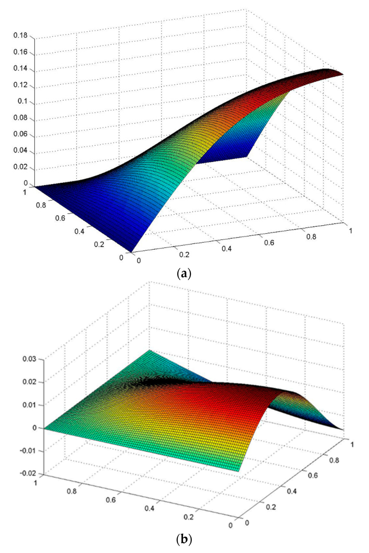
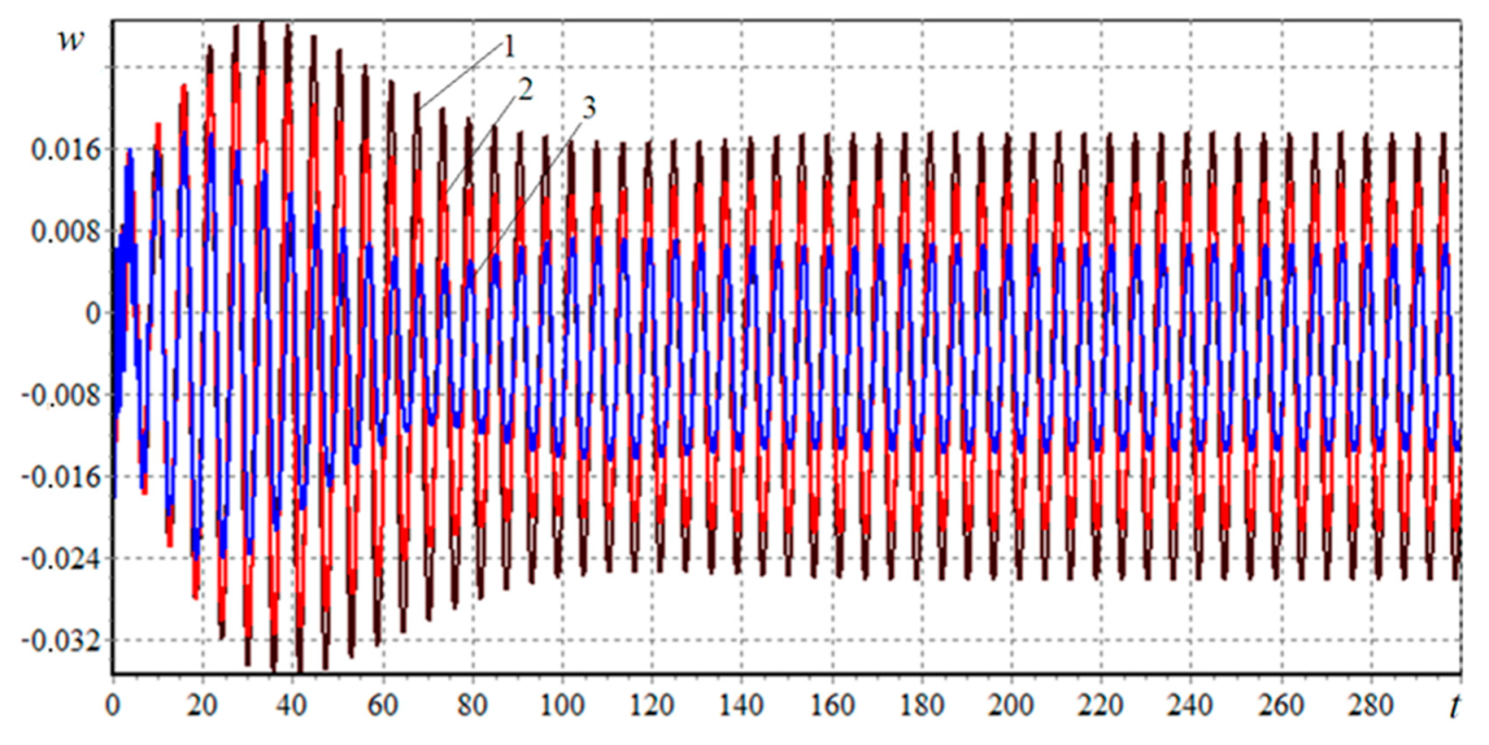
3.3.1. Behavior of the Plate versus Viscoelastic and Inhomogeneous Properties of the Material

The influence of the viscoelastic properties of the material on the behavior of the plate was studied. Figure 2 shows the time history of the deflection w for the following parameters: λ = 1, δ = 25, α* = 0.3, w₀ = 0.01, δ₀ = 0.3, δ₁ = 0.5, θ = 1.1, Δ = 1.2, μ₁ = 0.32, μ₂ = 0.27, and g = 0.3833.

The results show that taking into account the viscosity of the plate’s material leads to a decrease in the vibration amplitude obtained as a result of the calculation. At the initial moment, the amplitudes of the oscillations coincide. Then, over time, the results obtained in the elastic and viscoelastic formulations differ from each other by 40% or more.

Figure 3 shows the vibration modes of an elastic and viscoelastic rectangular plate.

Figure 4 shows the effect of inhomogeneous material properties of a viscoelastic plate on deflection at λ = 1, δ = 25, α* = 0.3, w₀ = 0.01, δ₀ = 0.3, δ₁ = 0.5, θ = 1.1, μ₁ = 0.32, μ₂ = 0.27, and g = 0.3833. Here, curve 1 is in the setting of the viscoelastic properties only along the shear directions, and curve 2 is in the setting of the viscoelastic properties in all directions. The results show that taking into account the plate material’s inhomogeneous properties leads to decreased vibration amplitude.

Figure 5 shows the vibration modes of a viscoelastic rectangular plate without considering the inhomogeneous properties of the plate material.

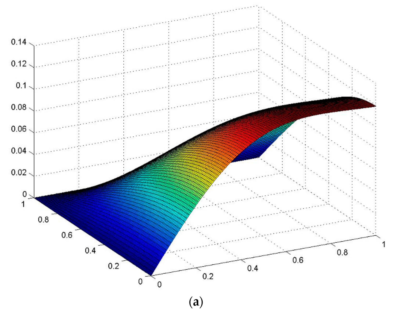
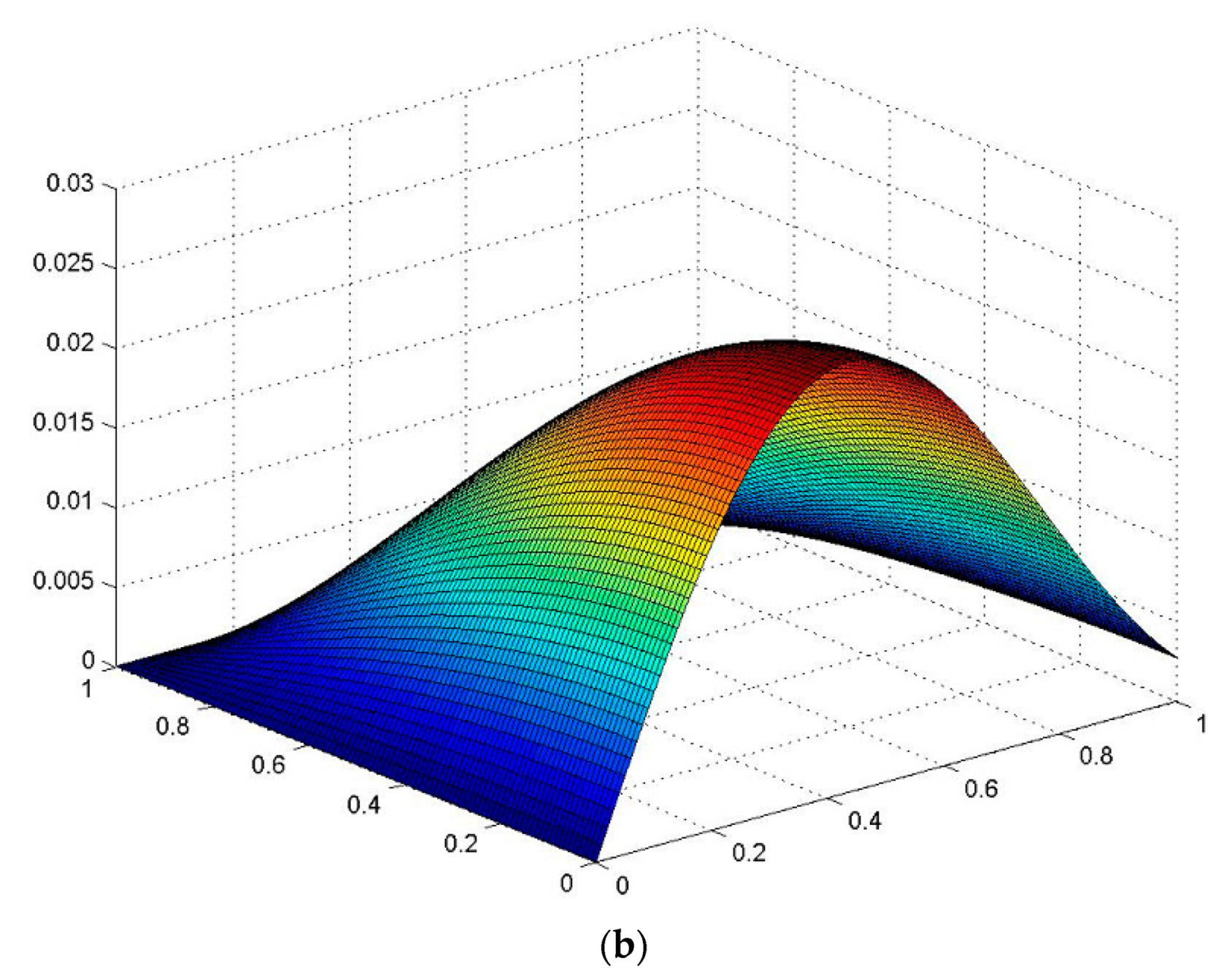
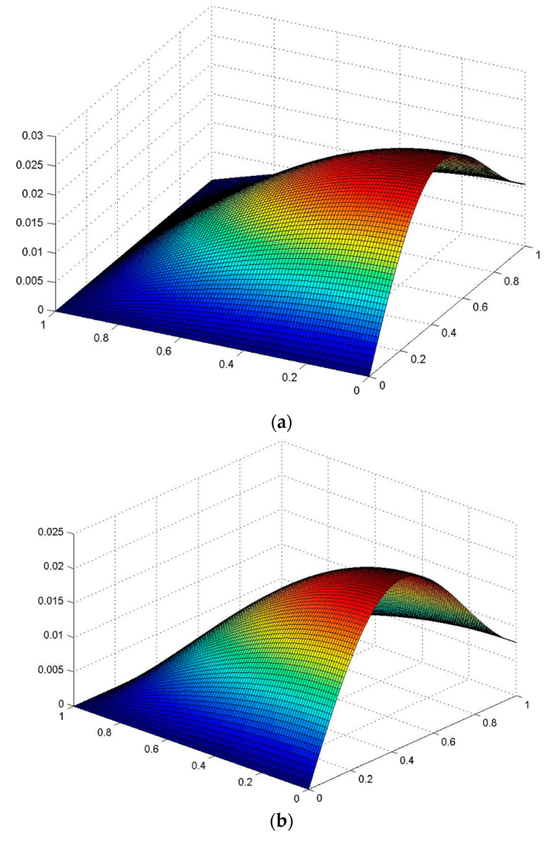
3.3.2. Behavior of the Plate at Various Thicknesses of the Plate

Figure 6 shows the change in the deflection of a viscoelastic plate as a function of time for different values of the thickness variability parameter ${\alpha }^{\ast }$ at λ = 1, δ = 25, A_ij = 0.05, w₀ = 0.01, δ₀ = 0.3, δ₁ = 0.5, θ = 1.1, Δ = 1.2, μ₁ = 0.32, μ₂ = 0.27, and g = 0.3833. It is seen that an increase in this parameter, i.e., a decrease in the plate’s stiffness, leads to a decrease in the vibration amplitude.

Figure 7 shows the vibration modes of a viscoelastic rectangular plate for various values of the thickness variability parameter.

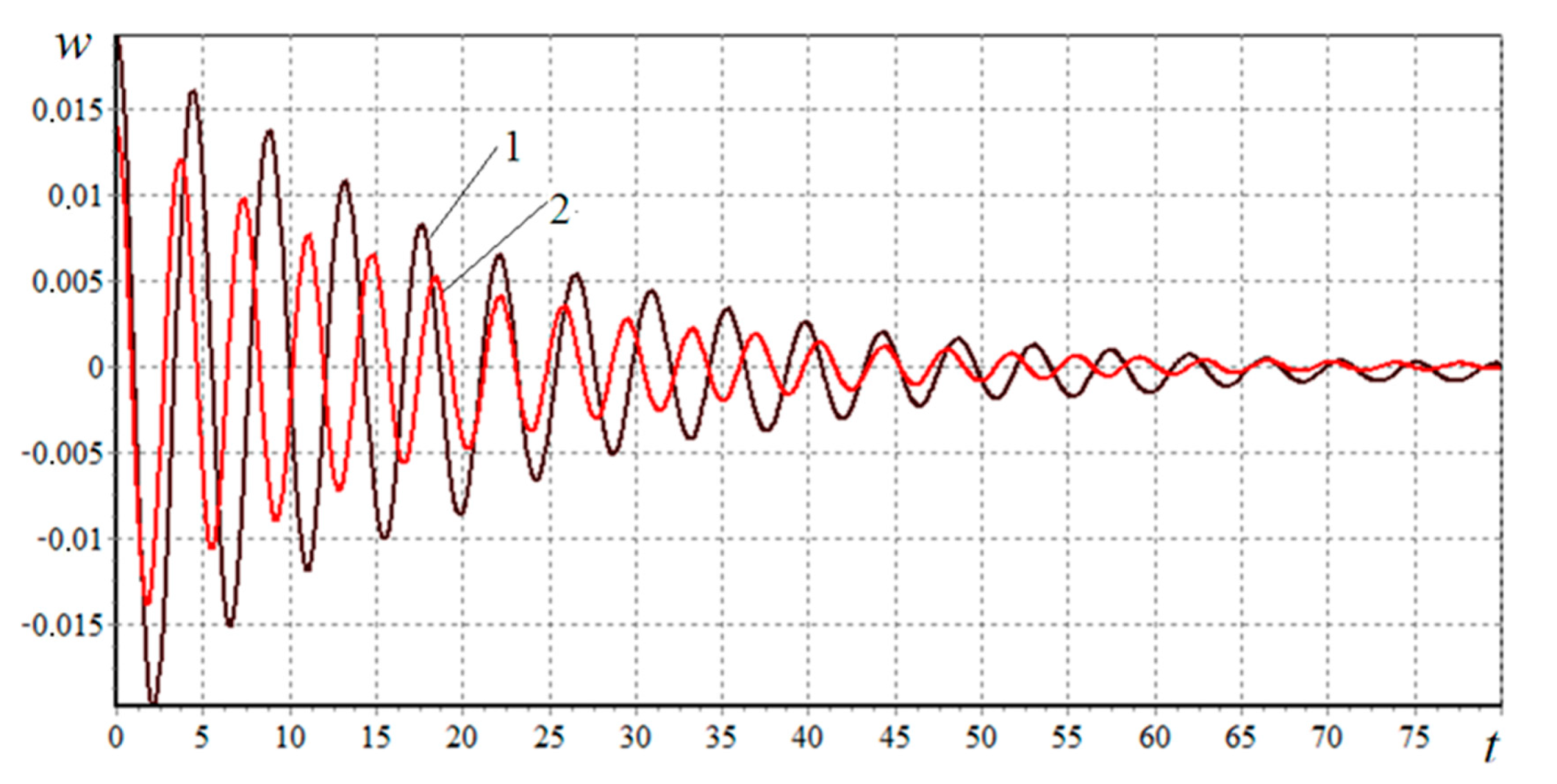
3.3.3. Behavior of the Plate at Various Boundary Conditions

Figure 8 shows the time dependence of the deflection of an orthotropic viscoelastic rectangular plate of variable thickness at λ = 1, δ = 25, α* = 0.3, q = 1, w₀ = 0.01, A_ij = 0.05, δ₀ = 0, δ₁ = 0.2, θ = 1.1, Δ = 1.2, μ₁ = μ₂ = 0.32, and g = 0.3833 for various boundary conditions: (1) two opposite sides are simply supported, and the other two are clamped; (2) all sides are clamped.

The results obtained show that, for given initial conditions and damping, with an increase in the plate’s number of clamped sides, the vibration amplitude decreases and the vibration frequency increases. In general, the results reflect the physical behavior of the considered plate vibrations. They are in qualitative agreement with the results obtained by the authors earlier [7,8,9,10,45,48].

It is of interest to compare the above results with the results obtained by the finite element method. It was noted above that such calculations are associated with significant computational and methodological difficulties. Of the publications found [51,52,53,54,55], only one publication provides a satisfactory possibility for the comparison. In [55], a finite element model based on the four-variable refined plate theory was used for forced vibration analysis of rectangular viscoelastic laminated composite plates integrated with a piezoelectric layer.

The piezoelectric layer acted as an actuator and was attached to the top surface of the plate. Comparison of the results obtained in this study with the results of [55] shows the following:

(i)

An increase in the stiffness of the plate (Figure 6) leads to a decrease in the vibration amplitude, which qualitatively agrees with the results of the work of Rouzegar and Davoudi ([55]).

(ii)

An increase in the number of clamped sides (Figure 8) leads to a decrease in the amplitude of oscillations and a phase shift to the left, which is also qualitatively consistent with the results of the work of Rouzegar and Davoudi ([55]).

The work of Rouzegar and Davoudi [55] is available in open access at https://link.springer.com/article/10.1007/s10409-020-00964-1 (accessed on 28 June 2021).

4. Conclusions

This study achieved the following results.

• The dynamic stability of an orthotropic viscoelastic rectangular plate of variable thickness, considering the geometric nonlinearity under the action of periodic loads, was described by a nonlinear system of integrodifferential equations.
• The application of Bubnov–Galerkin method, based on a polynomial approximation of the deflection and displacements, with the following discretization of spatial variables at each moment of time, reduces the problem of dynamic stability of an orthotropic viscoelastic rectangular plate of variable thickness to solving a nondecaying system of ordinary nonlinear integrodifferential equations with weakly singular kernels with variable coefficients.
• The proposed numerical method for solving a nondecaying system of nonlinear integrodifferential equations with variable coefficients with weakly singular kernels, using the algorithm for eliminating singularities of integrodifferential equations with a singular kernel of the Koltunov–Rzhanitsyn type, based on the use of quadrature formulas, is effective for solving problems of dynamic stability of orthotropic viscoelastic plates.
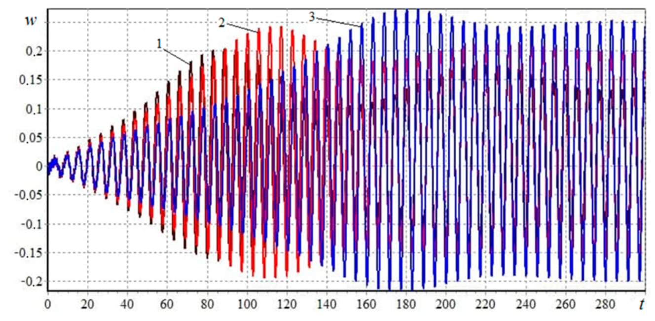
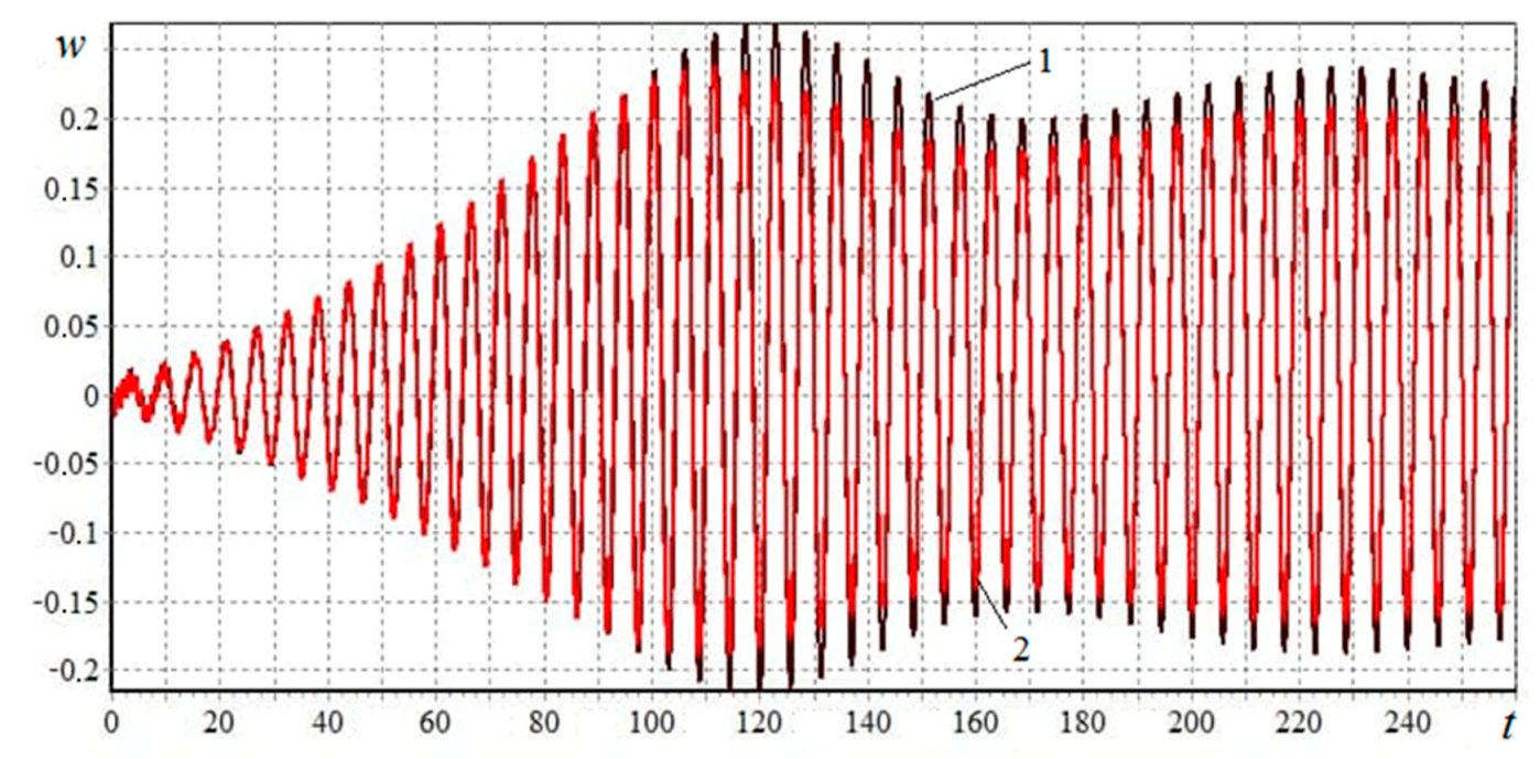
• It was found that an increase in the value of the rheological parameter α of the Koltunov–Rzhanitsyn core leads to an increase in the vibration amplitude. In this case, α plays an essential role in comparison with the parameter β. Parameter β has no significant effect on the change in the amplitude of the oscillation.
• It was found that the results of the viscoelastic problem obtained using the exponential relaxation kernel almost coincide with the results of the elastic problem. Using the Koltunov–Rzhanitsyn kernel, the differences between elastic and viscoelastic problems turn out to be very significant and amount to more than 40%.
• The proposed method can be used for various viscoelastic thin-walled structures such as plates, panels, and shells of variable thickness.
• The developed technique for studying vibrations of a viscoelastic orthotropic plate of variable thickness is easily extended to other types of laws of thickness variation, in the case of specifying in an analytical form the law of thickness variation in one or two directions of the coordinate axes.

References

1. Bolotin, V.V. The Dynamic Stability of Elastic Systems; Holden-Day: San Francisco, CA, USA, 1964; ISBN 978-1114366091. [Google Scholar]
2. Volmir, A.S. Stability of Deformable Systems; NASA AD-7169388; Defense Technical Information Center: Fort Belvoir, VA, USA, 1965.
3. Sahu, S.K.; Datta, P.K. Research Advances in the Dynamic Stability Behavior of Plates and Shells: 1987–2005—Part I: Conservative Systems. Appl. Mech. Rev. 2007, 60, 65–75. [Google Scholar] [CrossRef]
4. Amabili, M. Vibrations of Isotropic and Laminated Composite Circular Cylindrical Shells. In Nonlinear Mechanics of Shells and Plates in Composite, Soft and Biological Materials; Cambridge University Press: New York, NY, USA, 2018. [Google Scholar]
5. Amabili, M. Nonlinear Vibrations and Stability of Shells and Plates: Amabili; Marco: 9780521883290: Amazon.com: Books; Cambridge University Press: New York, NY, USA, 2018; ISBN 978-0521883290. [Google Scholar]
6. Alijani, F.; Amabili, M. Non-linear vibrations of shells: A literature review from 2003 to 2013. Int. J. Non-Linear Mech. 2014, 58, 233–257. [Google Scholar] [CrossRef] [Green Version]
7. Amabili, M. Nonlinear vibrations of viscoelastic rectangular plates. J. Sound Vib. 2016, 362, 142–156. [Google Scholar] [CrossRef]
8. Amabili, M. Nonlinear damping in nonlinear vibrations of rectangular plates: Derivation from viscoelasticity and experimental validation. J. Mech. Phys. Solids 2018, 118, 275–292. [Google Scholar] [CrossRef]
9. Amabili, M.; Balasubramanian, P.; Ferrari, G. Nonlinear vibrations and damping of fractional viscoelastic rectangular plates. Nonlinear Dyn. 2020. [Google Scholar] [CrossRef]
10. Balasubramanian, P.; Ferrari, G.; Amabili, M. Identification of the viscoelastic response and nonlinear damping of a rubber plate in nonlinear vibration regime. Mech. Syst. Signal Process. 2018, 111, 376–398. [Google Scholar] [CrossRef]
11. Lu, Y.; Shao, Q.; Amabili, M.; Yue, H.; Guo, H. Nonlinear vibration control effects of membrane structures with in-plane PVDF actuators: A parametric study. Int. J. Nonlinear Mech. 2020, 122, 103466. [Google Scholar] [CrossRef]
12. Darabi, M.; Ganesan, R. Nonlinear dynamic instability analysis of laminated composite thin plates subjected to periodic in-plane loads. Nonlinear Dyn. 2018, 91, 187–215. [Google Scholar] [CrossRef]
13. Huynh, H.Q.; Nguyen, H.; Nguyen, H.L.T. Non-linear parametric vibration and dynamic instability of laminated composite plates using extended dynamic stiffness method. J. Eng. Technol. 2017, 6, 170–185. [Google Scholar]
14. Souad, H.; Ismail, M.; Hichem, A.; Noureddine, E. Vibration analysis of viscoelastic fgm nanoscale plate resting on viscoelastic medium using higher-order theory. Period. Polytech. Civ. Eng. 2021, 65, 255–275. [Google Scholar] [CrossRef]
15. Kumar, R.; Dutta, S.C.; Panda, S.K. Linear and non-linear dynamic instability of functionally graded plate subjected to non-uniform loading. Compos. Struct. 2016, 154, 219–230. [Google Scholar] [CrossRef]
16. Kumar, R.; Mondal, S.; Guchhait, S.; Jamatia, R. Analytical approach for dynamic instability analysis of functionally graded skew plate under periodic axial compression. Int. J. Mech. Sci. 2017, 130, 41–51. [Google Scholar] [CrossRef]
17. Wu, H.; Yang, J.; Kitipornchai, S. Parametric instability of thermo-mechanically loaded functionally graded graphene reinforced nanocomposite plates. Int. J. Mech. Sci. 2018, 135, 431–440. [Google Scholar] [CrossRef] [Green Version]
18. Pirmoradian, M.; Torkan, E.; Karimpour, H. Parametric resonance analysis of rectangular plates subjected to moving inertial loads via IHB method. Int. J. Mech. Sci. 2018, 142–143, 191–215. [Google Scholar] [CrossRef]
19. Zhang, D.-B.; Tang, Y.-Q.; Chen, L.-Q. Internal resonance in parametric vibrations of axially accelerating viscoelastic plates. Eur. J. Mech. A Solids 2019, 75, 142–155. [Google Scholar] [CrossRef]
20. Kurpa, L.; Mazur, O.; Tkachenko, V. Parametric vibration of laminated plates with complex shape. In Proceedings of the Dynamical systems. Analytical/Numerical Methods, Stability, Bifurcation and Chaos, Łódź, Poland, 5–8 December 2011; pp. 289–294. [Google Scholar]
21. Awrejcewicz, J.; Kurpa, L.; Mazur, O. Dynamical instability of laminated plates with external cutout. Int. J. Nonlinear Mech. 2016, 81, 103–114. [Google Scholar] [CrossRef] [Green Version]
22. Kurpa, L.; Mazur, O.; Tkachenko, V. Dynamical stability and parametrical vibrations of the laminated plates with complex shape. Lat. Am. J. Solids Struct. 2013, 10, 175–188. [Google Scholar] [CrossRef] [Green Version]
23. Kurpa, L.V.; Mazur, O.S. Method of R-function for investigation of parametric vibrations of orthotropic plates of complex shape. J. Math. Sci. 2011, 174, 269. [Google Scholar] [CrossRef]
24. Kurpa, L.; Mazur, O.; Tkachenko, V. Investigation of the Parametric Vibrations of Laminated Plates by RFM. In Proceedings of the Proceedings of the 5 th International Conference on Nonlinear Dynamics, Kharkov, Ukraine, 27–30 September 2016. [Google Scholar]
25. Awrejcewicz, J.; Kurpa, L.; Mazur, O. On the Parametric Vibrations and Meshless Discretization of Orthotropic Plates with Complex Shape. Int. J. Nonlinear Sci. Numer. Simul. 2010, 11, 371–386. [Google Scholar] [CrossRef] [Green Version]
26. Kurpa, L.V.; Mazur, O.S.; Tkachenko, V.V. Parametric vibration of multilayer plates of complex shape. J. Math. Sci. 2014, 203, 165–184. [Google Scholar] [CrossRef] [Green Version]
27. Kurpa, L.V.; Mazur, O.S. Parametric vibrations of orthotropic plates with complex shape. Int. Appl. Mech. 2010, 46, 438–449. [Google Scholar] [CrossRef]
28. Chen, W.-R.; Chen, C.-S.; Shyu, J.-H. Stability of parametric vibrations of laminated composite plates. Appl. Math. Comput. 2013, 223, 127–138. [Google Scholar] [CrossRef]
29. Kosheleva, E. Dynamic stability of a viscoelastic plate. MATEC Web Conf. 2017, 117. [Google Scholar] [CrossRef] [Green Version]
30. Awrejcewicz, J.; Krys’ko, A.V. Analysis of complex parametric vibrations of plates and shells using Bubnov-Galerkin approach. Arch. Appl. Mech. 2003, 73, 495–504. [Google Scholar] [CrossRef]
31. Ramu, I.; Mohanty, S.C. Vibration and Parametric Instability of Functionally Graded Material Plates. J. Mech. Des. Vib. 2014, 2, 102–110. [Google Scholar] [CrossRef]
32. Eshmatov, B.K. Nonlinear vibrations and dynamic stability of viscoelastic orthotropic rectangular plates. J. Sound Vib. 2007, 300, 709–726. [Google Scholar] [CrossRef]
33. Eshmatov, B.K.; Eshmatov, K.; Khodzhaev, D.A. Nonlinear flutter of viscoelastic rectangular plates and cylindrical panels of a composite with a concentrated masses. J. Appl. Mech. Tech. Phys. 2013, 54, 578–587. [Google Scholar] [CrossRef]
34. Éshmatov, B.K. Nonlinear vibration analysis of viscoelastic plates based on a refined Timoshenko theory. Int. Appl. Mech. 2006, 42, 596–605. [Google Scholar] [CrossRef]
35. Éshmatov, B.K. Dynamic stability of viscoelastic plates under increasing compressing loads. J. Appl. Mech. Tech. Phys. 2006, 47, 289–297. [Google Scholar] [CrossRef]
36. Stojanović, V.; Petković, M.D.; Deng, J. Stability of parametric vibrations of an isolated symmetric cross-ply laminated plate. Compos. Part B Eng. 2019, 167, 631–642. [Google Scholar] [CrossRef]
37. Reddy, J.N. Theory and Analysis of Elastic Plates and Shells, 2nd ed.; CRC Press: Boca Raton, FL, USA, 2006; ISBN 9780429127601. [Google Scholar]
38. Rzhanicyn, A.R. Theory Creep; Stroyizdat: Moskow, Russia, 1968. [Google Scholar]
39. Elements of Hereditary Solid Mechanics, 1st ed.; MIR Publishers: Moscow, Russia, 1980; ISBN 978-0714714578.
40. Koltunov, M.A. Choice of kernels in solving problems involving creep and relaxation. Polym. Mech. 1966, 2, 303–311. [Google Scholar] [CrossRef]
41. Koltunov, M.A. Creep and Relaxation; Visshaya Shkola: Moscow, Russia, 1976. [Google Scholar]
42. Badalov, F.B. Methods for Solving Integral and Integro-Differential Equations of the Hereditary Theory of Viscoelasticity; Tashkent, P., Ed.; Mehnat: Tashkent, Uzbekistan, 1987. [Google Scholar]
43. Mirsaidov, M.M.; Abdikarimov, R.A.; Vatin, N.I.; Zhgutov, V.M.; Khodzhaev, D.A.; Normuminov, B.A. Nonlinear parametric oscillations of viscoelastic plate of variable thickness. Mag. Civ. Eng. 2018, 82, 112–126. [Google Scholar] [CrossRef]
44. Abdikarimov, R.; Khodzhaev, D.; Vatin, N. To Calculation of Rectangular Plates on Periodic Oscillations. MATEC Web Conf. 2018, 245. [Google Scholar] [CrossRef] [Green Version]
45. Normuminov, B.; Abdikarimov, R.; Khodzhaev, D.; Khafizova, Z. Parametric oscillations of viscoelastic orthotropic plates of variable thickness. In Proceedings of the IOP Conference Series: Materials Science and Engineering, Vladimir, Russia, 7–9 April 2020; Volume 896. [Google Scholar]
46. Volmir, A.S. The Nonlinear Dynamics of Plates and Shells; Foreign Technology Division Wright-Patterson Air Force: Dayton, OH, USA, 1974. [Google Scholar]
47. Ambartsumyan, S.A. Theory of Anisotropic Plates: Strength, Stability, & Vibrations; CRC Press: Boca Raton, FL, USA, 1991; ISBN 978-0891166542. [Google Scholar]
48. Abdikarimov, R.A.; Khodzhaev, D.A. Computer modeling of tasks in dynamics of viscoelastic thinwalled elements in structures of variable thickness. Mag. Civ. Eng. 2014, 49, 83–94. [Google Scholar] [CrossRef]
49. Mal’tsev, L.E. The analytical determination of the Rzhanitsyn-Koltunov nucleus. Mech. Compos. Mater. 1979, 15, 131–133. [Google Scholar] [CrossRef]
50. Courant, R. Differential and Integral Calculus, 2nd ed.; Wiley: New York, NY, USA, 1988; Volume 1, ISBN 978-0-471-60842-4. [Google Scholar]
51. Ray, M.C.; Mallik, N. Finite element analysis of smart structures containing piezoelectric fiber-reinforced composite actuator. AIAA J. 2004, 42, 1398–1405. [Google Scholar] [CrossRef]
52. Moita, J.S.; Araújo, A.L.; Mota Soares, C.M.; Mota Soares, C.A. Finite element model for damping optimization of viscoelastic sandwich structures. Adv. Eng. Softw. 2013, 66, 34–39. [Google Scholar] [CrossRef]
53. Wang, Y.Z.; Tsai, T.J. Static and dynamic analysis of a viscoelastic plate by the finite element method. Appl. Acoust. 1988, 25, 77–94. [Google Scholar] [CrossRef]
54. Rouzegar, J.; Abbasi, A. A refined finite element method for bending analysis of laminated plates integrated with piezoelectric fiber-reinforced composite actuators. Acta Mech. Sin. Xuebao 2018, 34, 689–705. Available online: https://link.springer.com/article/10.1007 (accessed on 28 June 2021). [CrossRef]
55. Rouzegar, J.; Davoudi, M. Forced vibration of smart laminated viscoelastic plates by RPT finite element approach. Acta Mech. Sin. 2020, 36, 933–949. [Google Scholar] [CrossRef]
Figure 1. An orthotropic viscoelastic rectangular plate of variable thickness under the action of periodic in-plane loads.
Applsci 11 06029 g001
Figure 2. Time history of the deflection w for (1) Aij = 0.01, (2) Aij = 0.02, and (3) Aij = 0.03.
Applsci 11 06029 g002
Figure 3. Vibration form of a rectangular plate of variable thickness at t = 78: (a) elastic at Aij = 0; (b) viscoelastic at Aij = 0.05.
Applsci 11 06029 g003aApplsci 11 06029 g003b
Figure 4. Dependence of the deflection on time: (1) Aij = 0.02, ⊗ = 1.1; (2) Aij = 0.02, ⊗ = 1.3.
Applsci 11 06029 g004
Figure 5. Vibration form of a rectangular plate of variable thickness at t = 180: (a) A, Aij = 0; (b) A, Aij = 0.05.
Applsci 11 06029 g005
Figure 6. Dependence of the deflection on time at (1) α* = 0.2, (2) α* = 0.5, and (3) α* = 0.8.
Applsci 11 06029 g006
Figure 7. Vibration form of a rectangular plate at t = 130: (a) α = 0; (b) α = 0.3.
Applsci 11 06029 g007
Figure 8. Dependence of the deflection on time for various boundary conditions: (1) two opposite sides are simply supported, and the other two are clamped; (2) all sides are clamped.
Applsci 11 06029 g008
Publisher’s Note: MDPI stays neutral with regard to jurisdictional claims in published maps and institutional affiliations.