
Semi-Quantitative Analysis of Major Elements and Minerals: Clues from a Late Pleistocene Core from Campos Basin

 , , ,
, , , 
Abstract
:1. Introduction
2. Materials and Methods
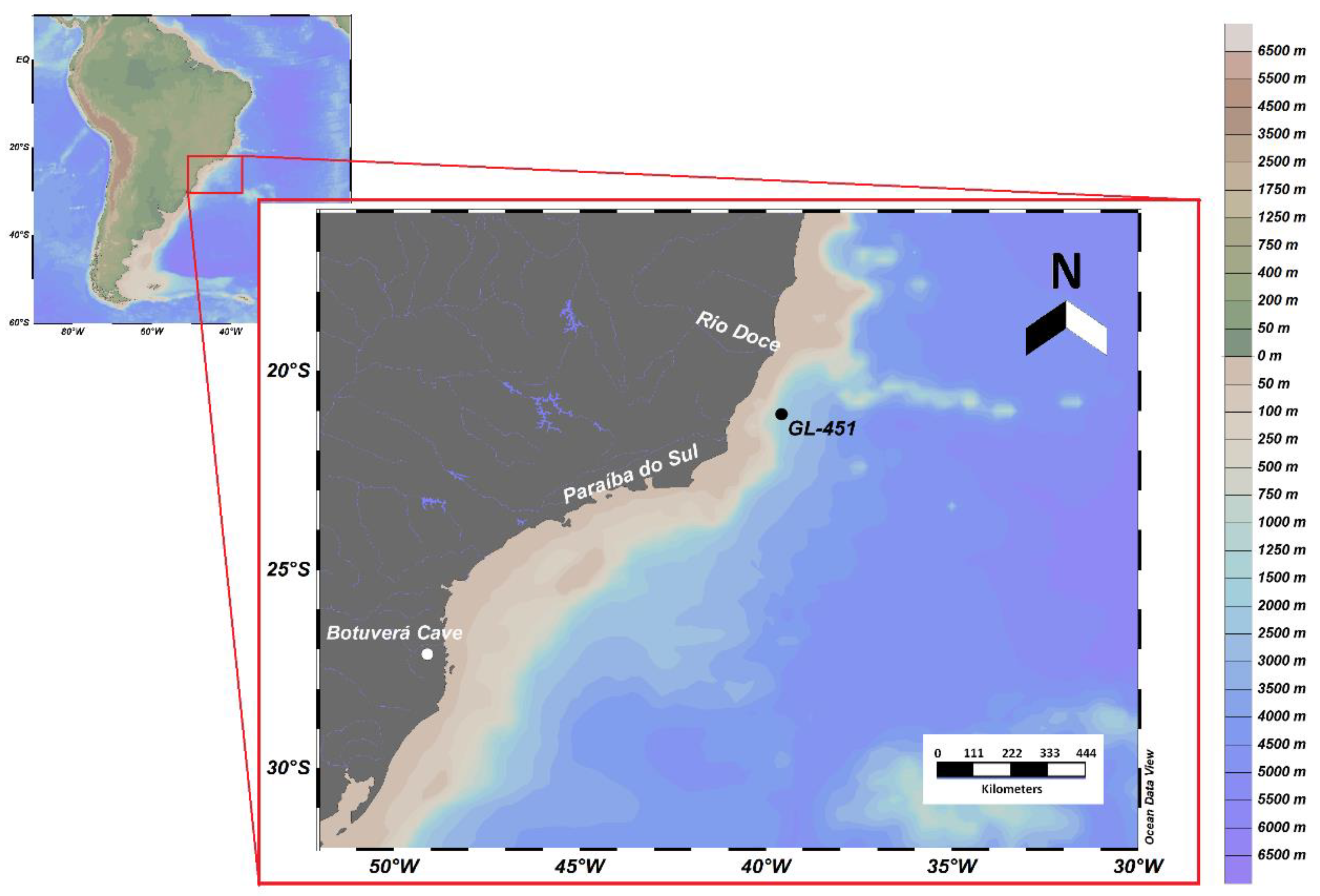
2.1. Marine Sediment Core
2.2. XRD and XRF Analysis
2.3. Data Analysis
3. Results
3.1. XRF Technique and Elementary Ratios
3.2. Mineralogical Composition of the Sediments
4. Discussion
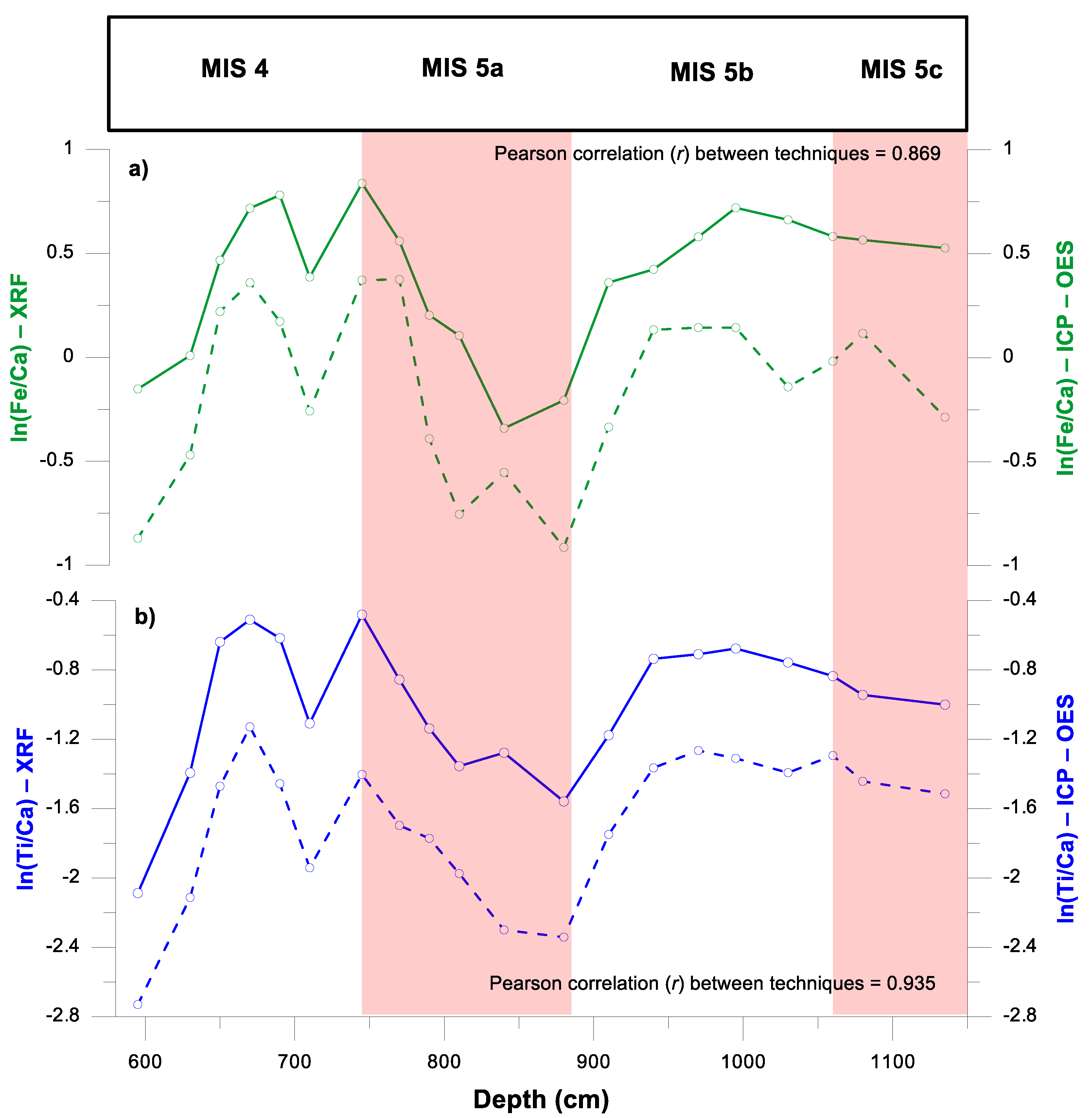
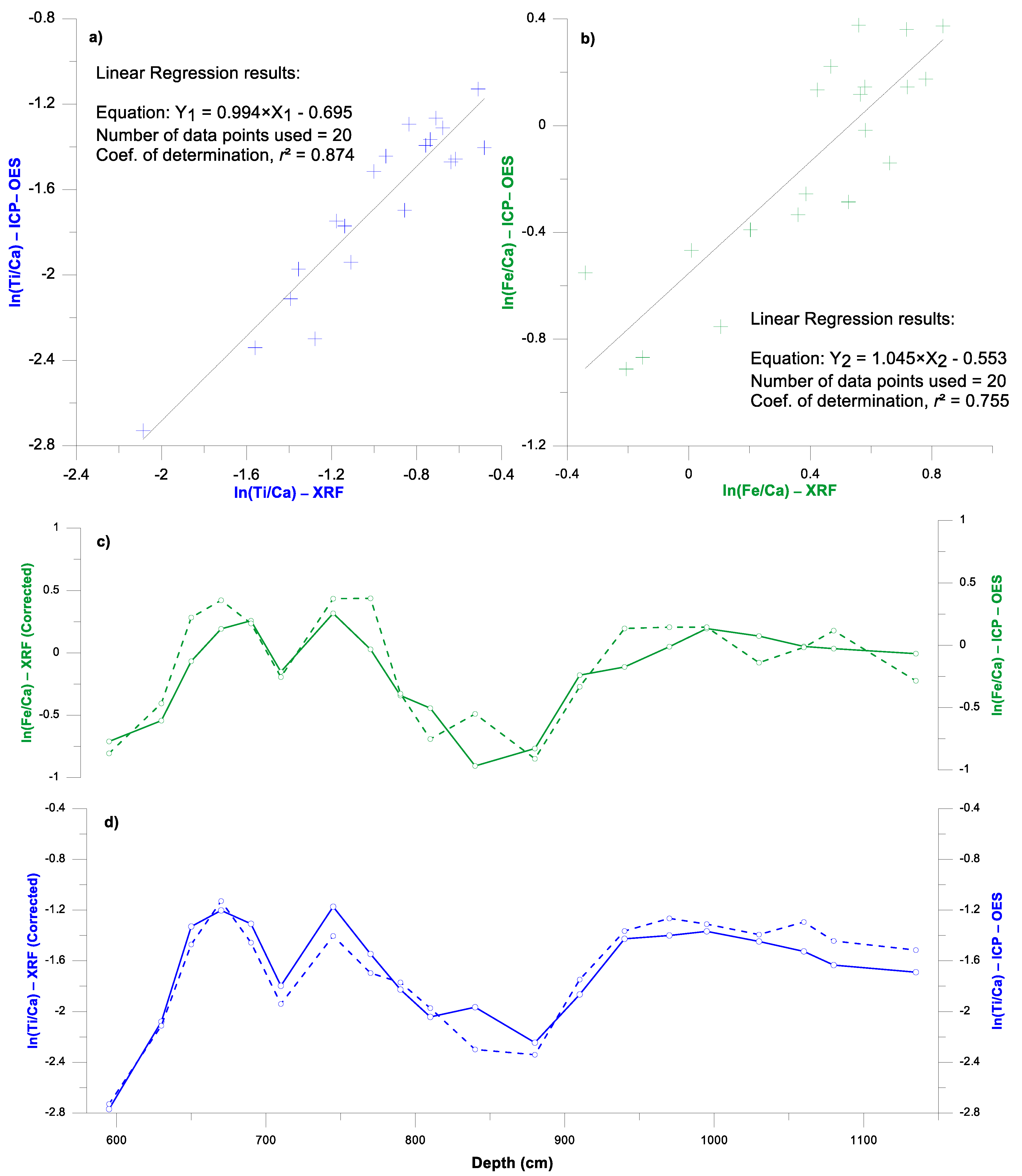
4.1. XRF Validation
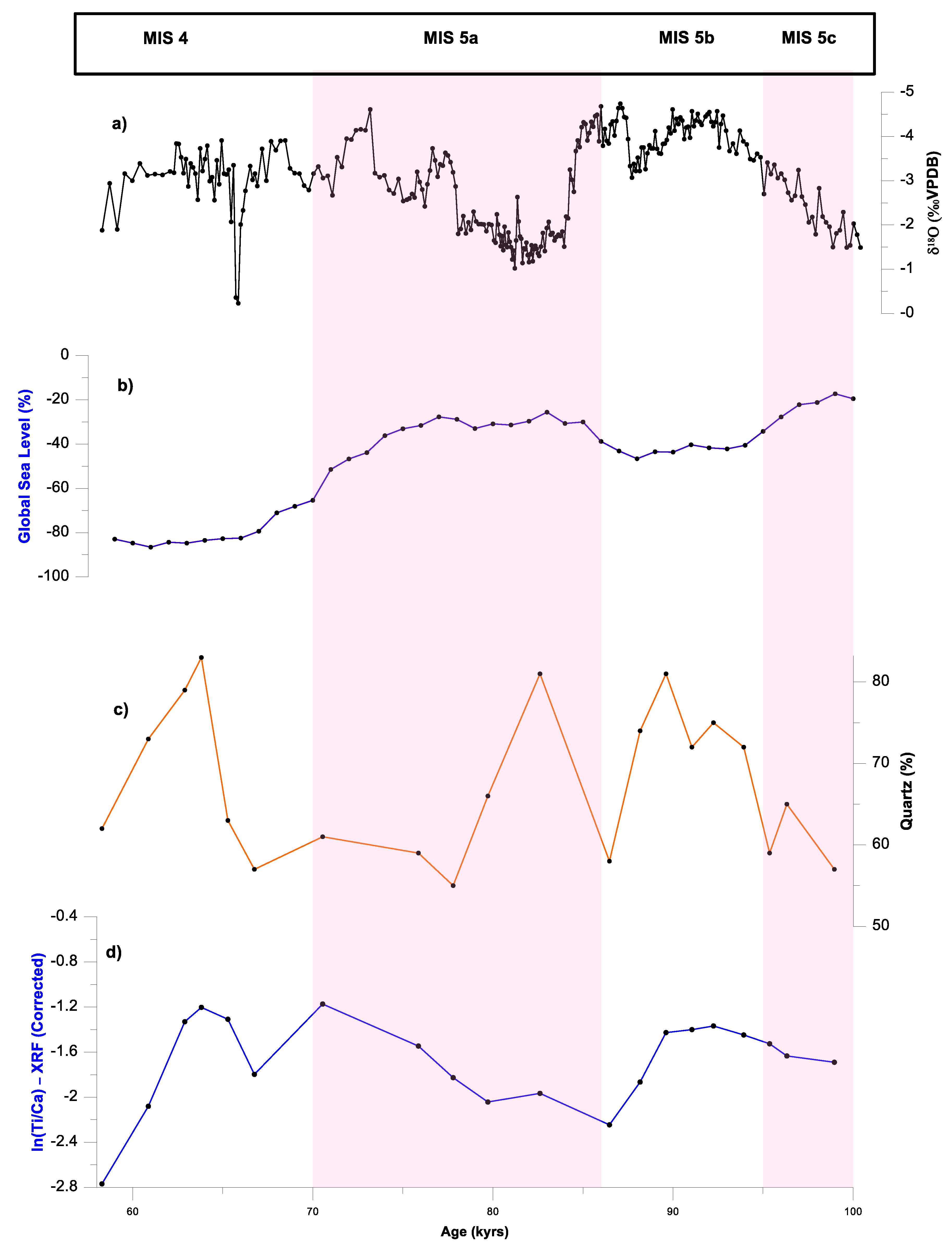
4.2. Paleoceanographic Application
5. Conclusions
Author Contributions
Funding
Institutional Review Board Statement
Informed Consent Statement
Data Availability Statement
Acknowledgments
Conflicts of Interest
References
- Arz, H.W.; Pätzold, J.; Wefer, G. Correlated millennial-scale changes in surface hydrography and terrigenous sediment yield inferred from last-glacial marine deposits off Brazil. Quat. Res. 1998, 50, 157–166. [Google Scholar] [CrossRef]
- Mahiques, M.M.; Tessler, M.G.; Ciotti, A.M.; Da Silveira, I.C.A.; e Sousa, S.H.D.M.; Figueira, R.C.L.; Tassinari, C.C.G.; Furtado, V.V.; Passos, R.F. Hydrodynamically driven patterns of recent sedimentation in the shelf and upper slope off Southeast Brazil. Cont. Shelf Res. 2004, 24, 1685–1697. [Google Scholar] [CrossRef]
- Luz, L.G.; Santos, T.P.; Eglinton, T.I.; Montluçon, D.; Ausin, B.; Haghipour, N.; Sousa, S.M.; Nagai, R.H.; Carreira, R.S. Contrasting late-glacial paleoceanographic evolution between the upper and lower continental slope of the western South Atlantic. Clim. Past 2020, 16, 1245–1261. [Google Scholar] [CrossRef]
- Araujo, L.D.; Lobo, F.J.; De Mahiques, M.M. The imprint of sedimentary processes in the acoustic structure of deposits on a current-dominated continental shelf. J. S. Am. Earth Sci. 2021, 105, 103005. [Google Scholar] [CrossRef]
- Behling, H.; Arz, H.W.; Pätzold, J.; Wefer, G. Late Quaternary vegetational and climate dynamics in northeastern Brazil: Inferences from marine core GEOB 3104-1. Quat. Sci. Rev. 2000, 19, 981–994. [Google Scholar] [CrossRef]
- Röhl, U.; Bralower, T.J.; Norris, R.D.; Wefer, G. New chronology for the late Paleocene thermal maximum and its environmental implications. Geology 2000, 28, 927–930. [Google Scholar] [CrossRef]
- Govin, A.; Holzwarth, U.; Heslop, D.; Keeling, L.F.; Zabel, M.; Mulitza, S.; Collings, J.A.; Chiessi, C.M. Distribution of major elements in Atlantic surface sediments (36° N–49° S): Imprint of terrigenous input and continental weathering. Geochem. Geophys. Geosyst. 2012, 13, 1–23. [Google Scholar]
- Weltje, G.J.; Tjallingii, R. Calibration of XRF core scanners for quantitative geochemical logging of sediment. Earth Planet. Sci. Lett. 2008, 274, 423–438. [Google Scholar] [CrossRef]
- Rothwell, R.G.; Rack, F.R. New Techniques in Sediment Core Analysis: An Introduction; Special Publication; Geological Society: London, UK, 2006; Volume 267, pp. 1–29. [Google Scholar]
- Boss, C.B.; Fredeen, K.J. Concepts, Instrumentation, and Techniques in Inductively Coupled Plasma Optical Emission Spectrometry; Perkin Elmer Corporation: Shelton, CT, USA, 1997. [Google Scholar]
- Stein, R.; Hefter, J.; Grützner, J.; Voelker, A.; Naafs, B.D.A. Variability of surface water characteristics and Heinrich-like events in the Pleistocene midlatitude North Atlantic Ocean: Biomarker and XRD records from IODP Site U1313 (MIS 16–9). Paleoceanography 2009, 24. [Google Scholar] [CrossRef]
- Li, J.; Liu, S.; Shi, X.; Zhang, H.; Fang, X.; Cao, P.; Yang, C.; Xue, X.; Khokiattiwong, S.; Kornkanitnan, N. Sedimentary responses to the sea level and Indian summer monsoon changes in the central Bay of Bengal since 40 ka. Marine Geol. 2019, 415, 105947. [Google Scholar] [CrossRef]
- Savian, J.F.; Jovane, L.; Frontalini, F.; Trindade, R.I.; Coccioni, R.; Bohaty, S.M.; Wilson, P.A.; Florindo, F.; Roberts, A.P.; Catanzariti, R.; et al. Enhanced primary productivity and magnetotactic bacterial production in response to middle Eocene warming in the Neo-Tethys Ocean. Palaeogeogr. Palaeoclimatol. Palaeoecol. 2014, 414, 32–45. [Google Scholar] [CrossRef]
- Savian, J.F.; Jovane, L.; Giorgioni, M.; Iacoviello, F.; Rodelli, D.; Roberts, A.P.; Chang, L.; Florindo, F.; Sprovieri, M. Environmental magnetic implications of magnetofossil occurrence during the Middle Eocene Climatic Optimum (MECO) in pelagic sediments from the equatorial Indian Ocean. Palaeogeogr. Palaeoclimatol. Palaeoecol. 2016, 441, 212–222. [Google Scholar] [CrossRef]
- Cornaggia, F.; Jovane, L.; Alessandretti, L.; Alves De Lima Ferreira, P.; Lopes Figueira, R.C.; Rodelli, D.; Berbel, G.B.B.; Braga, E.S. Diversions of the Ribeira River Flow and Their Influence on Sediment Supply in the Cananeia-Iguape Estuarine-Lagoonal System (SE Brazil). Front. Earth Sci. 2016, 6, 25. [Google Scholar] [CrossRef]
- Sarrazin, P.; Blake, D.; Feldman, S.; Chipera, S.; Vaniman, D.; Bish, D. Field Deployment of a Portable XRD/XRF Instrument on Mars Analog Terrain. Adv. X-ray Anal. 2005, 48, 194–203. [Google Scholar]
- Blake, D.; Vaniman, D.; Achilles, C.; Anderson, R.; Bish, D.; Bristow, T.; Chen, C.; Chipera, S.; Crisp, J.; Des Marais, D.; et al. Characterization and calibration of the CheMin mineralogical instrument on Mars Science Laboratory. Space Sci. Rev. 2012, 170, 341–399. [Google Scholar] [CrossRef] [Green Version]
- Costa, K.B.; Cabarcos, E.; Santarosa, A.C.A.; Battaglin, B.B.F.; Toledo, F.A.L. A multiproxy approach to the climate and marine productivity variations along MIS 5 in SE Brazil: A comparison between major components of calcareous nannofossil assemblages and geochemical records. Palaeogeogr. Palaeoclimatol. Palaeoecol. 2016, 449, 275–288. [Google Scholar] [CrossRef]
- Behling, H.; Arz, H.W.; Pätzold, J.; Wefer, G. Late Quaternary vegetational and climate dynamics in southwestern Brazil: Inferences from marine cores GEOB 3229-2 and GeoB 3202-1. Palaeogeogr. Palaeoclimatol. Palaeoecol. 2002, 179, 227–243. [Google Scholar] [CrossRef]
- Schlitzer, R. Ocean Data View, v.4.7.10. 2017. Available online: https://odv.awi.de/ (accessed on 30 June 2021).
- Wang, X.; Auler, A.S.; Edwards, R.L.; Cheng, H.; Cristalli, P.S.; Smart, P.L.; Richards, D.A.; Shen, C.C. Wet periods in northeastern Brazil over the past 210 kyr linked to distant climate anomalies. Nature 2004, 432, 740–743. [Google Scholar] [CrossRef]
- Degen, T.; Sadki, M.; Bron, E.; König, U.; Nénert, G. The highscore suite. Powder Diffr. 2014, 29, S13–S18. [Google Scholar] [CrossRef] [Green Version]
- Bland, J.M.; Altman, D.G. Applying the right statistics: Analyses of measurement studies. Ultrasound Obstet. Gynecol. 2003, 22, 85–93. [Google Scholar] [CrossRef]
- Melkonyan, G.A. A statistical comparison between the performance of ICP-OES and XRF methods for the analysis of trace amount of hg in urban soil samples. Electron. J. Nat. Sci. 2020, 34, 51–56. [Google Scholar]
- Balestra, B.; Rose, T.; Fehrenbacher, J.; Knobelspiesse, K.D.; Huber, B.T.; Gooding, T.; Paytan, A. In Situ Mg/Ca Measurements on Foraminifera: Comparison Between Laser Ablation Inductively Coupled Plasma Mass Spectrometry and Wavelength-Dispersive X-Ray Spectroscopy by Electron Probe Microanalyzer. Geochem. Geophys. Geosyst. 2021, 22. [Google Scholar] [CrossRef]
- Hammer, Ø.; Harper, D.A.; Ryan, P.D. PAST: Paleontological statistics software package for education and data analysis. Palaeontol. Electron. 2001, 4, 9. [Google Scholar]
- Geider, R.J.; La Roche, J. The role of iron in phytoplankton photosynthesis, and the potential for iron-limitation of primary productivity in the sea. Photosynth. Res. 1994, 39, 275–301. [Google Scholar] [CrossRef]
- Taylor, K.G.; Macquaker, J.H.S. Iron Minerals in Marine Sediments Record Chemical Environments. Elements 2011, 7, 113–118. [Google Scholar] [CrossRef]
- Hutton, J.T. Minerals in Soil Environment; Dixon, J.B., Weed, S.B., Eds.; Soil Science Society of America: Madison, WI, USA, 1977. [Google Scholar]
- Correns, C.W.; Wedepohl, K.H. (Eds.) Handbook of Geochemistry; Springer: Berlin, Germany, 1969; Volume 2. [Google Scholar]
- Wei, G.; Liu, Y.; Li, X.; Shao, L.; Liang, X. Climatic impact on Al, K, Sc and Ti in marine sediments: Evidence from ODP Site 1144, South China Sea. Geochem. J. 2003, 37, 593–602. [Google Scholar] [CrossRef] [Green Version]
- Sun, G.; Wang, Y.; Guo, J.; Wang, M.; Jiang, Y.; Pan, S. Clay Minerals and Element Geochemistry of Clastic Reservoirs in the Xiaganchaigou Formation of the Lenghuqi Area, Northern Qaidam Basin, China. Minerals 2019, 9, 678. [Google Scholar] [CrossRef] [Green Version]
- Cruz, F.W., Jr.; Burns, S.J.; Karmann, I.; Sharp, W.D.; Vuille, M.; Cardoso, A.O.; Ferrari, J.A.; Silva-Dias, P.L.; Viana, O., Jr. Insolation-driven changes in atmospheric circulation over the past 116,000 years in subtropical Brazil. Nature 2005, 434, 63–66. [Google Scholar] [CrossRef]
- Spratt, R.M.; Lisiecki, L.E. A Late Pleistocene sea level stack. Clim. Past 2016, 12, 1079–1092. [Google Scholar] [CrossRef] [Green Version]
- Leite, Y.L.; Costa, L.P.; Loss, A.C.; Rocha, R.G.; Batalha-Filho, H.; Bastos, A.C.; Quaresma, V.S.; Fagundes, V.; Passamani, M.; Pardini, R. Neotropical forest expansion during the last glacial period challenges refuge hypothesis. Proc. Natl. Acad. Sci. USA 2016, 113, 1008–1013. [Google Scholar] [CrossRef] [Green Version]
- Nace, T.E.; Baker, P.A.; Dwyer, G.S.; Silva, C.G.; Rigsby, C.A.; Burns, S.J.; Giosan, L.; Otto-Bliesner, B.; Liu, Z.; Zhu, J. The role of North Brazil Current transport in the paleoclimate of the Brazilian Nordeste margin and paleoceanography of the western tropical Atlantic during the late Quaternary. Palaeogeogr. Palaeoclimatol. Palaeoecol. 2014, 415, 3–13. [Google Scholar] [CrossRef]
- Gu, F.; Zonneveld, K.A.; Chiessi, C.M.; Arz, H.W.; Pätzold, J.; Behling, H. Long-term vegetation, climate and ocean dynamics inferred from a 73,500 years old marine sediment core (GeoB2107-3) off southern Brazil. Quat. Sci. Rev. 2017, 172, 55–71. [Google Scholar] [CrossRef]


| ln (Ti/Ca) | ln Fe/Ca | |||
|---|---|---|---|---|
| XRF | ICP-OES | XRF | ICP-OES | |
| Min | −2.087 | −2.733 | −0.341 | −0.911 |
| Max | −0.481 | −1.130 | 0.837 | 0.376 |
| Mean | −0.993 | −1.683 | 0.389 | −0.146 |
| Std. Error | 0.090 | 0.096 | 0.077 | 0.092 |
| Variance | 0.162 | 0.183 | 0.118 | 0.171 |
| Stand. dev | 0.402 | 0.428 | 0.344 | 0.413 |
| Shapiro–Wilk W | 0.924 | 0.906 | 0.913 | 0.924 |
| p (normal) | 0.117 | 0.053 | 0.072 | 0.118 |
Publisher’s Note: MDPI stays neutral with regard to jurisdictional claims in published maps and institutional affiliations. |
© 2021 by the authors. Licensee MDPI, Basel, Switzerland. This article is an open access article distributed under the terms and conditions of the Creative Commons Attribution (CC BY) license (https://creativecommons.org/licenses/by/4.0/).
Share and Cite
Pedrão, G.A.; Costa, K.B.; Toledo, F.A.L.; Tomazella, M.O.; Jovane, L. Semi-Quantitative Analysis of Major Elements and Minerals: Clues from a Late Pleistocene Core from Campos Basin. Appl. Sci. 2021, 11, 6206. https://doi.org/10.3390/app11136206
Pedrão GA, Costa KB, Toledo FAL, Tomazella MO, Jovane L. Semi-Quantitative Analysis of Major Elements and Minerals: Clues from a Late Pleistocene Core from Campos Basin. Applied Sciences. 2021; 11(13):6206. https://doi.org/10.3390/app11136206
Chicago/Turabian StylePedrão, Guilherme A., Karen B. Costa, Felipe A. L. Toledo, Mariana O. Tomazella, and Luigi Jovane. 2021. "Semi-Quantitative Analysis of Major Elements and Minerals: Clues from a Late Pleistocene Core from Campos Basin" Applied Sciences 11, no. 13: 6206. https://doi.org/10.3390/app11136206
APA StylePedrão, G. A., Costa, K. B., Toledo, F. A. L., Tomazella, M. O., & Jovane, L. (2021). Semi-Quantitative Analysis of Major Elements and Minerals: Clues from a Late Pleistocene Core from Campos Basin. Applied Sciences, 11(13), 6206. https://doi.org/10.3390/app11136206