Article

DR-Transformer: A Multi-Features Fusion Framework for Tropical Cyclones Intensity Estimation

1
School of Artificial Intelligence, Beijing University of Posts and Telecommunications, Beijing 100876, China
2
National Meteorological Center, Beijing 100081, China
*
Author to whom correspondence should be addressed.
Appl. Sci. 2021, 11(13), 6208; https://doi.org/10.3390/app11136208
Submission received: 29 April 2021 / Revised: 29 June 2021 / Accepted: 1 July 2021 / Published: 5 July 2021
(This article belongs to the Section Computing and Artificial Intelligence)

Abstract

:
Convolutional neural networks have achieved great success in analyzing potential features inside tropical cyclones (TCs) using satellite images for intensity estimation. However, due to the high similarity of visual features in TC images, it is still a challenge to learn the accurate mapping between TC images and numerical intensity. Existing works mainly focus on the visual features of a single TC, ignoring the impact of intensity continuity and time evolution among TCs on decision making. Therefore, we propose a DR-transformer framework for temporal TC intensity estimation. Inside DR-transformers, a novel DR-extractor can extract Distance-consistency(DC) and Rotation-invariance (RI) features between TC images, and therefore can better learn the contours, structures, and other visual features of each TC image. DC features can reduce the estimation error between adjacent intensities, and RI features can eliminate feature deviation caused by shooting angles and TC rotation. Additionally, a transformer with a DR-extractor as the backbone is applied to aggregate the temporal correlation in a series of TC images, which can learn the evolution from intensity to the visual features of TC. Experiments show that the final result, an RMSE of 7.76 knots, outperforms the baseline, and is better than any previously reported method trained on the TCIR dataset.

1. Introduction

Tropical cyclone (TC) intensity estimation is an image-to-intensity problem and has attracted much attention in recent years since it is significant in disaster warning or management. TC intensity, which is defined as the maximum sustained surface wind near the TC center, is the most important parameter that needs to be accurately estimated. A major challenge of this task is that the differences in TC visual features are small, especially for similar intensities, which often results in larger errors.
The conventional method for intensity estimation in past years is the Dvorak technique [1], which involves a human-constructed feature pattern and is subjective. Recently, approaches based on deep learning for TC intensity estimation have obtained increasing attention. The latest classification methods [2] estimate TC intensity by treating each intensity as an independent fixed class and use the cross-entropy loss to optimize the model. Regression methods [3,4] estimate exact intensity values of TCs by using mean squared error (MSE) as a loss function, reaching an RMSE of 8.39 knots in the TCIR dataset. Both classification and regression methods outperform manual intensity estimation methods. However, all these previous methods neglect a key point of intensity estimation, which is that TC that have similar feature patterns tend to have a closer intensity [1]. On the other hand, estimating intensity from only one image is not enough. Therefore, it is necessary to combine historical information and multi-view information. In [3], a five-point weighted average method was used to combine historical information. Although it shows an improvement in results, it did not consider the complicated relationship between temporal TC images. Another method proposed in [3] is to blend the estimations of images rotated by different angles to reduce the variance of estimation, which ignored multi-view features of the image itself.
Specifically, we describe our idea in Figure 1, where DC is short for distance-consistency, and RI is short for rotation-invariance. As shown in Figure 1a, existing methods reduce number of the negative samples, which caused samples with a larger intensity difference to have a relatively small distance difference. For example, if the intensity is 120, it can be misclassified into 80, which is unacceptable. However, in Figure 1b, it shows a perfect mapping between image and intensity; even if misclassified, it will only be done so to adjacent categories. Additionally, since TC is constantly rotating, it is important to extract rotation-invariance features. In Figure 1c, TCs are misclassified at certain camera angles, while their rotation-invariance features can be correctly classified. Here, we give two definitions. DC: distance-consistency—the equal proportion relationship between the sample intensity and sample distance in feature space. RI: rotation-invariance—the same TC images with different angles have the same representation in the feature space.
Motivated by the above, we formulated TC intensity estimation from a metric learning perspective and propose a DR-transformer framework with a DR-extractor and a transformer. The DR-extractor is a CNN model based on a joint loss of both Distance-consistency (DC) loss and Rotation-invariance (RI) loss. DC loss learned features by restraining the ratio, which is defined as the quotient of the differences in distance and in intensity. RI loss is used to extract the rotation-invariance feature according to the characteristics of continuous rotation of TC and differences in shooting perspectives. For extracting the RI feature, we ensured the feature embedding extracted from an image and its random-rotated counterpart were close. Finally, we applied a transformer [5] to aggregate the temporal correlation from a series of TC images, which can learn about the relationship between the change in intensity and that of TC contour, structure, and other visual features.
We further feed the extracted feature of our DR-transformer framework into a nearest neighbor (NN) classifier for estimating and predicting intensity. Extensive experiments on the TCIR [4] dataset demonstrate the effectiveness of our proposed method.
We summarize our contributions as follows:
  • We propose a distance-consistency loss function, which is a general loss function, especially suitable for constructing image features with continuous labels.
  • We apply a transformer for aggregating temporal correlation features, which is a multi-task model to make a better effect in the estimation and prediction of TC intensity.
  • Extensive experiments on the TCIR dataset demonstrate the effectiveness of our proposed approach, which outperforms the existing methods.

2. Related Works

2.1. Tropical Cyclone Intensity Estimate

There have been studies using CNN to estimate TC intensity [2,3,4,6]. As far as we know, the application of CNN to TC intensity estimation was first introduced by [2] and they classify TC images into eight classes. However, they just obtain intensity range instead of exact intensity, and their training data and test data are related. In [3,4], multi-channel satellite images and external information, such as latitude, longitude, and date, are used to estimate an exact intensity by a regression network. In [6], a context-aware cycleGAN was used to solve the problem of highly imbalanced TC data. In [7], GAN is used to generate PMW and VIS channel images from IR1 and WV channels for real-time TC intensity estimation.
However, existing methods suffer from a lack of interpretability and fail to make full use of the TC intensity (label), which are continuous and important to optimize an embedding space. Differently, our proposed DR-transformer framework considers TC estimation as a nearest neighbor classification problem and utilizes the continuity of labels to construct a distance-consistency embedding space in which we can easily find the neighbors of query image by the K-nearest neighbor classifier [8].

2.2. Metric Learning

A siamese network [9,10,11] is a representative method that learns embedding via contrastive loss based on pairs. It pushes samples from a negative pair apart from each other and encourages samples from a positive pair to be closer in the embedding space. In [12,13], triplet loss is introduced by using triplets as samples, which consist of a positive, a negative, and an anchor. Triplet loss aims to learn an embedding space where the distance of negative pairs is higher than that of positive pairs by giving a margin. Extended from above, N-pair loss [14], which takes anchor, positive, and N-2 negative samples as its input, and optimizes their embedding jointly. Circle loss [15] generalizes the above losses to a united formulation and can be applied to the circumstance of multi-positive pairs.
Recently, [16] proposed log-ratio loss, an improved triplet loss to handle continuous labels and optimize an embedding space where distance ratio can be preserved. However, their method can only be applied to triplets and uses structural annotation to obtain continuous labels, which is easily influenced by shooting angle. We move a step forward and propose a DC loss that can be applied to N-tuple and achieves excellent results.

2.3. Transformer

Transformer [5] is a new attention-based building block for machine translation. It can look through each element of a sequence and update it by combining information from the whole sequence. The transformer becomes pervasive and has made a tremendous impact in many fields such as language understanding [17,18,19] and image processing [20,21,22,23]. DETR [23] adopt transformers to object detection task and simplify the hand-crafted anchor matching procedure in object detection training. A vision transformer [21] divides an image into 16 × 16 patches and feeds these patches into a standard transformer. They directly utilize a transformer instead of CNN to extract low-level features such as dense, repeatable patterns. A visual transformer [22] uses convolutions for extracting low-level features and transformers for relating high-level concepts by spatial attention. Different from the above, we totally leverage convolutions to extract features and we further make use of the effectiveness of transformers to relate temporal features. We use temporal attention to refine feature embedding extracted from a sequence of images, aiming to obtain a stable estimation for intensity.

3. Methods

We illustrate the overall diagram of our framework in Figure 2, in which the top part is the training stage and the bottom part is the inference stage. During the training stage, our model can be trained in two steps. Firstly, we train a DR-extractor to obtain an adaptable and discriminative feature prototype. Secondly, we train a transformer by feeding the learned feature into the transformer sequentially to capture the temporal correlation. To complete the training process, we combined three properties of TC: distance consistency, rotation invariance, and temporal correlation. We will elaborate on these in the following paragraphs.
Formally, given a training dataset X = [ x 1 , x 2 , . . . ] of images x i R 1 × H × W and the corresponding ground-truth Y = [ y 1 , y 2 , . . . ] of label y i R + , our goal is to learn about an image representation f : x f ( x , θ ) R d in the form of the CNN with parameters θ . Then, the intensity can be estimated by Euclidean distance-based nearest neighbor classifier [8].

3.1. Image-to-Intensity Feature Learning

As shown in the top of Figure 2, we first trained a DR-extractor based on two principles: distance consistency and rotation invariance. The overall loss of our DR-extractor can be written as:
= D C + α R I
where D C is DC loss, R I is RI loss and α = 1 is a parameter to balance the contribution of different loss.

3.1.1. Distance Consistency Feature Learning

TC intensity in the dataset is a series of scalars and is different from traditional classify-based labels, which are discrete. If we treat continuous labels as discrete class labels or relative labels, we will neglect their numerical relations. Therefore, inspired by Kim [16], we proposed DC loss based on (N + 1)-tuplet in order to make full use of numerical relation. With the help of DC loss, we can construct a DC embedding space in which the distance between samples in the embedding space is directly proportional to that in the label space.
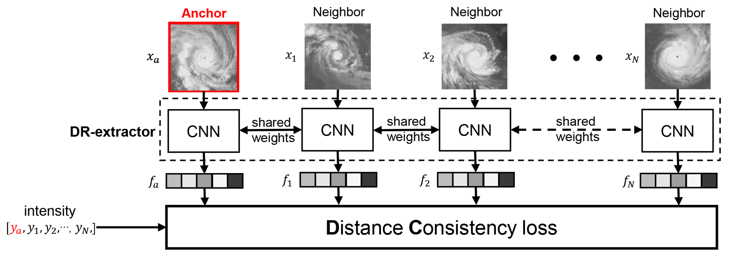
The training details of DC loss are shown in Figure 3. To obtain DC loss, we constructed a (N + 1)-tuplet of training samples with an anchor a and N neighbors randomly sampled from the remaining ones. Then we fed them into the CNN to obtain its embedding f ( x i , θ ) , hereinafter abbreviated to f i . Note that embedding f should be L 2 normalized because without such a normalization, their magnitudes tend to diverge. Then, for samples i and j, we defined pairwise ratios of feature embedding distance and label distance as
r i j = D ( f i , f j ) D ( y i , y j )
where D ( · ) indicates Euclidean distance. Finally, our distance-consistency loss can be formulated as
D C = i = 1 N log r a i j = 1 N r a j
where r a i / j = 1 N r a j is the normalization of r a i and a represents the anchor. Note that (3) reaches the minimum value while ratio r a 1 = r a 2 = . . . = r a N . Our loss aims to compare the ratio, which can reflect the consistency between label distance and feature embedding distance, to decide optimizing direction. Ideally, we hope the ratio between image pairs is almost equivalent and this property can be explained through its gradients, which are given by
D C f i = f i f a D ( f i , f a ) · i
D C f a = i = 1 N D C f i
where f i f a is a vector and i is a scalar value computed by
i = 1 r a i 1 N j = 1 N r a j
As shown in (4) and (5), the optimization of f i depends on both vector f i f a and scalar i . The former represents the direction between the embedding vectors and the latter compares different distance ratios with the mean value in a mini-batch to decide the optimizing direction to be the same or opposite. As shown in (6), if the ratio r a i is less than the mean of all the ratios, the scalar i is negative. Apparently, the distance of samples i , a that are close in label space will be pulled closer.
In the training stage, we utilized methods such as [14] to construct a mini-batch. We randomly select N samples as neighbors and M samples as anchors to construct mini-batch. Each anchor is combined with the N neighbors to form (N + 1)-tuplets because we find that all of the tuplets sharing the same neighbors lead to a more definite convergence status. Therefore, there are M tuplets in a mini-batch in total. Then, we fed the the mini-batch into the DR-extractor to obtain the feature embedding and then calculated the DC loss based on M tuplets.

3.1.2. Rotation-Invariance Feature Learning

TC is a complex and dynamic system with continuous rotation. Although its shape also changes slightly during the process of rotation, its characteristics and intensity are often constant. Therefore, it is more meaningful to the extract rotation-invariance feature than the general image recognition tasks. The idea of rotation invariance is that the feature embedding extracted from x and its randomly rotated counterpart x r should be close. Hence, we follow the common practice in semi-supervised learning to achieve this.
Formally, an image x rotated by r degrees is denoted as x r and r R = { 0 , 90 , 180 , 270 } is an angle selected from a set of possible angles. Then, the feature prototype is defined as
f ¯ = 1 | R | r R f ( x r )
We further use the mean squared error as RI loss, which is given by
r i = r R M S E ( f ( x r ) , f ¯ )
The goal of the rotation-invariance loss is that the feature of an image and its rotated copies are expected to be similar as much as possible. We solved this by minimizing the distance between each feature f ( x r ) and feature prototype f ¯ . The feature prototype is a fusion of the essential feature of the rotating TC and we further fed it to the transformer.
That means our DC embedding leads to fewer errors and is more adaptable to TC intensity estimations.

3.2. Temporal Correlation Learning via Transformer

It is necessary to utilize temporal information to estimate intensity. As using an image alone is not enough to estimate intensity accurately, there still exists unacceptable errors in some samples. TC intensity at a certain moment relates to the intensities before; learning the temporal correlation of TC is important for remedying results. To achieve this goal, we use the attention mechanism and transformer model.
Transformer structure: As shown in Figure 2, our transformer has a standard structure and mainly consists of multi-head self-attention modules, feed-forward networks, and cross-attention modules. N E and N G are the numbers of encoders and decoders, respectively. Regarding the self-attention of the transformer, we take the input as a query, key, and value. In cross-attention, the outputs from the encoder are regarded as a query and the outputs from decoder self-attention are taken as a query and value. We added fixed positional encodings to the input of each attention layer to record temporal information. To ensure estimation at moment t can only depend on the known estimation before moment t, we offset the input of the decoder by one position and mask (setting to ) the attention weights matrix of the decoder. For a sequence of length 4, the decoder weight mask is given by
D w e i g h t s ( i , j ) = 1 , if   i < = j inf , if   i > j
where blank means we offset the input of the decoder by one position and “-inf” means the weights in that position are masked.
Class vectors: we first utilized the DR-extractor to extract features from the whole training dataset and averaged the features by class (intensity) to construct a global class representation set C = { c 1 , c 2 , . . . } . The class vectors were used to train the transformer and for classification.
Training transformer: For the training transformer, we needed time series data and class vectors C. We selected a sequence of images and their corresponding intensities from a TC. Then, we utilized the DR-extractor to obtain the discriminative feature embedding of images and, meanwhile, we used the one-hot encoder to encode intensities for its efficiency and orthogonality. Here, F = [ f ( x t T ) , f ( x t T + 1 ) , , f ( x t ) ] and V = [ v t T , v t T + 1 , , v t ] , respectively, where T is the length of the sequence. Then, we fed the feature embedding into the encoder and one-hot vectors to the decoder, which can be formulated as:
O = G ( ϕ , F , V ) = [ O t T , O t T + 1 , . . . , O t ]
where ϕ represents the parameters of the transformer and O is the equal length sequence from the transformer outputs. Finally, we took each element of the transformer outputs O as an anchor and calculated DC loss between it and class vectors C, which can be formulated as
= i = 0 T D C ( O t i , C )
Equation (11) was used to train the transformer model. The way we trained the transformer increases the constraints on its output and makes it converge better. We still usec DC loss because it can reduce the errors and is harder to overfit than other classification losses.

3.3. Inference Stage

After training DR-extractor and transformer, the inference stage is started. The inference stage can estimate and predict TC intensity by a similar process. During the inference stage, we first used the DR-extractor to obtain feature embedding of temporal images. In the DR-extractor, each image is rotated by four angles and fed into backbone to obtain the feature embedding. Then, we fused the feature embedding by the average operation. For a sequence of image X = [ x t T , x t T + 1 , . . . , x t ] , the process can be represented as
F = f ( X , θ ) = [ f ( x t T ) , f ( x t T + 1 ) , . . . , f ( x t ) ]
Meanwhile, we used the intensity y ^ = [ y ^ t T , y ^ t T + 1 , . . . , y ^ t ] , which is estimated from our classifier as the input, for the one-hot encoder. The outputs of the one-hot encoder are denoted by V ^ = [ v ^ t T , v ^ t T + 1 , . . , v ^ t ] . Then, we fed the one-hot vectors V ^ and feature embedding extracted from DR-extractor F to the transformer, which can be formulated as:
O ^ = G ( ϕ , F , V ^ ) = [ O ^ t T , O ^ t T + 1 , . . . , O ^ t ]
In the early stages of inference, the images are not enough to construct a sequence of T. We used zeros as padding of the input sequence of the transformer and masked the attention weight mask in order to obtain a reasonable prediction. Note that we only selected the last element O ^ t as the output of transformer and took O ^ t as the input to classifier. Therefore, the intensity was estimated one by one.
In our classifier, we simply calculated the Euclidean distance between the transformer outputs O ^ and class vector C. Then, we appiedy the nearest neighbor (NN) method to decide on the final intensity at time t, which is given by:
y t ^ = arg min i D ( c i , O ^ t )
where D represents Euclidean distance, i represents the label and the result y t ^ is estimated intensity at time t. Additionally, we can further predict the intensity at time t + T ( T = 1 , 2 , 3 , ) by masking the encoder’s self-attention weights. Both TC intensity estimation and prediction achieve excellent results. The details and results are shown in Section 4.

4. Experiment

4.1. Experimental Settings

Datasets: We conducted our experiments on a benchmark dataset: TCIR [3]. The TCIR dataset consists of 70501 TC images from 2003 to 2017. Following the standard data split protocol, we used TC images from 2003–2016 for training and TC images from 2017 for testing. Images from the TCIR dataset have four channels (IR1, WV, VIS, PMW); we only used IR1 and PMW channels to train our model.
Implementation details:: Our method was implemented using Pytorch on a Nvidia RTX2080. We used Resnet-18 [24] as the backbone, which was pre-trained on the ImageNet ILSVRC 2012 dataset [25]. The feature embedding size was fixed as 512 throughout the experiments. Our transformer contains two encoders and two decoders. The hidden dim and head number of transformers were set to 512 and 4, respectively. All images were cropped to 224 × 224 before feeding into the network. Following [4], the images from the Southern Hemisphere were flipped horizontally to be simultaneously trained with images from the Northern Hemisphere. Random crop and random rotation were used for data augmentation during training and single-center crop was used for testing. We first trained the backbone for 60 epochs with the Adam optimizer [26] and then we trained the transformer for 20 epochs with the RAdam optimizer [27]. The initial rates for parameters in the backbone and transformer were 1 × 10 3 and 1 × 10 4 , respectively. We adopted a random sampling strategy to construct a mini-batch of size 8 from backbone training and we randomly sampled a temporal sequence of length 5 for transformer training. We set hyperparameters α = 0.1 .
Evaluation metrics: We obtained the final results by searching for the nearest neighbors in the class vectors set. We adopted the Root mean squared error (RMSE) and mean absolute error as the evaluation metrics.
R M S E = 1 m i = 1 m ( y i y i ^ ) 2
M A E = 1 m i = 1 m | y i y i ^ | 2

4.2. Comparison to the Baseline

To emphasize the meliority of our framework, we compare it with the traditional intensity estimation method [28,29,30], classification method, and our main baseline CNN-TC. Table 1 shows the results.
The first six rows (1–6) are results using different datasets in related papers. The next five rows (10–14) are some methods that we reproduced on the TCIR dataset and our main baseline CNN-TC. Cross-entropy means we used Resnet-18 as the backbone and cross-entropy loss to supervise the learning. CNN-TC [2] is our baseline. CNN-TC is a regression model which directly estimates intensity by CNN and fully connected layers. Npair and log-ratio are deep metric learning loss. For a comparison with our DC loss, we reproduced them on the same dataset. The last three rows (12–16) are the comparison of experimental results using temporal information. Rows (12–14) are manual intensity estimation methods. CNN-TC(S) is based on CNN-TC and further applies the smoothing procedure. These RMSE results on the TCIR dataset are from [4] and use a smoothing procedure to aggregate temporal information. The smoothing procedure is implemented by a five-point weighted average. In the last row, we applied a transformer to estimate intensity.
From rows 7–11, our DC + RI loss is superior to other methods by a large margin (10.18 vs. 8.88) when we did not take into account temporal information, as our DC loss can make the feature embedding space consistent with the label space. In this case, even if misclassified, it will only be misclassified into neighboring classes, which leads to a decrease in the RMSE metric. The last seven rows (12–18) are results that make use of temporal information. ADT, AMSU, SATCON, and CNN-TC use a smooth procedure (weighted average) to utilize the historical records. Based on our DR-extractor (16–18), we compared the smooth procedure, LSTM, and transformer to aggregate temporal information. In the transformer and LSTM, we set the length of the sequence to 7. From the table, we see that our method outperforms the other approaches by a large margin, with the second-best model (CNN-TC(S)) having circa 0.63 knots higher in the RMSE metric. The experiment results show that the transformer can make better use of temporal information and can further predict the intensity. Note that the lag period data we use in the temporal model are previously predicted data, that is, a dynamic forecast. When we used real data as the lag period data, the RMSE of the tropical cyclone estimation can decrease from 7.76 to 6.20.

4.3. Analysis of the Loss

To demonstrate the effectiveness of our DC loss, we further compare it with several deep metric learning (DML) methods. We reproduced N-pair loss and log-ratio loss with dense sampling, and we optimized all the losses under the same experimental conditions as described in Section IV but without the transformer. We use Saffir–Simpson Hurricane Wind Scale (SSHWS) along with intensity categorization for tropical storm and tropical depression as tropical cyclone intensity categories. We report the RMSE and MAE of each category and the results are shown in Table 2.
As we can see, our DC + RI loss is superior to other methods. Npair loss and cross-entropy loss show comparable results on RMSE but our loss is better than theirs. Comparing with log-ratio loss, we improved RMSE from 10.21 to 8.88 (shown in Table 1), which means the N-tuplet-based training strategy of our DC loss is better with regard to discrimination. In terms of results of each category, our method performs better with a large intensity, such as categories H4, H3, H2, and TS. In particular, our method yielded an RMSE of 12.35 in category H3, with the second-best being circa 2.83 knots higher.
As mentioned before, our DC loss can make the difference between samples in the embedding space proportional to that in the label space. In this embedding space, even if misclassified, it will be classified into neighboring classes. Therefore, we visualized the results of log-ratio loss, npair loss, cross-entropy loss, and ours (DC + RI). We used scatter plots which are shown in Figure 4. The horizontal axis represents the groundtruth and the vertical axis represents predicted intensity. The blue line from bottom left to top right represents the best prediction. The grey, orange, and red crosses in the figure represent the errors within 10 knots, between 10 and 20 knots, and greater than 20 knots, respectively. Compared with other methods, in our method, there are fewer samples having an error of more than 20 m, and most of the samples have an error of less than 10 m.

4.4. Ablation Studies

To demonstrate the effects of the RI loss, DC loss, and transformer module, we performed the loss separation experiments on the TCIR dataset. For all ablation studies, we used Resnet-18 as our backbone and estimate intensity with T = 7 . The estimation results are shown in Table 3.
DC loss: We compare our DC loss with the cross entropy loss. The first row (a) means we only used Resnet18 with cross-entropy loss to supervise learning. We further used a softmax classifier to estimate intensity. Row (b) means we used DC loss to train our extractor and utilize the nearest neighbor classifier to estimate intensity, since our DC loss enhances the classification ability of similar samples and reduces the error caused by misclassification by constrained ratios. By introducing DC loss, the RMSE improved from 10.36 to 9.73 and the MAE improved from 7.63 to 7.44. MAE is reduced to a lesser extent because RMSE is more sensitive to error.
RI loss: Our RI loss is to suppress the error caused by different shooting angles. Row (c) means we further utilize RI loss and feature prototype. It improves RMSE from 9.73 to 8.81 and MAE from 7.44 to 6.79.
Transformer: The learning of temporal correlation by transformer leads to large reductions in MAE and RMSE. We conducted two sets of comparative experiments. Row (e) is our pipeline. We utilized the transformer based on the DR-extractor. Compared to row (c), the reduction in RMSE from 8.88 to 7.76 and MAE from 6.79 to 6.01 after applying the transformer. Row (d) means we simply use five-point average weights instead of the transformer to aggregate temporal information. It leads to increases in both MAE and RMSE compared to (e), which shows the transformer can make better use of temporal information.

4.5. Intensity Estimation and Prediction

Our transformer model aggregates temporal correlations from the input sequence. Hence, we changed the length T of the input sequence to search for the best estimation and prediction results. For estimating intensity at T, we utilized T images and T 1 estimated intensity before T. In addition, our prediction experiments were divided into 3-h, 6-h, 12-h, and 24-h forecasts. Specifically, we masked the attention weight matrix in the transformer encoder for predictions.
E s t i m a t e : ( x t 24 h , y ^ t 24 h ) , . . . , ( x t ) y ^ t 3 h o u r f o r e c a s t : ( x t 21 h , y ^ t 21 h ) , . . . , ( x t , y ^ t ) y ^ t + 3 h 6 h o u r f o r e c a s t : ( x t 18 h , y ^ t 18 h ) , . . . , ( x t , y ^ t ) y ^ t + 6 h 12 h o u r f o r e c a s t : ( x t 12 h , y ^ t 12 h ) , . . . , ( x t , y ^ t ) y ^ t + 12 h 24 h o u r f o r e c a s t : ( x t , y ^ t ) y ^ t + 24 h
The experiment results are presented in Table 4. When T = 7, TC estimation reaches the best result of 7.76 knots. Predictions obtain the best results when T = 9 and the best RMSEs of the 6 h prediction and 12 h prediction are 8.55 and 10.52, respectively.
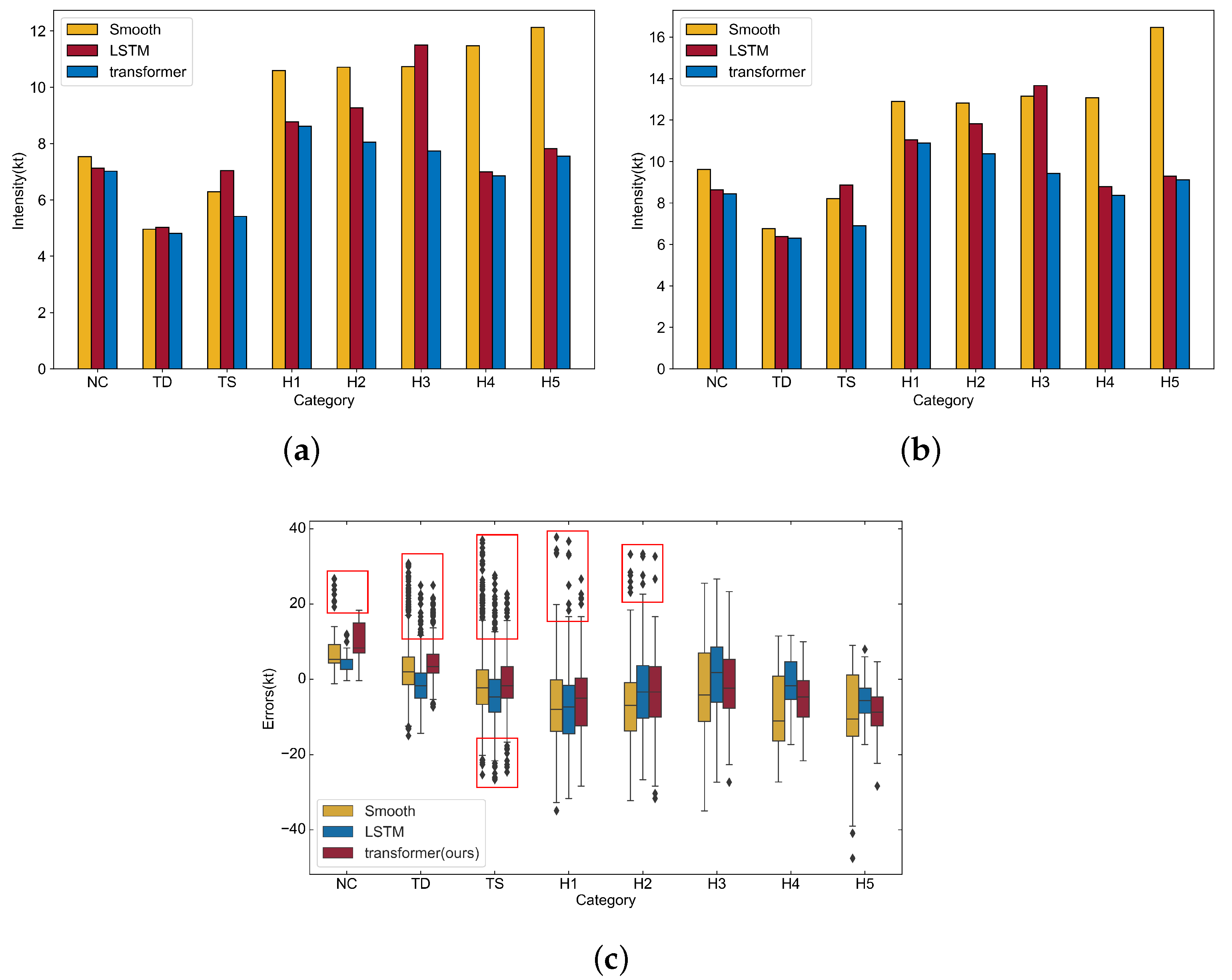
To demonstrate the effectiveness of our transformer, we compared it with LSTM and the smooth procedure. We set the length of the sequence to 7 in the transformer and LSTM. In the smooth procedure, we used a weighted average operation and the weights are 5, 4, 3, 2, and 1. The MAE and RMSE results on each category are shown in Figure 5. The transformer exhibited a better performance with both RMSE and MAE metrics in all categories than the other two methods. The box plots of these three methods are shown in Figure 5c. In Figure 5c, we use a red rectangle to mark some outliers and we can see that our transformer has fewer outliers than other methods. Additionally, our transformer has a smaller interquartile range, which means the estimation is more stable.
We further selected six representative typhoons during 2017 from five regions (Atlantic, West Pacific, East Pacific, Indian Ocean, and Southern Hemisphere). We present their estimations, predictions, and trends in detail. The 3-hourly intensity estimation comparison is shown in Figure 6. The maximum intensities of these six typhoons (Kenneth, Eugene, Cook, Talim, Gert, and Mora) are 115, 100, 90, 90, 95, and 80 knots, respectively.

5. Conclusions

In this paper, we proposed a DR-transformer framework to estimate and predict TC intensity. The framework is a three-step pipeline to fuse features of TC, consisting of (1) a DR-extractor to extract the individual feature of TC, (2) a transformer to aggregate the temporal feature, and (3) a classifier to reach the final result. Experimental results show that TC feature representation could largely benefit from distance-consistency and rotation-invariance feature learning. Additionally, we lead the way of using transformers to obtain a temporal correlation of images and prove its great potential. This framework is applied to the practical TC intensity estimation and can obtain TC intensity from its image in only 186 ms on a single CPU, which fully meets actual business needs.
In summary, our work has demonstrated a valuable method to solve the bottleneck in the field of tropical cyclone forecasting. We hope that this work will play a role in weather forecasting. In the future, our method, as a general feature extraction framework, can be extended to most of the numerical prediction studies in the meteorological field.

Author Contributions

Y.X. and Y.L. conceived and designed the research. Y.L. and S.L. designed and supervised the evaluation results. Q.Q. provided context for business applications. Y.L. wrote the original draft and Y.X., S.L., Q.Q. and B.X. helped to revise the manuscript. All authors have read and agreed to the published version of the manuscript.

Funding

This work was supported by the National Natural Science Foundation of China (NSFC No. 62076031).

Institutional Review Board Statement

Not applicable.

Informed Consent Statement

Not applicable.

Data Availability Statement

The processed data presented in this study are available on request from the corresponding author.

Acknowledgments

The authors would like to thank all the teachers and others that take part in this work.

Conflicts of Interest

The authors declare no conflict of interest.

Abbreviations

The following abbreviations are used in this manuscript:
TCTropical Cyclone
DCDistance Consitency
RIRotation Invariance
DRDistance consitency and Rotation invariance

References

  1. Dvorak, V.F. Tropical Cyclone Intensity Analysis and Forecasting from Satellite Imagery. Mon. Weather Rev. 1975, 103, 420–430. [Google Scholar] [CrossRef]
  2. Pradhan, R.; Aygun, R.S.; Maskey, M.; Ramachandran, R.; Cecil, D.J. Tropical Cyclone Intensity Estimation Using a Deep Convolutional Neural Network. IEEE Trans. Image Process. 2018, 27, 692–702. [Google Scholar] [CrossRef]
  3. Chen, B.; Chen, B.F.; Lin, H.T. Rotation-blended CNNs on a New Open Dataset for Tropical Cyclone Image-to-intensity Regression. In Proceedings of the 24th ACM SIGKDD International Conference, London, UK, 19–23 August 2018. [Google Scholar]
  4. Chen, B.; Chen, B.; Lin, H.T.; Elsberry, R.L. Estimating Tropical Cyclone Intensity by Satellite Imagery Utilizing Convolutional Neural Networks. Weather Forecast. 2019, 34, 447–465. [Google Scholar] [CrossRef]
  5. Vaswani, A.; Shazeer, N.; Parmar, N.; Uszkoreit, J.; Jones, L.; Gomez, A.N.; Kaiser, L.; Polosukhin, I. Attention Is All You Need. In Proceedings of the 31st Conference on Neural Information Processing Systems (NIPS 2017), Long Beach, CA, USA, 4–9 December 2017. [Google Scholar]
  6. Xu, Y.; Yang, H.; Cheng, M.; Li, S. Cyclone intensity estimate with context-aware cyclegan. In Proceedings of the 2019 IEEE International Conference on Image Processing (ICIP), Taipei, Taiwan, 22–25 September 2019; pp. 3417–3421. [Google Scholar]
  7. Chen, B.; Chen, B.F.; Chen, Y.N. Real-time Tropical Cyclone Intensity Estimation by Handling Temporally Heterogeneous Satellite Data. arXiv 2020, arXiv:2010.14977. [Google Scholar]
  8. Cover, T.; Hart, P. Nearest neighbor pattern classification. IEEE Trans. Inf. Theory 1967, 13, 21–27. [Google Scholar] [CrossRef]
  9. Bromley, J.; Bentz, J.; Bottou, L.; Guyon, I.; Lecun, Y.; Moore, C.; Sackinger, E.; Shah, R. Signature Verification using a “Siamese” Time Delay Neural Network. Int. J. Pattern Recognit. Artif. Intell. 1993, 7, 25. [Google Scholar] [CrossRef] [Green Version]
  10. Chopra, S.; Hadsell, R.; LeCun, Y. Learning a similarity metric discriminatively, with application to face verification. In Proceedings of the 2005 IEEE Computer Society Conference on Computer Vision and Pattern Recognition (CVPR’05), San Diego, CA, USA, 20–25 June 2005; Volume 1, pp. 539–546. [Google Scholar] [CrossRef]
  11. Hadsell, R.; Chopra, S.; Lecun, Y. Dimensionality Reduction by Learning an Invariant Mapping. In Proceedings of the 2006 IEEE Computer Society Conference on Computer Vision and Pattern Recognition (CVPR’06), New York, NY, USA, 17–22 June 2006. [Google Scholar]
  12. Hoffer, E.; Ailon, N. Deep Metric Learning Using Triplet Network. In Proceedings of the International Workshop on Similarity-based Pattern Recognition, Copenhagen, Denmark, 12–14 October 2015. [Google Scholar]
  13. Schroff, F.; Kalenichenko, D.; Philbin, J. FaceNet: A Unified Embedding for Face Recognition and Clustering. arXiv 2015, arXiv:1503.03832. [Google Scholar]
  14. Sohn, K. Improved Deep Metric Learning with Multi-Class N-Pair Loss Objective. In NIPS’16: Proceedings of the 30th International Conference on Neural Information Processing Systems; Curran Associates Inc.: Red Hook, NY, USA, 2016; pp. 1857–1865. [Google Scholar]
  15. Sun, Y.; Cheng, C.; Zhang, Y.; Zhang, C.; Zheng, L.; Wang, Z.; Wei, Y. Circle Loss: A Unified Perspective of Pair Similarity Optimization. arXiv 2020, arXiv:2002.10857. [Google Scholar]
  16. Kim, S.; Seo, M.; Laptev, I.; Cho, M.; Kwak, S. Deep Metric Learning Beyond Binary Supervision. In Proceedings of the IEEE/CVF Conference on Computer Vision and Pattern Recognition (CVPR), Long Beach, CA, USA, 16–20 June 2019. [Google Scholar]
  17. Devlin, J.; Chang, M.; Lee, K.; Toutanova, K. BERT: Pre-training of Deep Bidirectional Transformers for Language Understanding. arXiv 2018, arXiv:1810.04805. [Google Scholar]
  18. Brown, T.B.; Mann, B.; Ryder, N.; Subbiah, M.; Kaplan, J.; Dhariwal, P.; Neelakantan, A.; Shyam, P.; Sastry, G.; Askell, A.; et al. Language Models are Few-Shot Learners. arXiv 2020, arXiv:2005.14165. [Google Scholar]
  19. Raffel, C.; Shazeer, N.; Roberts, A.; Lee, K.; Narang, S.; Matena, M.; Zhou, Y.; Li, W.; Liu, P.J. Exploring the Limits of Transfer Learning with a Unified Text-to-Text Transformer. arXiv 2019, arXiv:1910.10683. [Google Scholar]
  20. Parmar, N.; Vaswani, A.; Uszkoreit, J.; Kaiser, L.; Shazeer, N.; Ku, A. Image Transformer. In Proceedings of the 35th International Conference on Machine Learning, Stockholm, Sweden, 10–15 July 2018. [Google Scholar]
  21. Dosovitskiy, A.; Beyer, L.; Kolesnikov, A.; Weissenborn, D.; Zhai, X.; Unterthiner, T.; Dehghani, M.; Minderer, M.; Heigold, G.; Gelly, S.; et al. An Image is Worth 16 × 16 Words: Transformers for Image Recognition at Scale. arXiv 2020, arXiv:2010.11929. [Google Scholar]
  22. Wu, B.; Xu, C.; Dai, X.; Wan, A.; Zhang, P.; Yan, Z.; Tomizuka, M.; Gonzalez, J.; Keutzer, K.; Vajda, P. Visual Transformers: Token-based Image Representation and Processing for Computer Vision. arXiv 2020, arXiv:2006.03677. [Google Scholar]
  23. Carion, N.; Massa, F.; Synnaeve, G.; Usunier, N.; Kirillov, A.; Zagoruyko, S. End-to-End Object Detection with Transformers. arXiv 2020, arXiv:2005.12872. [Google Scholar]
  24. He, K.; Zhang, X.; Ren, S.; Sun, J. Deep Residual Learning for Image Recognition. In Proceedings of the 2016 IEEE Conference on Computer Vision and Pattern Recognition (CVPR), Las Vegas, NV, USA, 26 June–1 July 2016; pp. 770–778. [Google Scholar] [CrossRef] [Green Version]
  25. Deng, J.; Dong, W.; Socher, R.; Li, L.-J.; Li, K.; Li, F. Imagenet: A large-scale hierarchical image database. In Proceedings of the 2009 IEEE Conference on Computer Vision and Pattern Recognition, Miami, FL, USA, 20–25 June 2009; pp. 248–255. [Google Scholar]
  26. Kingma, D.P.; Ba, J. Adam: A Method for Stochastic Optimization. arXiv 2017, arXiv:1412.6980. [Google Scholar]
  27. Liu, L.; Jiang, H.; He, P.; Chen, W.; Liu, X.; Gao, J.; Han, J. On the Variance of the Adaptive Learning Rate and Beyond. arXiv 2020, arXiv:1908.03265. [Google Scholar]
  28. Olander, T.; Velden, C. The Advanced Dvorak Technique (ADT) for Estimating Tropical Cyclone Intensity: Update and New Capabilities. Weather Forecast. 2019, 34, 905–922. [Google Scholar] [CrossRef]
  29. Kidder, S.; Goldberg, M.; Zehr, R.; Demaria, M.; Purdom, J.; Velden, C.; Grody, N.; Kusselson, S. Satellite Analysis of Tropical Cyclones Using the Advanced Microwave Sounding Unit (AMSU). Bull. Am. Meteorol. Soc. 2000, 81. [Google Scholar] [CrossRef] [Green Version]
  30. Herndon, D.; Velden, C. A Consensus Approach for Estimating Tropical Cyclone Intensity from Meteorological Satellites: SATCON. Weather Forecast. 2020, 35, 805–922. [Google Scholar]
  31. Fetanat, G.; Homaifar, A.; Knapp, K.R. Objective Tropical Cyclone Intensity Estimation Using Analogs of Spatial Features in Satellite Data. Weather Forecast. 2013, 28, 1446–1459. [Google Scholar] [CrossRef]
  32. Ritchie, E.A.; Wood, K.M.; Rodríguez-Herrera, O.G.; Pieros, M.F.; Tyo, J.S. Satellite-Derived Tropical Cyclone Intensity in the North Pacific Ocean Using the Deviation-Angle Variance Technique. Weather Forecast. 2014, 29, 505–516. [Google Scholar] [CrossRef] [Green Version]
  33. Liu, C.C.; Liu, C.Y.; Lin, T.H.; Chen, L.D. A satellite-derived typhoon intensity index using a deviation angle technique. Int. J. Remote Sens. 2015, 36, 1216–1234. [Google Scholar] [CrossRef]
  34. Zhao, Y.; Zhao, C.; Sun, R.; Wang, Z. A Multiple Linear Regression Model for Tropical Cyclone Intensity Estimation from Satellite Infrared Images. Atmosphere 2016, 7, 40. [Google Scholar] [CrossRef] [Green Version]
  35. Miller, J.; Maskey, M.; Berendes, T. Using Deep Learning for Tropical Cyclone Intensity Estimation. In Proceedings of the 2017 American Geophysical Union (AGU) Fall Meeting, New Orleans, LA, ISA, 11–15 December 2017; p. IN11E-05. [Google Scholar]
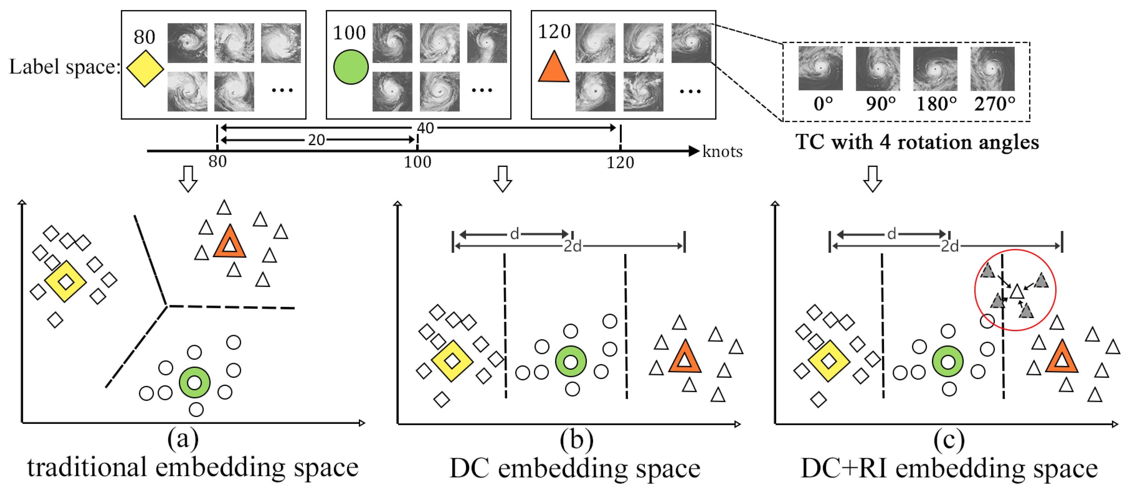
Figure 1. Comparison between typical method and ours. Compared with (a), the DC embedding space (b) is more consistent in terms of feature and distance. In the red circle of (c), RI embedding space can help the same tropical cyclone with different angles to reach a more accurate intensity.
Applsci 11 06208 g001
Figure 2. The overall pipeline of the proposed DR-transformer framework. During the inference stage, a series of the image is fed into the DR-extractor to generate the feature vectors sequentially. Meanwhile, we encode the intensity (estimated from classifier) to a one-hot vector. Then, the transformer takes one-hot vectors and feature vectors as input. Finally, the outputs of the transformer pass through a classifier to estimate and predict the intensity.
Applsci 11 06208 g002
Figure 3. Training details of DC loss. We construct a (N + 1)-tuplet of training samples with an anchor and N neighbors and feed them to DR-extractor. Finally, we calculated the DC loss of feature embeddings and intensities.
Applsci 11 06208 g003
Figure 4. From (ad) are the scatter of Npair, CE, log-ratio, and ours (DC + RI) respectively. The horizontal axis represents the groundtruth and the vertical axis represents predicted intensity. The blue line from bottom left to top right represents the best prediction. The grey, orange, and red crosses in the figure represent the errors within 10 knots, between 10 and 20 knots, and greater than 20 knots, respectively. In (c), the prediction distribution is very sparse due to the imbalance of categories.
Applsci 11 06208 g004
Figure 5. (a,b) are the comparison of MAE, RMSE respectively. And (c) is the box plot of estimated errors. The MAE and RMSE comparisons of the smooth procedure, LSTM, and transformer are shown in (a,b). The box plot of estimated errors of these three methods is shown in (c). In (c), we use a red rectangle to mark some outliers and we can see that our transformer has fewer outliers than other methods.
Applsci 11 06208 g005
Figure 6. Every 3-hour intensity estimation results of three methods (Smooth, LSTM, and transformer). We selected six representative typhoons during 2017 from five regions (East Pacific, Southern Hemisphere, West Pacific, Atlantic, and Indian Ocean). From (af) are Kenneth from East Pacific, Eugene from East Pacific, Cook from Southern Hemisphere, Talim from West Pacific, Gert from Atlantic, and Mora from Indian Ocean respectively.
Applsci 11 06208 g006
Table 1. Tropical cyclone estimation results compared with other methods. Bold numbers denote the best results. The second column represents the different ways we handled temporal data.
ApproachTemporalRmse (kt)
1FASI [31]-12.70
2Improved DAV-T [32]-12.70
3TI index [33]-9.34
4Y. Zhao (2016) [34]-12.01
5J. Miller (2017) [35]-10.00
6R. Pradhan (2018) [2]-10.18
7CNN-TC [3]-10.18
8Cross-entropy-10.36
9Npair [14]-10.75
10log-ratio [16]-10.21
11Ours (DC + RI)-8.88
12ADT [28]smooth11.79
13AMSU [29]smooth14.10
14SATCON [30]smooth9.21
15CNN-TC(S) [4]smooth8.39
16Ours (DR + smooth)smooth9.16
17Ours (DR + LSTM)LSTM8.67
18Ours (DR + transformer)transformer7.76
Table 2. Tropical cyclone estimation results compared with other methods. Bold numbers denote the best results. We divided tropical cyclones into eight categories by SSHWS based on their intensity and we counted the number of each category in the table. Additionally, we used MAE and RMSE as the evaluation metrics.
CategoryIntensity
Range
NumbersApproach
Cross-EntropyNpairLog-RatioOurs (DC + RI)
MAERMSEMAERMSEMAERMSEMAERMSE
H5≥137 kt419.0910.897.439.537.438.795.416.44
H4113–136 kt937.9610.1010.7913.327.449.416.829.26
H396–112 kt13012.2215.1815.1318.6311.9815.369.8712.35
H283–95 kt24311.9815.7113.6116.8210.8313.6610.3312.86
H164–82 kt46811.3514.0511.3414.1510.5613.0810.1912.40
TS34–63 kt17357.8410.018.1510.347.769.956.358.20
TD20–33 kt15015.017.445.507.256.788.435.437.03
NC<20 kt898.699.395.767.233.756.546.708.09
Total-43007.6310.368.0910.757.9010.216.798.88
Table 3. Ablation study on different components in DR-transformer framework. In the table, DC/RI/CE represents whether to use the corresponding loss and smooth/transformer represents the way we process temporal data.
LossMAERMSE
(a)CE7.6310.36
(b)DC7.449.71
(c)DC + RI6.798.88
(d)DC + RI + smooth6.879.16
(e)DC + RI + transformer6.067.76
Table 4. Estimation and prediction RMSE and MAE of our method. In our prediction experiment, the length of the input time series must be greater than the predicted length. Therefore, we put a ’-’ in any position to represent an unpredictable situation.
ApporachT = 3T = 4T = 5T = 6T = 7T = 8T = 9
MAERMSEMAERMSEMAERMSEMAERMSEMAERMSEMAERMSEMAERMSE
ours
(3 h-predict)
6.468.536.458.526.418.446.588.846.428.516.478.546.308.09
ours
(6 h-predict)
7.319.807.009.357.119.467.149.676.939.307.049.936.538.55
ours
(12 h-predict)
--9.2312.658.9212.418.5711.858.6611.917.6510.52
ours
(24 h-predict)
------12.1217.16
ours
(estimate)
6.137.966.087.826.117.917.928.046.017.766.167.936.798.67
Publisher’s Note: MDPI stays neutral with regard to jurisdictional claims in published maps and institutional affiliations.