Motion Planning for a Mobile Humanoid Manipulator Working in an Industrial Environment

Abstract

This paper presents the usage of holonomic mobile humanoid manipulators to carry out autonomous tasks in industrial environments, according to the smart factory concept and the Industry 4.0 philosophy. The problem of transporting lengthy objects, taking into account mechanical limitations, the conditions for avoiding collisions, as well as the dexterity of the manipulator arms was considered. The primary problem was divided into three phases, leading to three different types of robotic tasks. In the proposed approach, the pseudoinverse Jacobian method at the acceleration level to solve each of the tasks was used. The redundant degrees of freedom were used to satisfy secondary objectives such as robot kinetic energy, the maximization of the manipulability measure, and the fulfillment mechanical and collision-avoidance limitations. A computer example involving a mobile humanoid manipulator, operating in an industrial environment, illustrated the effectiveness of the proposed method.

1. Introduction

The history of industrial robotics dates back to the 1950s. At that time, the first designs of numerically controlled machine tools and programmable manipulators for industrial applications were created. At the beginning of the 1960s, the first mass-produced robots were used in production processes, and a few years later, the first automated production line was created. In subsequent years, the use of automation systems increased, leading to the third industrial revolution in the 1970s. This stage, in the development of robotics, was characterized by the use of relatively simple robots that performed repetitive tasks that had been planned in advance. The fourth industrial revolution, known as Industry 4.0, has now already begun, leading to smart factories and autonomous systems that complete production processes without human intervention [1,2]. Such developments require the use of sensors and new ideas to control algorithms, thus allowing operations to be carried out autonomously. According to the philosophy of Industry 4.0, manufacturing is required to be ever faster and more efficient, in order that companies might strive to increase the degree of automation [3]. Due to the necessity of meeting the needs of individual customers, interest in the application of knowledge transfer support [4,5] is growing.

At present, stationary manipulators predominate in many industrial applications. Their main advantages are their agility and manual dexterity and the ability to perform tasks with high precision. On the other hand, the working space for this type of robotic mechanism is limited by the length of the arm, which reduces the possibilities of their use. This results in an increased interest in mobile platforms [6], whose working space is only limited by the elements of the equipment present in their surroundings. Unfortunately, these type of robots are much less precise than stationary manipulators and usually do not have their manipulation abilities, so they are mainly used to solve simple logistic tasks, such as the transportation of pallets [7]. The combination of the advantages of both systems is a mobile manipulator, which consists of a mobile platform and a manipulator mounted on top. The use of this type of robotic system allows the working space to be enlarged and high precision, in the completion of tasks, to be maintained. Moreover, it allows several stationary manipulators to be replaced with one mobile manipulator moving between different workstations. A review of the main industrial domains suitable for such systems was presented in the works [8,9].

There are, however, some types of tasks that cannot be executed by a single robot. Such tasks are associated with the movement of heavy objects that a single robot cannot lift, due to the physical limitations of its actuators or, again, due to the movement of the large objects, which must be supported at several points. The necessity of solving such problems leads to the deployment of cooperating robots performing a common task. The method of the motion planning of multiple mobile manipulators moving a common rigid object was presented in [10]. As shown in practical applications, the use of cooperating robots results in additional problems related to the necessity for the coordination of the movement of mobile platforms. On the other hand, there are tasks, such as the handling of lengthy objects and peg-in-hole assemblies, etc., where the use of several, individual robots is unnecessary. It seems simply providing a grip at several points is quit sufficient, and in such cases, multi-arm systems, such as humanoid robots, can be used successfully. Moreover, mounting such a system onto a mobile platform increases the operating range significantly and simultaneously maintains the precision of manipulation. For this reason, both stationary and mobile humanoid manipulators have become the subject of growing interest in recent years. Typical solutions for the motion planning problems cannot be used directly for robots of this type, because in this case, it is necessary to take into account additional conditions such as closed-loop constraints, the manipulability of multiarm system, etc. There are several approaches to motion planning of humanoid robots. According to the review presented in [11], the most motion generation methods, due to the requirement of simplicity, are addressed using only kinematics. The method based on master–slave coordination such as the stationary, dual-arm, Baxter robot, working on an assembly line and completing peg-in-hole tasks, was presented in the work [12]. The use of highly redundant humanoid mobile manipulators was proposed in [13]. The authors designed the motion planning algorithms to carry out “human-like” autonomous navigation and manipulation tasks. The redundancy resolution scheme for humanoid manipulators, equipped with differential driven platforms, was presented in [14]. The validity of the algorithm was checked by simulating the robot, in tracing the global optimal path generated by the $A^{*}$ (A-star) graph search algorithm. It is worth noting that research on humanoid robotic systems is not just limited to industrial applications. Such systems are also utilized as support for disabled and elderly people [15], medical assistants [16], and service robots for intelligent or smart homes [17]. The solutions obtained in these areas can also be used in industrial applications.

The mobility of robotic systems can be realized in different ways. In the case of humanoid manipulators, the use of human-like bipedal platforms seems to be natural [18]. Unfortunately, such a solution causes many technical problems that have not been solved satisfactorily. Additionally, walking robots can be useful in difficult, natural conditions; however, in an industrial environment, the use of wheeled robots is more efficient because this allows higher velocity to be achieved in the robotic system. The choice of the drive type used is also important. Wheeled platforms can be divided into the holonomic type, which can move in any direction, since they have three degrees of freedom, and the nonholonomic type, which are systems whose movement is subject to the constraint of rolling without slipping. The motion planning methods for mobile robots presented above have concerned systems equipped with nonholonomic platforms, but it seems that in industrial conditions, the use of holonomic platforms is justified. Such systems, equipped with Mecanum-type wheels, for example, perform well on the even surface of a production or warehouse hall, and the lack of movement limitations makes it possible to move in a cluttered environment and significantly increases the usefulness of the robot.

In this paper, the trajectory planning method for a humanoid dual-arm manipulator mounted on a holonomic wheeled mobile platform, inspired by the Rollin’ Justin [19] robot, was considered. The main goal of this work was to present the general framework for the motion planning of such systems. In contrast to other solutions, presented in the literature, the comprehensive approach to the execution of the robot task in an industrial environment was proposed. Solving the problem of the handling of lengthy objects, while simultaneously gripping such objects at several points, is something of a priority and was taken into account. In this case, the task of the robot, in the general form, can be divided into three phases, viz., move-to-grip, where the robot moves towards the object, moving the object to a specified location, and precise manipulation along a prescribed path. The proposed approach allows the motion planning problem to be resolved in all three phases. Moreover, in the presented method, the series of constraints, resulting from the mechanical properties of the mechanism and the boundary constraints resulting from the task, was considered. The constraints imposed on the mechanical limits of joint angles, as well as the constraints connected with potential collisions among the robot, its environment, the object being handled, and the inner collisions between the robot arms were taken into account, in particular. Additionally, motions were planned in order to maximize the instantaneous manipulability measure, in order to avoid manipulator singularities during movement and to ensure the high dexterity of the robot at the end of each phase of a particular task. Such an approach allows the next phase to be performed without the necessity of reconfiguration. In order to solve the robot task, formulated in the above manner, the Jacobian pseudoinverse method at the acceleration level with secondary objective functions was used. The application of the Jacobian pseudoinverse matrix is a common approach [20,21,22] in resolving redundancy, due to its effectiveness and the possibility of being able to use computations in real time. The efficiency of the proposed algorithm was confirmed by computer simulation, involving a humanoid mobile robot, in its completion of three phases of the transportation of a lengthy object.

The paper is organized as follows. Section 2 presents the mathematical models, both of the robot and of the object (Section 2.1). The formulation of the robot task and constraints are taken into account (Section 2.2), as well as the solution for the three phases of the robot task (Section 2.3 and Section 2.4). The simulations performed are presented in Section 3, and their results are discussed in Section 4. A summary of the research undertaken and the future direction thereof is presented in Section 5.

2. Materials and Methods

2.1. Model of the System

In the paper, a holonomic mobile humanoid manipulator, working in an industrial environment, was considered. The robot was inspired by the Rollin’ Justin robot [19], developed by the German Aerospace Center (DLR), which is made up of a humanoid dual-arm upper body, mounted on a mobile platform. In contrast to the original design, the robot proposed in this work was equipped with a holonomic $(3,0)$-type platform with two pairs of Mecanum wheels and the arms with four DOF. The model of the humanoid manipulator on its holonomic platform is shown in Figure 1. As can be seen, the robot consists of four main components:

• The 3DOF holonomic platform, which allows any position and orientation to be achieved in the $XY$-plane of the workspace;
• The 3DOF torso with three revolute joints and an additional, passive revolute joint, placed at the end of the kinematic chain, ensuring that the chest is always kept orthogonally to the ground;
• Two arms, each with 4DOF.

In the work here presented, and for the sake of simplicity and in order to increase the readability of the presentation, the orientation of the end-effectors was not taken into account. Such an assumption does not affect the generality of the presented approach because the proposed method did not limit the number of arm joints, so it is possible to complement the arms with additional 3DOF grippers. The problem with planning a grasping action is beyond the scope of this work; however, it is the subject of ongoing research, and the results presented in such as [23] can be utilized when considering the humanoid manipulator in this paper.

It was assumed that the humanoid robot consisted of a series of rigid bodies connected by rigid joints. In this case, the location of each link with respect to a previous link can be easily described by the location, i.e., the position and orientation of the local coordinate frame, attached rigidly to the chosen link, relative to the local coordinate frame attached to the previous link. In order to describe the position of the two end-effectors, i.e., the left and right arms of the robot, in the workspace, modified Denavit–Hartenberg (DH) notation [24] was used, and the parameters of the robot joints and links were determined and are shown in

Table 1. DH parameters for the humanoid manipulator.

Torso					Left Arm					Right Arm
i	${\alpha }_{i-1}$	$a_{i-1}$	$d_i$	${\theta }_i$	i	${\alpha }_{i-1}$	$a_{i-1}$	$d_i$	${\theta }_i$	i	${\alpha }_{i-1}$	$a_{i-1}$	$d_i$	${\theta }_i$
1	$\pi /2$	0	$l_{T_1}$	$q_{T_1}$	1	$\pi$	0	$-l_{L_1}$	$q_{L_1}$	1	0	0	$l_{R_1}$	$q_{R_1}$
2	$\pi /2$	0	0	$q_{T_2}$	2	$\pi /2$	0	0	$q_{L_2}$	2	$-\pi /2$	0	0	$q_{R_2}$
3	0	$l_{T_2}$	0	$q_{T_3}$	3	$-\pi /2$	0	$-l_{L_2}$	$q_{L_3}$	3	$\pi /2$	0	$l_{R_2}$	$q_{R_3}$
4	0	$l_{T_3}$	0	$q_T^{*}$	4	$\pi /2$	0	0	$q_{L_4}$	4	$-\pi /2$	0	0	$q_{R_4}$

.

$l_{T_1},l_{T_2},l_{T_3},l_{L_1},l_{L_2},l_{R_1},l_{R_2}$ are the lengths of the humanoid links for the torso and the left and right arms, respectively. $q_{T_1},q_{T_2},q_{T_3}$ are the joints angles of the torso. $q_T^{*}=pi/2-q_{T_2}-q_{T_3}$ is the joint angle of the last joint of the torso and is used to compensate the rotations of the two previous joints. $q_{L_1}\cdots q_{L_4},q_{R_1}\cdots q_{R_4}$ are the joint angles of the left and right arms, respectively. The rotation axes of the independent joints of the torso (i.e., the axes for the first, second, and third joints) and all joint axes of left arm are shown in Figure 1; the rotation axes of the right arm are similar. As shown, the arms are located at the end of the torso, and their bases are rotated by an angle of $\beta$. The grippers are located at distances $l_{L_3}$ and $l_{R_3}$ from the fourth joints of the left and right arm, respectively.

The position and orientation of the holonomic platform is uniquely defined by three parameters: x and y determine the platform center location in the $XY$ plane, and $\theta$ describes the platform orientation. Finally, the configuration of the four main parts of the humanoid can be described by four vectors:

$$\begin{array}{cc}{\mathbf{q}}_P={\left[x,y,\theta \right]}^T,\hfill & {\mathbf{q}}_T={\left[q_{T_1},q_{T_2},q_{T_3}\right]}^T,\hfill \\ {\mathbf{q}}_L={\left[q_{L_1},q_{L_2},q_{L_3},q_{L_4}\right]}^T,\hfill & {\mathbf{q}}_R={\left[q_{R_1},q_{R_2},q_{R_3},q_{R_4}\right]}^T\hfill \end{array}$$

while the configuration of the whole robot is described by the n-element vector of the generalized coordinates (in this case, $n=14$).

$$\mathbf{q}={\left[{\mathbf{q}}_P^T,{\mathbf{q}}_T^T,{\mathbf{q}}_L^T,{\mathbf{q}}_R^T\right]}^T.$$

(1)

Using the coordinate vector (1) and the parameters of the robot collected in Table 1, it is possible to determine the kinematic model of the system $\mathbf{f}\left(\mathbf{q}\right)$, describing the positions of the end-effectors in the workspace, which can be written in compact form, as follows:

$$\mathbf{p}=\mathbf{f}\left(\mathbf{q}\right)=\left[\begin{array}{c}{\mathbf{f}}_L\left(\mathbf{q}\right)\\ {\mathbf{f}}_R\left(\mathbf{q}\right)\end{array}\right],$$

(2)

where $p\in {\mathbb{R}}^{2m}$ is the vector with the positions of the humanoid end-effectors expressed in the workspace global frame, m is the dimension of the robot task, and ${\mathbf{f}}_L\left(\mathbf{q}\right),{\mathbf{f}}_R\left(\mathbf{q}\right)$ are the functions describing the positions of the left and right end-effectors.

The linear velocities of the end-effectors are given by differential kinematics as:

$$\dot{\mathbf{p}}=\mathbf{J}\left(\mathbf{q}\right)\dot{\mathbf{q}},$$

(3)

where $\dot{\mathbf{p}}$ is the vector containing the linear velocities of the end-effectors, $\dot{\mathbf{q}}$ is the vector of the generalized velocities of the robot joints, and $\mathbf{J}=\partial \mathbf{f}\left(\mathbf{q}\right)/\partial \mathbf{q}$ is the $(2m\times n)$-dimensional Jacobian matrix of the humanoid manipulator, which can be written as:

$$\mathbf{J}\left(\mathbf{q}\right)=\left[\begin{array}{ccc}{\mathbf{J}}_{L,torso}& {\mathbf{J}}_{L,larm}& 0\\ {\mathbf{J}}_{R,torso}& 0& {\mathbf{J}}_{R,rarm}\end{array}\right],$$

(4)

where ${\mathbf{J}}_{L,torso}=\partial {\mathbf{f}}_L\left(\mathbf{q}\right)/\partial {\mathbf{q}}_T$, ${\mathbf{J}}_{L,larm}=\partial {\mathbf{f}}_L\left(\mathbf{q}\right)/\partial {\mathbf{q}}_L$, ${\mathbf{J}}_{R,torso}=\partial {\mathbf{f}}_R\left(\mathbf{q}\right)/\partial {\mathbf{q}}_T$, ${\mathbf{J}}_{R,rarm}=\partial {\mathbf{f}}_R\left(\mathbf{q}\right)/\partial {\mathbf{q}}_R$.

Considering the transportation task, it is necessary to take into account the model of the object transported by the robot. In this work, it was assumed that the object was rigid and connected to the end-effectors of the robot. In this case, the location of the object in the workspace can be described by the 6-element vector $\mathbf{o}$:

$$\mathbf{o}={\left[{\chi }^T,{\varphi }^T\right]}^T,$$

(5)

where $\chi$ and $\varphi$ are the 3-element vectors describing the position and orientation of the local frame in the workspace global frame. The method does not limit the choice of the origin of the object coordinate frame, so it can be attached to the object at any given point.

2.2. Formulation of the Problem

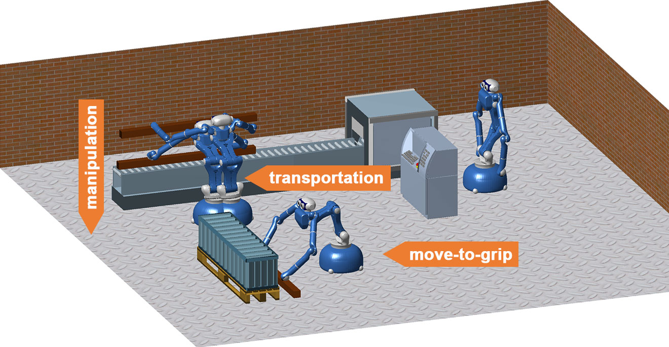
From the perspective of Industry 4.0, the use of information from the integral sensors of the robot, as well as from the sensors located in its surroundings allows tasks that, formerly, had to be planned in detail to now be completed autonomously. The basic idea of a task-motion-planning system for the task of autonomous robot considered in this work is presented in Figure 2. Such a system consists of the Task Planner, which specifies the main goals for the robot based on information from the sensors, and the Motion Planner, which plans the robot motion, according to the goals from the Task Planner. Trajectories generated by the Motion Planner are transmitted to the Robotic System. In the presented work, it was assumed that the information from the Task Planner was known and only the subsequent phases of the transportation problem of the lengthy object, as represented by blue boxes in the diagram, remained to be considered.

According to the idea of the Motion Planner, presented in Figure 2, the considered task of a humanoid mobile manipulator transporting an object in an industrial environment is divided into three phases (subtasks), solved separately:

• Moving the end-effectors to the given location ${\mathbf{p}}_f$ starting from the current configuration ${\mathbf{q}}_0$ in order to approach the object to be moved;
• Moving the object to the specified location ${\mathbf{o}}_f$ in the workspace;
• Moving the object along a prescribed path $\phi \left(s\right)$ in order to complete a precise operation, such as an assembly task.

The first task was to move the end-effectors of the humanoid manipulator to the grip points specified by the Task Planner. This is a common, point-to-point task, in this case, to be undertaken by two end-effectors simultaneously. It can be expressed as:

$$\mathbf{f}\left(\mathbf{q}\left(T\right)\right)=\left[\begin{array}{c}{\mathbf{f}}_L\left(\mathbf{q}\left(T\right)\right)\\ {\mathbf{f}}_R\left(\mathbf{q}\left(T\right)\right)\end{array}\right]=\left[\begin{array}{c}{\mathbf{p}}_{L,f}\\ {\mathbf{p}}_{R,f}\end{array}\right]={\mathbf{p}}_f,$$

(6)

where T is the final moment of the motion and $p_f$ is the $2m$-element vector containing the final position of the left ${\mathbf{p}}_{L,f}$ and the right ${\mathbf{p}}_{R,f}$ end-effectors of the robot.

In the second and third task, it is necessary to take into account the object being transported by the robot. In the presented work, such tasks were formulated as the movement of the object in the workspace, where the motion of the robot was forced by the set of constraints resulting from the closed kinematic chain established by the robot arms and the object being held by them. In both cases, the robot began the movement from the initial configuration ${\mathbf{q}}_0$ holding the object; however, in the second task, achieving the desired final location was the only goal of any importance, while in the third task, the movement of the object was determined by the prescribed path $\phi \left(s\right)$.

In the second task, starting from the configuration achieved in the first one, the robot moved the object being transported to the position specified by the Task Planner. According to the above considerations, this task can be described as:

$$\mathbf{o}\left(T\right)={\mathbf{o}}_f.$$

(7)

Finally, the humanoid manipulator started from the final configuration of the previous task and carried out the precise manipulation of the object, according to the path determined by the Task Planner. Such a task can be written as follows:

$$\mathbf{o}\left(t\right)-\phi \left(s\right)=\mathbf{0},$$

(8)

where s is the scaling parameter, which depends on time t, i.e., $s=s\left(t\right)$, $s\in \left[0,1\right]$.

In both of the above cases, additional constraints resulting from grasping should be considered. The humanoid manipulator held the object at two contact points, and the hard finger model [25] of contact was assumed in this paper. This assumption means that the linear components of the velocities were transmitted through the contact point, while, on the other hand, the angular components were not. Introducing the function ${\mathbf{p}}_C\left(\mathbf{o}\right)$, describing the locations of the contact points, the grasp limitations can be expressed as geometric and kinematic constraints as follows:

$$\begin{array}{cc}\hfill \mathbf{f}\left(\mathbf{q}\right(t\left)\right)& ={\mathbf{p}}_C\left(\mathbf{o}\left(t\right)\right)\hfill \\ \hfill \mathbf{J}\dot{\mathbf{q}}\left(t\right)& ={\dot{\mathbf{p}}}_C\left(\mathbf{o}\left(t\right)\right),\hfill \end{array}$$

(9)

where ${\dot{\mathbf{p}}}_C=d{\mathbf{p}}_C/dt$ describes the linear velocities of the contact points.

The practical processes that are accomplished by the industrial robots impose some conditions at the beginning and the end of the trajectory. It is natural to assume that at the initial and final moments of the performance of the task, the velocities of the manipulator equal zero:

$$\dot{\mathbf{q}}\left(\mathbf{0}\right)=\mathbf{0},\dot{\mathbf{q}}\left(\mathbf{T}\right)=\mathbf{0}.$$

(10)

During the completion of the task, the robot should maintain the limitations resulting from its construction and the range of movements permitted in the individual joints. Introducing the scalar function $C_M$, defining the algebraic distance of a given configuration from the range permitted, such mechanical constraints can be expressed in the form of a set of $L_M$ inequalities in the form:

$$\forall t\in \left[0,T\right]C_M^i\left(\mathbf{q}\left(t\right)\right)\ge 0,i=1,\cdots ,L_M.$$

(11)

The space in which the robot operates may contain some equipment that should be treated as obstacles and must be taken into account during the motion planning. Introducing the scalar functions $C_{Or}$ and $C_{Oo}$, which describe the algebraic distances from the obstacles to the robot and object, respectively, the collision avoidance conditions can be written as sets of $L_{Or}$ for the robot and $L_{Oo}$ for the object inequalities in the form:

$$\forall t\in \left[0,T\right]C_{Or}^i\left(\mathbf{q}\left(t\right)\right)\ge 0,i=1,\cdots ,L_{Or}$$

(12)

$$\forall t\in \left[0,T\right]C_{Oo}^i\left(\mathbf{o}\left(t\right)\right)\ge 0,i=1,\cdots ,L_{Oo}$$

(13)

In practice, the configuration of the manipulator joints should be far away from singular configurations. In order to achieve this goal, the Yoshikawa manipulability measure [26], which describes the distance to singular configurations, may be maximized. The Yoshikawa manipulability index $\mu \left(\mathbf{q}\right)$ is proportional to the volume of the velocity ellipsoid. The semi-axes of this ellipsoid coincide with the eigenvectors of the matrix $\mathbf{J}{\mathbf{J}}^T$, the lengths of these semi-axes being equal to the square roots of the eigenvalues of $\mathbf{J}{\mathbf{J}}^T$. Since the product of the lengths of the semi-axes is proportional to the volume of the ellipsoid and the product of the eigenvalues of the matrix is equal to the determinant of the matrix, the manipulability measure may be calculated as: $\mu \left(\mathbf{q}\right)=\sqrt{det\left(\mathbf{J}{\mathbf{J}}^T\right)}$. It seems that in the case of a dual-arm humanoid manipulator, the avoidance of singular configurations of the robot arms [27] is important, so the following manipulability measure was taken into account:

$$\mu \left(\mathbf{q}\right)=\sqrt{det\left({\mathbf{J}}_{arms}{\mathbf{J}}_{arms}^T\right)},$$

(14)

where ${\mathbf{J}}_{arms}=\left[\begin{array}{cc}{\mathbf{J}}_{L,larm}& 0\\ 0& {\mathbf{J}}_{R,rarm}\end{array}\right]$ consists of the 8 last columns of the matrix (4).

2.3. Solution: Primary Tasks

According to the analysis from the previous section, the transportation task, considered in this work, consisted of three steps: moving the robot to the object, moving the object to a specific location, and moving the object along a prescribed path. The first step is a point-to-point task described by the dependency (6). In the presented approach, in order to eliminate, known from the literature, the drift effect resulting in a trajectory error increasing in time, a feedback loop algorithm, correcting the robot movement on the basis of the information from the sensors, was proposed. For this purpose, the following end-effector error function $\mathbf{e}\left(t\right)$ between the current and fixed final end-effectors positions was introduced:

$$\mathbf{e}\left(t\right)=\mathbf{f}\left(\mathbf{q}\right)-{\mathbf{p}}_f.$$

(15)

Using this function, the task of the robot can be presented in a more general form as:

$$\begin{array}{c}\hfill \underset{t\to \infty }{lim}\mathbf{e}\left(t\right)=\mathbf{0},\underset{t\to \infty }{lim}\dot{\mathbf{e}}\left(t\right)=\mathbf{0}.\end{array}$$

(16)

Such a formulation of the task allows reaching the final positions of the end-effectors, in a finite time, with any accuracy defined by the needs of the realized process. Moreover, in the proposed solution, the convergence rate and resulting final time were dependent on the gain coefficients and these can be tuned by their appropriate selection.

In order to solve the trajectory planning problem of the humanoid manipulator, the following system of differential equations was introduced:

$$\ddot{\mathbf{e}}(\mathbf{q},\dot{\mathbf{q}},\ddot{\mathbf{q}})+{\mathbf{K}}_d\dot{\mathbf{e}}(\mathbf{q},\dot{\mathbf{q}})+{\mathbf{K}}_p\mathbf{e}\left(\mathbf{q}\right)=\mathbf{0},$$

(17)

where ${\mathbf{K}}_d=\mathrm{diag}(K_d^1,\cdots ,K_d^{2m})$ and ${\mathbf{K}}_p=\mathrm{diag}(K_p^1,\cdots ,K_p^{2m})$ are $(2m\times 2m)$ diagonal gain matrices with positive coefficients, which determine the convergence rate of the solution of Equation (17).

The system (17) is a homogeneous differential equation with constant coefficients. In order to find the solution, $4m$ consistent dependencies should be given. They can be determined from the error function (15) for $t=0$, taking into account the initial condition (10). Moreover, using the Lyapunov stability theory and an approach similar to that presented in [28] for nonholonomic mobile manipulators, it is possible to show that the system is asymptotically stable, so the end-effector error $\mathbf{e}\left(t\right)$ and its derivative $\dot{\mathbf{e}}\left(t\right)$ converge to zero, guaranteeing fulfillment of the conditions (16). The convergence rate depends on the gain coefficients of matrices ${\mathbf{K}}_d$ and ${\mathbf{K}}_p$.

Determining the components $\ddot{\mathbf{e}}(\mathbf{q},\dot{\mathbf{q}},\ddot{\mathbf{q}})$, $\dot{\mathbf{e}}(\mathbf{q},\dot{\mathbf{q}})$ as:

$$\begin{array}{cc}\hfill \ddot{\mathbf{e}}(\mathbf{q},\dot{\mathbf{q}},\ddot{\mathbf{q}})& =\dot{\mathbf{J}}\left(\mathbf{q}\right)\dot{\mathbf{q}}+\mathbf{J}\left(\mathbf{q}\right)\ddot{\mathbf{q}},\hfill \\ \hfill \dot{\mathbf{e}}(\mathbf{q},\dot{\mathbf{q}})& =\mathbf{J}\left(\mathbf{q}\right)\dot{\mathbf{q}}\hfill \end{array}$$

(18)

and substituting them into System (17), the dependency that allows determining the trajectory of the humanoid can be written as:

$$\mathbf{J}\left(\mathbf{q}\right)\ddot{\mathbf{q}}+\mathbf{\upsilon }(\mathbf{q},\dot{\mathbf{q}})=\mathbf{0},$$

(19)

where $\mathbf{\upsilon }(\mathbf{q},\dot{\mathbf{q}})=\dot{\mathbf{J}}\left(\mathbf{q}\right)\dot{\mathbf{q}}+{\mathbf{K}}_d\mathbf{J}\left(\mathbf{q}\right)\dot{\mathbf{q}}+{\mathbf{K}}_p(\mathbf{f}\left(\mathbf{q}\right)-{\mathbf{p}}_f)$.

The dependency (19) formulates the primary task of the humanoid manipulator, which grasps the object in the locations specified by vector ${\mathbf{p}}_f$. Due to the high redundancy of the humanoid $(n>2m)$, the Jacobian matrix $\mathbf{J}\left(\mathbf{q}\right)$ is rectangular (the number of its columns is greater than the number of its rows), and there is an infinite number of trajectories satisfying the condition (19). In order to find solution $\ddot{\mathbf{q}}$, the task can be formulated as a quadratic optimization problem with linear constraints, which leads to the determination of a trajectory minimizing a certain cost. Using the Moore–Penrose pseudoinverse of matrix $\mathbf{J}\left(\mathbf{q}\right)$, ${\mathbf{J}}^{†}\left(\mathbf{q}\right)={\mathbf{J}}^T{\left(\mathbf{J}{\mathbf{J}}^T\right)}^{-1}$, the optimal solution minimizing the acceleration norm of a mobile robot $\parallel \ddot{\mathbf{q}}\parallel$ and satisfying the linear constraints (19) can be determined as:

$$\ddot{\mathbf{q}}\left(t\right)=-{\mathbf{J}}^{†}\left(\mathbf{q}\right)\mathbf{\upsilon }(\mathbf{q},\dot{\mathbf{q}}).$$

(20)

The dependency (20) describes the trajectory realizing the primary task of a humanoid robot. The additional constraints imposed on the robot motion, as presented in the previous section, will be introduced as secondary objectives in the next section.

In the second step of the transportation task, the robot moves the object to the desired location ${\mathbf{o}}_f$. In order to solve this task, in the presented work, the method of trajectory planning for the object, guaranteeing fulfilling the dependency (7), while simultaneously determining suitable robot movement, was proposed. In this case, the object was considered as the single 6DOF joint, which can achieve any position and orientation in a 3-dimensional workspace, and its movement was planned using an idea similar to that used in a previous task. For this purpose, the following function $ϵ\left(t\right)$ describing the error between the current and desired fixed location of the object was introduced:

$$ϵ\left(t\right)=\mathbf{o}\left(t\right)-{\mathbf{o}}_f$$

(21)

and this task can be formulated as:

$$\begin{array}{c}\hfill \underset{t\to \infty }{lim}ϵ\left(t\right)=\mathbf{0},\underset{t\to \infty }{lim}\dot{ϵ}\left(t\right)=\mathbf{0}.\end{array}$$

(22)

Similarly, as in the case of the trajectory planning in the move-to-grip phase (22), such a formulation of the object task would allow achieving the desired location of the transported object with any accuracy in finite time.

Introducing the $(6\times 6)$ diagonal matrices with positive coefficients ${\mathcal{K}}_d$ and ${\mathcal{K}}_p$, the trajectory of the object can be determined from the following equation:

$$\ddot{ϵ}(\mathbf{o},\dot{\mathbf{o}},\ddot{\mathbf{o}})+{\mathcal{K}}_d\dot{ϵ}(\mathbf{o},\dot{\mathbf{o}})+{\mathcal{K}}_pϵ\left(\mathbf{o}\right)=\mathbf{0}$$

(23)

with respect to the initial conditions determined from (21) for $t=0$ and zero initial velocity of the object resulting from the lower condition (9) and (10). The stability of Equation (23) is assured by the assumed form of the gain matrices, guaranteeing the fulfillment conditions (22). Finally, similar to the previous task, after determining $\ddot{ϵ}(\mathbf{o},\dot{\mathbf{o}},\ddot{\mathbf{o}})$, $\dot{ϵ}(\mathbf{o},\dot{\mathbf{o}})$ and using the simple algebra, the trajectory of the object can be written as:

$$\ddot{\mathbf{o}}\left(t\right)=-{\mathcal{K}}_d\dot{\mathbf{o}}-{\mathcal{K}}_p(\mathbf{o}-{\mathbf{o}}_f).$$

(24)

Taking into account that the transported object is rigid and that the location of the grip points in the object frame is known (this was determined by the Task Planner), the location of the grip points in each time instant can be calculated using function ${\mathbf{p}}_C\left(\mathbf{o}\right)$. According to the proposed approach, the trajectory of the contact points, determined in this way, defines the trajectory tracking task to be performed by the robot in this phase.

In order to ensure suitable robotic movement, enabling the desired location of the object determined from (24) to be reached, the grasp limitations (9) must be satisfied, so the primary task of the robot, after introducing end-effector error $\mathbf{e}\left(t\right)$:

$$\mathbf{e}\left(t\right)=\mathbf{f}\left(\mathbf{q}\right)-{\mathbf{p}}_C\left(\mathbf{o}\left(t\right)\right),$$

(25)

may be formulated as:

$$\begin{array}{c}\hfill \underset{t\to \infty }{lim}\mathbf{e}\left(t\right)=\mathbf{0},\underset{t\to \infty }{lim}\dot{\mathbf{e}}\left(t\right)=\mathbf{0}.\end{array}$$

(26)

The trajectory of the robot, as in the case of the point-to-point task, can be determined from differential Equation (17) for a new form of error function introduced by the dependency (25) as follows:

$$\ddot{\mathbf{q}}=-{\mathbf{J}}^{†}\left(\mathbf{q}\right)\mathbf{\upsilon }(\mathbf{q},\dot{\mathbf{q}}).$$

(27)

where $\mathbf{\upsilon }(\mathbf{q},\dot{\mathbf{q}})=\dot{\mathbf{J}}\left(\mathbf{q}\right)\dot{\mathbf{q}}+{\mathbf{K}}_d(\mathbf{J}\left(\mathbf{q}\right)\dot{\mathbf{q}}-{\dot{\mathbf{p}}}_C)+{\mathbf{K}}_p(\mathbf{f}\left(\mathbf{q}\right)-{\mathbf{p}}_C)-{\ddot{\mathbf{p}}}_C$.

Due to the asymptotic stability of the differential Equation (17) and assuming that the initial condition (10) and the grasp limitations (9) at the initial moment of the motion are fulfilled (the robot is motionless and holds the object at contact points ${\mathbf{p}}_C$, so $\mathbf{e}\left(0\right)=0$ and $\dot{\mathbf{e}}\left(0\right)=0$), the error function $\mathbf{e}\left(t\right)=0$ and $\dot{\mathbf{e}}\left(t\right)=0$ at each instant, which guarantees the fulfillment of the grasp limitations while the robot is moving.

The task realized in the third step is similar to the second one, but the position and orientation of the object during the whole movement is given by the path $\varphi \left(s\right)$, preplanned earlier by the Task Planner, as shown in Figure 2. It was assumed that the path was given in parametric form as a function of scaling parameter s, dependent on time. In this case, the error function describing the distance between the current location of the object and the location determined by the path, extended by an additional element responsible for tracing the entire path, was introduced as follows:

$$\psi \left(t\right)=\left[\begin{array}{c}ϵ\left(t\right)\\ \xi \left(t\right)\end{array}\right]=\left[\begin{array}{c}\mathbf{o}\left(t\right)-\varphi \left(s\right)\\ s\left(t\right)-1\end{array}\right].$$

(28)

Using this function, the third task (8) can be described in a more general form as:

$$\begin{array}{c}\hfill \underset{t\to \infty }{lim}\psi \left(t\right)=\mathbf{0},\underset{t\to \infty }{lim}\dot{\psi }\left(t\right)=\mathbf{0}.\end{array}$$

(29)

Similarly, as in the first and second phase of the transportation task, such a formulation of the path tracking problem will allow achieving the final location of the object path with any accuracy. Moreover, if the object is not positioned precisely at the beginning of the path, the tracking error $\psi \left(t\right)$ will converge to zero during the object movement. Finally, the object trajectory and the path parameterization can be determined using the following system of differential equations:

$$\begin{array}{cc}\hfill \ddot{ϵ}(\mathbf{o},\dot{\mathbf{o}},\ddot{\mathbf{o}},s,\dot{s},\ddot{s})+{\mathcal{K}}_d\dot{ϵ}(\mathbf{o},\dot{\mathbf{o}},s,\dot{s})+{\mathcal{K}}_pϵ(\mathbf{o},s)& =\mathbf{0}\hfill \\ \hfill \ddot{\xi }\left(\ddot{s}\right)+{\kappa }_d\dot{\xi }\left(\dot{s}\right)+{\kappa }_p\xi \left(s\right)& =0.\hfill \end{array}$$

(30)

where the gain matrices ${\mathcal{K}}_d$ and ${\mathcal{K}}_p$ were accepted in the same way as in the second task and ensure the asymptotic stability of the first equation, and ${\kappa }_d$ and ${\kappa }_p$ are the positive scalars, which provide the asymptotic stability of the second equation. The property of the stability of Equation (30) implies the fulfillment of the conditions (29); moreover, if in the initial moment of motion, $\psi \left(0\right)=0$ and $\dot{\psi }\left(0\right)=0$ (the object is located at the beginning of the path, and $s\left(0\right)=0$), the object will be moved along the path for the whole process.

Finally, after simple calculations, the trajectory of the object $\mathbf{o}\left(t\right)$ and the path parameterization $s\left(t\right)$ can be determined from (30), in a manner similar to the previous tasks, using the initial conditions obtained from (28) for $t=0$ as follows:

$$\begin{array}{cc}\hfill \ddot{\mathbf{o}}\left(t\right)& =-{\mathcal{K}}_d\dot{\mathbf{o}}-{\mathcal{K}}_p(\mathbf{o}-\varphi \left(s\right))\hfill \\ \hfill \ddot{s}\left(t\right)& =-{\kappa }_d\dot{s}-{\kappa }_p(s-1).\hfill \end{array}$$

(31)

The manner for establishing the trajectory of the humanoid manipulator is the same as for the second task, so the trajectory of the robot is given by the dependency (27). Additionally, let us note that a similar approach, i.e., the motion along the given path, can be used to plan the grip of the object at the end of the move-to-grip phase.

2.4. Solution: Secondary Tasks

Due to its structure, the mobile humanoid manipulator has a high degree of redundancy, i.e., it has more degrees of freedom than are needed to perform the considered tasks. The existence of additional degrees of freedom makes it possible to introduce additional criteria that allow the manner in which the humanoid manipulator carries out the task to be determined. In such a case, a conflict between the primary task and additional limitations is possible. The problem can be solved by prioritizing individual tasks that will allow secondary goals to be achieved only if they do not violate the primary task. In a typical approach, the robot task was treated as the primary objective function, and additional conditions were included as secondary functions.

The tasks of the robot and the requirements determining how they are carried out are defined by the constraints introduced in the problem formulation section. The constraints imposed on the end-effector movement (6)–(9) specify the primary tasks of the robot and were taken into account along with the initial condition (10) in the solution presented in the previous section. The remaining limitations must be considered as secondary objectives of the tasks. In particular, as was shown in [29], the zero velocity of the end-effectors in the destination location, assured by the solution of the primary task, does not guarantee that the robot motion will come to a stop, once the task has been accomplished, thus satisfying the condition (10). In the case of the Jacobian pseudoinverse methods, it is important to provide the high manipulability measure of the robot (14) to avoid the loss of the Jacobian matrix rank. Moreover, the high manipulability in the destination location makes it easier to complete the next task. Finally, in practical applications, it is essential to fulfill the constraints resulting from the mechanical properties of the robot (11), as well as to avoid collisions during the robot motion in an industrial environment (12).

In order to fulfill the secondary objectives of the task, the following dependency, resulting from the ${\mathbf{J}}^{†}\left(\mathbf{q}\right)$ properties $\mathbf{J}{\mathbf{J}}^{†}=\mathbf{I}$, where $\mathbf{I}$ is the identity matrix, was used. The right multiplication of this dependency by $\mathbf{J}\left(\mathbf{q}\right)$ gives:

$$\mathbf{J}(\mathbf{I}-\mathbf{J}{\mathbf{J}}^{†})=\mathbf{0},$$

where $\mathbf{P}=\mathbf{I}-\mathbf{J}{\mathbf{J}}^{†}$ is the projection matrix on the null space of ${\mathbf{J}}^{†}\left(\mathbf{q}\right)$, and as a result, if ${\ddot{\mathbf{q}}}^{*}$ is a solution of the primary task of the robot, then for any chosen vector $\mathbf{v}$, the solution of this task is also a vector:

$$\ddot{\mathbf{q}}={\ddot{\mathbf{q}}}^{*}+\mathbf{P}\mathbf{v}.$$

(32)

Finally, it may be concluded that vector $\mathbf{v}$, projected by operator $\mathbf{P}$, allows the configuration of the robot to be changed without changing the positions of its end-effectors, so it may be used to satisfy the secondary objectives of the task [30]. This approach leads to a solution of the mobile robot in the following form:

$$\ddot{\mathbf{q}}=-{\mathbf{J}}^{†}\left(\mathbf{q}\right)\mathbf{\upsilon }(\mathbf{q},\dot{\mathbf{q}})+\mathbf{P}\mathbf{v}.$$

(33)

By choosing vector $\mathbf{v}$ in such a way as to optimize some additional criterion, it is possible to take into account a secondary objective in the form $H(\mathbf{q},\dot{\mathbf{q}})$. According to [30], mapping $H(\mathbf{q},\dot{\mathbf{q}})$ is usually taken as a mixed objective function:

$$H(\mathbf{q},\dot{\mathbf{q}})=\frac{1}{2}{\dot{\mathbf{q}}}^T\dot{\mathbf{q}}+H^{\prime }\left(\mathbf{q}\right),$$

(34)

whose minimization leads to a reduction in the velocities of the mobile robot and the fulfillment of the additional criteria described by mapping $H^{\prime }\left(\mathbf{q}\right)$. In this work, this additional term was used to maximize the manipulability measure and to satisfy the collision and mechanical constraints. For this purpose, function $H^{\prime }\left(\mathbf{q}\right)$ was taken as:

$$H^{\prime }\left(\mathbf{q}\right)=-\mu \left(\mathbf{q}\right)+D_{Or}\left(\mathbf{q}\right)+D_M\left(\mathbf{q}\right),$$

(35)

where $\mu (·)$ is the manipulability measure given by the dependency (14), $D_{Or}(·)$ denotes any continuous and differentiable internal penalty function, which increases when the robot approaches the obstacle surface, thus allowing the inequality constraints (12) to be fulfilled, and $D_M(·)$ is any continuous and differentiable function, which leads to the maximization of the distance of the configuration variables from the limits of the allowed range, resulting from the inequality constraints (11).

In order to find a solution of the robot task minimizing the criterion (34) and (35), the approach presented in [30], based on the steepest descent method, may be used, and vector $\mathbf{v}$ can be written in the following form:

$$\mathbf{v}=-\frac{\partial H}{\partial \mathbf{q}}-{\rho }_V\frac{\partial H}{\partial \dot{\mathbf{q}}},$$

(36)

where ${\rho }_V$ is a positive defined scalar describing the influence of the second term.

The approach presented above can be used for all types of humanoid manipulator tasks, supplementing the solutions (20) and (27) according to the dependency (33). It is worth noting that the proposed solution is pure kinematic at the acceleration level and does not take into account the dynamic properties of the robot. However, such an approach does not preclude practical applications of this method. Considering the physical capabilities of the robot actuators and the mass of the transported object, it is possible to determine suitable mechanical limitations that allow a real robot to perform the task. Moreover, the advantage of the kinematic approach is the lower computational burden of the algorithm.

In the case of the second task, planning the trajectory of the object was additionally required. The collision-free movement of the robot does not guarantee the collision-free movement of the object, so the object trajectory (24) must also take into account the conditions for avoiding collisions. The transported object did not have redundant degrees of freedom, so in this case, the avoidance of collisions cannot be performed using the secondary objective functions’ approach. On the other hand, in the second task, the final location was specified only, and the object can make any movement during the task execution. This makes it possible to take into account the conditions for avoiding collisions and supplementing the trajectory of the object (24) by the perturbation of the object accelerations in the neighborhoods of the obstacles. Finally, the trajectory of the object was proposed as:

$$\ddot{\mathbf{o}}\left(t\right)=-{\mathcal{K}}_d\dot{\mathbf{o}}-{\mathcal{K}}_p(\mathbf{o}-{\mathbf{o}}_f)-\frac{\partial D_{Oo}\left(\mathbf{o}\right)}{\partial \mathbf{o}},$$

(37)

where $D_{Oo}(·)$, as with the avoidance of collisions of the robot, denotes any continuous and differentiable internal penalty function, which takes the value 0 when the object is outside the zone surrounding the obstacle and increases when it approaches its surface, allowing the inequality constraints (13) to be fulfilled.

Let us note that in the third task, the object moved along the path preplanned by the Task Planner and did not collide with any obstacle in the workspace by definition, so the trajectory (31) did not require any modification.

3. Results

In order to verify the effectiveness of the proposed algorithm, computer simulations involving the humanoid mobile manipulator, presented in Figure 1, were considered. The kinematic parameters of the robotic system corresponding to the DH parameters, collected in Table 1, are given as (all physical values are expressed in the SI system):

• Circular platform with radius $r=0.3$;
• Torso: $l_{T_1}=0.5,l_{T_2}=l_{T_3}=0.4$;
• Arms: $l_{L_1}=l_{R_1}=0.3,l_{L_2}=l_{L_3}=l_{R_2}=l_{R_3}=0.6$;
• Base frame of the arm angle $\beta =\pi /3$.

To preserve the mechanical constraints, the coordinates of the humanoid torso should not exceed lower and upper limits $q_T^{min}$, $q_T^{max}$ taken as:

$$q_T^{min}={\left[-\pi ,\frac{1}{4}\pi ,0\right]}^T,q_T^{max}={\left[\pi ,\frac{3}{4}\pi ,\frac{3}{4}\pi \right]}^T,$$

while the coordinates of the lower $q_L^{min}$, $q_R^{min}$ and upper $q_L^{max}$, $q_R^{min}$ limits of the arms are:

$$q_L^{min}=q_R^{min}={\left[-\frac{1}{4}\pi ,\frac{1}{6}\pi ,-\frac{1}{4}\pi ,-\frac{1}{2}\pi \right]}^T,q_L^{max}=q_R^{max}={\left[\frac{3}{4}\pi ,\frac{5}{8}\pi ,\pi ,\frac{1}{4}\pi \right]}^T.$$

In order to take into account the mechanical constraints while planning the trajectory for the robot, the approach based on the original concept of Liegeois and presented in the work [31], which leads to keeping the configuration angles as close as possible to the middle of the ranges permitted, was proposed. Therefore, the penalty function $D_M\left(\mathbf{q}\right)$ in the criteria (35) was taken as follows:

$$D_M\left(\mathbf{q}\right)={\rho }_M\sum _{i=4}^n{\left(\frac{q^i-{\overline{q}}^i}{q_{max}^i-q_{min}^i}\right)}^2,$$

where ${\rho }_M$ is the constant positive coefficient determining the strength of the penalty.

In the following simulations, it was assumed that there were obstacles in the workspace. For the purpose of avoiding collisions, the distances between the robot, the transported object, and obstacles should be determined. In general, checking whether two objects will collide, or not, is equivalent to a nonlinear programming problem and engenders a large computational burden. In order to improve the effectiveness of the calculations in the presented paper, the method of enlarging obstacles, while simultaneously discretizing both the robot and the object, was proposed. In this method, it was assumed that the whole robotic system was described by two-dimensional parameterized surfaces and each j-th obstacle was approximated by set ${\mathbf{S}}_j$, whose surface is defined by smooth function $S_j\left(\mathbf{p}\right)$ as follows:

$${\mathbf{S}}_j\left(\mathbf{p}\right)=\left\{\mathbf{p}:S_j\left(\mathbf{p}\right)\le 0\right\}.$$

In order to obtain a finite number of constraints, describing the conditions for the avoidance of collisions, each obstacle was enlarged by a certain positive value $\sigma$. For the assumed value $\sigma$, it was possible to determine the discretization of the surface describing the components of the mobile manipulator and the transported object, in order to ensure the conditions for the avoidance of collisions. In this way, the whole robotic system was reduced to a discrete set of points, so the collision test led to checking a finite number of inequalities (12) and (13). Finally, scalar functions $C_{Or}^i(·)$, $C_{Oo}^i(·)$ can be expressed as:

$$\begin{array}{cc}\hfill C_{Or}^i\left(\mathbf{q}\left(t\right)\right)& =S_j\left({\mathbf{p}}_k\right)-\sigma ,\hfill \\ \hfill C_{Oo}^i\left(\mathbf{o}\left(t\right)\right)& =S_j\left({\mathbf{p}}_k\right)-\sigma ,\hfill \end{array}$$

where ${\mathbf{p}}_k$ denotes the k-th point from a discrete set of points approximating the mobile manipulator or transported object.

In order to plan a collision-free trajectory, each obstacle was surrounded by a $\delta$-sized safety zone in which the collision avoidance conditions (12) were active. In this case, using $C_{Or}^i(·)$ in the above forms and introducing the functions $d_{Or}^i\left(\mathbf{q}\right)$:

$$d_{Or}^i\left(\mathbf{q}\right)=\left\{\begin{array}{cc}{(C_{Or}^i\left(\mathbf{q}\right)-\delta )}^2& for{C}_{Or}^i\left(\mathbf{q}\right)\le \delta \hfill \\ 0& otherwise\hfill \end{array}\right.$$

the penalty function $D_{Or}\left(\mathbf{q}\right)$ in the criteria (35) can be taken as follows:

$$D_{Or}\left(\mathbf{q}\right)={\rho }_O\sum _{i=1}^{L_{Or}}{d}_{Or}^i\left(\mathbf{q}\right),$$

where ${\rho }_O$ is a constant positive coefficient determining the strength of the penalty.

Let us note that the significant advantage of the above form of the penalty function is its local impact on the robot. Such an approach minimizes the influence of the secondary objective on the the primary task, and as a consequence, the primary task is not disturbed when the robot moves far away from the obstacles. A certain drawback of this collision-avoidance method is the possibility of the uneven motion of the robot in the neighborhood of the obstacles resulting from changing repulsive force. This effect can be reduced by the suitable choice of coefficient ${\rho }_O$; however, it is difficult to eliminate it completely.

For collision-free trajectory planning of the object, the penalty function $D_{Oo}$ in the dependency (37) can be taken, using an approach similar to the one described above.

As is the case with other motions planners, the presented algorithm required appropriate tuning of the parameters responsible for influencing the secondary objectives introduced in the dependency (35). The parameters ${\rho }_M$ and ${\rho }_O$, determining the strength of the penalty connected to mechanical limits and the conditions for the avoidance of collisions, are constant values and were chosen, for the following simulations, as:

$${\rho }_M=1.0,{\rho }_O=10.0.$$

Coefficient ${\rho }_V$ introduced in (36) is connected to the term leading to the minimization of the robot kinetic energy and reducing its velocity. It seems that the influence of this component should depend on the stage of the accomplishment of the task. If $\parallel \mathbf{e}\parallel \gg \mathbf{0}$ or $\parallel \dot{\mathbf{e}}\parallel \gg \mathbf{0}$, then any reduction in velocity is undesirable because it causes an increase in the time required to complete the task. After completing the task, the robotic system should stop, so the influence of the term damping its kinetic energy ought to be considerable. For this purpose, the ${\rho }_V$ coefficient dependent on $\mathbf{e}$, $\dot{\mathbf{e}}$ was used:

$$\rho (\mathbf{e},\dot{\mathbf{e}})=\frac{\parallel {\left(\parallel \mathbf{e}\parallel ,\parallel \dot{\mathbf{e}}\parallel \right)}^T\parallel }{1+\parallel {\left(\parallel \mathbf{e}\parallel ,\parallel \dot{\mathbf{e}}\parallel \right)}^T\parallel }.$$

At the initial moment, the robot is in the initial configuration described by the vector of generalized coordinates as follows:

$$\mathbf{q}\left(0\right)={\left[\underset{{\mathbf{q}}_P\left(0\right)}{\underbrace{\phantom{\frac{1}{2}}0,0,0}},\underset{{\mathbf{q}}_T\left(0\right)}{\underbrace{0,\frac{1}{3}\pi ,\frac{1}{4}\pi }},\underset{{\mathbf{q}}_L\left(0\right)}{\underbrace{0,\frac{1}{2}\pi ,0,-\frac{1}{4}\pi }},\underset{{\mathbf{q}}_R\left(0\right)}{\underbrace{0,\frac{1}{2}\pi ,0,-\frac{1}{4}\pi }}\right]}^T$$

and the position and orientation of the transported object is given as:

$$\mathbf{o}\left(0\right)={\left[4.0,2.5,0.0,0.0,0.0,0.0\right]}^T.$$

(38)

The position of the robot and transported object corresponding to vectors $\mathbf{q}\left(0\right)$, $\mathbf{o}\left(0\right)$ and the state of the workspace at the initial moment is shown in Figure 3. As can be seen, in the workspace, there is a container, a CNC machine with a control panel and a roller conveyor transporting the workpieces. In the initial moment, the humanoid manipulator is standing behind the control panel, and its task is to move the object (beam), lying in front of the container, to the conveyor.

According to the approach described above, the objects in the workspace, for the purposes of avoiding collisions, were approximated by solids with smooth surfaces described by superellipsoids [32] as:

$$S_j\left(\mathbf{p}\right)={\left({\left(\frac{p_x}{a_x}\right)}^{\frac{2}{{\omega }_2}}+{\left(\frac{p_y}{a_y}\right)}^{\frac{2}{{\omega }_2}}\right)}^{\frac{{\omega }_2}{{\omega }_1}}+{\left(\frac{p_z}{a_z}\right)}^{\frac{2}{{\omega }_1}}.$$

where: $a_x,a_y,a_z$ are semidiameters and ${\omega }_1,{\omega }_2$ are parameters determining the shape of the superellipsoid, $\mathbf{p}={[p_x,p_y,p_z]}^T$.

Each obstacle was surrounded by a safety zone with $\delta =0.3$. The model of the scene with superellipsoids approximating objects–obstacles and safety zones is presented in Figure 4. The parameters of the solids are shown in

Table 2. Parameters of the superellipsoids approximating the obstacles.

Obstacle	${\mathit{p}}_{\mathit{x}}$	${\mathit{p}}_{\mathit{y}}$	${\mathit{p}}_{\mathit{z}}$	${\mathit{a}}_{\mathit{x}}$	${\mathit{a}}_{\mathit{y}}$	${\mathit{a}}_{\mathit{z}}$	${\mathit{\omega }}_1$	${\mathit{\omega }}_2$
CNC machine	1.50	−1.00	0.75	1.00	0.50	0.75	0.1	0.1
Control panel	1.00	0.50	0.50	0.25	0.50	0.50	0.1	0.1
Conveyor	3.75	−1.00	0.25	1.25	0.25	0.25	0.1	0.1
Container	4.50	2.50	0.30	0.25	1.00	0.30	0.1	0.1

.

According to the idea presented in Figure 2, the autonomous mobile manipulator completes its task in three phases, performing the following subtasks specified by the Task Planner:

• Movement of the end-effectors to the grip points ${\mathbf{p}}_f={[4.0,3.0,0.1,4.0,2.0,0.1]}^T$;
• Movement of the object to the location ${\mathbf{o}}_f={[4.0,-1.0,1.0,0.0,0.0,-\frac{1}{2}\pi ]}^T$;
• Movement of the object along the path $\phi \left(s\right)={[4.0,-1.0,1.0-\frac{1}{2}s,0.0,0.0,-\frac{1}{2}\pi ]}^T$.

The basic versions of the presented algorithms were written and tested in a MATLAB R14SP1 environment. In the simulations, whose results are shown below, fragments of codes were rewritten in C++ in order to speed up the calculations. The obtained results were visualized using the library (developed by the authors and available online) The Robot Toolbox for MATLAB 2.0 [33]. The manner in which the task was completed, presenting the robot and object at the beginning and at the end of each phase, is shown in Figure 5. The details of each subtask are shown in Figure 6, Figure 7 and Figure 8. Moreover, the animation presenting the motions of the humanoid manipulator in the workspace was added as Supplementary Materials (https://www.mdpi.com/article/10.3390/app11136209/s1 accesed on 17 April 2021) and, additionally, is available online at https://staff.uz.zgora.pl/gpajak/rtoolbox/masm21/ accesed on 17 April 2021.

4. Discussion

The manner in which a humanoid manipulator completed a task is presented in Figure 5, Figure 6, Figure 7 and Figure 8 and in the supplementary animation; however, the obtained results require further detailed analysis. In Figure 9, the norm of robot error $\parallel \mathbf{e}\left(t\right)\parallel$ and object error $\parallel ϵ\left(t\right)\parallel$ given by the dependencies (15), (25), and (21), (28) are shown. The vertical lines, in the figure, separate individual phases in the completion of the task. As can be seen, according to the properties of the proposed solution, in the first phase of the task, when the robot performed the motion to the given fixed end-effectors positions, the initial error value was large, and it tended to zero, so at the end of this phase, the grip can be made. In the subsequent phases of the motion, the positions of the end-effectors in relation to the contact points ${\mathbf{p}}_C$ were constant, so the error was equal to zero. The transportation of the object began in the second phase of the task, and the object was moved to the initial point of the path, which was traced in the last phase. In this case, a high precision of positioning at this point was not necessary, so this phase can be completed with a relatively large error (as can be seen in supplementary animation, the beam did not precisely reach the desired orientation). This error was reduced during the third phase of the task, and finally, the beam was placed precisely on the conveyor.

To demonstrate the effectiveness of the obstacle avoidance approach, the distances of the robot and the transported beam from the obstacles in the workspace were calculated and are presented in Figure 10 and Figure 11. As can be seen, at the beginning of the first phase, the robot was close to the CNC machine and control panel. After about three seconds, needed in order to bypass the panel, it approached the container in order to grip the beam. This goal was reached at about the 13th second. The beam was gripped, and the second phase of the task then began. In this phase, the robot lifted the beam, avoiding a collision with the container (see Figure 11), and moved it towards the roller conveyor. This phase ended when the beam was approximately 0.5 m above the conveyor. Finally, in the last phase, the robot placed the beam on the conveyor, so the distances of the robot end-effectors and the object from the conveyor tended to zero (see the third part in Figure 10 and Figure 11). As can be seen, the distances from the obstacles during whole motion were greater than zero, so the trajectory, determined according to the proposed approach, was collision-free.

The values of the joint angles, obtained for the torso and the left and right arm, were mean normalized, i.e., scaled to a $-0.5$ to $0.5$ range, in order to fit in the same range, and are presented in Figure 12, Figure 13 and Figure 14, respectively. As can be seen, according to the assumed form of mapping $D_M\left(\mathbf{q}\right)$, all values remained as close as possible to the middle of the ranges permitted. The values close to the limitations resulted from the given initial configuration or the requirements of the task, such as obstacle avoidance or reaching a given position and orientation.

As was shown in Section 2.4, in addition to the fulfillment of the mechanical and collision avoidance constraints, the maximization of the manipulability measure of the humanoid arms was considered as a secondary objective. Changes of this measure are shown in Figure 15. As can be seen, the manipulability measure at the beginning of the motion was relatively small; however, during the task execution, the effect of the secondary objective term could be seen, and the values of this measure increased. According to the interpretation of the manipulability measure, presented in Section 2.2, this means that the algorithm aimed to keep the configuration of the arms far away from singular configurations. A clear decrease of the measure could be noticed around the 12th second, during the first phase of the task. This was a consequence of the reconfiguration necessary to grasp the beam resulting from the primary task; however, as is shown in Figure 15, after reaching the appropriate configuration, the manipulability measure increased. The second decrease occurred in the second phase when the robot avoided colliding with the container when lifting the beam. In this case, the collision avoidance was more important, so the last component of the dependency (37) had a greater impact on the motion of the object and the robot. Additionally, it is worth noting that each of the phases ended with a relatively high value of the manipulability measure, which is important from a practical point of view because it made it easier to complete the next step of the task.

5. Conclusions

This paper presented a method of motion planning where a holonomic mobile humanoid manipulator was used to transport a long object in an industrial environment. Such a task was divided into three phases: move-to-grip, transport, and precise manipulation. As has been shown, each phase led to a different type of task for the robot: move the robot to a given end-effector position, move the object to a specified location, and move the object along a given path. In the presented work, the solution of each task, taking into account the manipulability of the robotic arms, collision avoidance, and the mechanical constraints, was presented. The proposed method was based on the Jacobian pseudoinverse approach with redundancy resolution at the acceleration level, and it took into account a number of limitations resulting from the nature of the task, the specifics of the humanoid robot, and its mechanical properties. Despite the fact that the dynamics of the robot were not taken into account, the suitable choice of the algorithm’s parameters (i.e., mechanical constraints) allowed us to plan the task in such a way that it could be performed by a real robot. The advantage of the pure kinematic approach was a lower computational burden and less requirements for real-time implementation. The effectiveness of the solution was confirmed by the results of the computer simulations, involving the humanoid manipulator inspired by the Rollin’ Justin robot developed by DLR. As was shown, such a type of mechanism can be used in an industrial environment in order to transport long objects, which must be supported at several points.

The presented work summarized the first stage of research into the use of mobile humanoid robots in an industrial environment. Future work will focus on two directions. The first is to improve the algorithm of the Motion Planner in such a way that it selects the appropriate subsystem (the platform or the manipulator) in order to realize the specific subphase of the task (the platform to pass a long distance or the arms to grip and manipulate), as well as to consider the dynamic properties of the robot. The authors will try to adapt the solutions for trajectory planning with control constraints for classical mobile manipulators with a single arm developed and published earlier [10,16,28]. This should increase the efficiency of the robot motion and reduce energy consumption. The second line of research is the development of the Task Planner specifying the goals of the subtasks, taking into consideration the characteristic of a humanoid robot.

References

1. Cedeno-Campos, V.M.; Trodden, P.A.; Dodd, T.J.; Heley, J. Highly flexible self-reconfigurable systems for rapid layout formation to offer manufacturing services. In Proceedings of the 2013 IEEE International Conference on Systems, Man, and Cybernetics (SMC 2013), Manchester, UK, 13–16 October 2013; pp. 4819–4824. [Google Scholar] [CrossRef]
2. Wang, S.; Wan, J.; Li, D.; Zhang, C. Implementing Smart Factory of Industrie 4.0: An Outlook. Int. J. Distrib. Sens. Netw. 2016. [Google Scholar] [CrossRef] [Green Version]
3. Patalas-Maliszewska, J.; Pajak, I.; Skrzeszewska, M. AI-based decision-making model for the development of a manufacturing company in the context of industry 4.0. In Proceedings of the IEEE International Conference on Fuzzy Systems, Glasgow, UK, 19–24 July 2020. [Google Scholar]
4. Sliwa, M.; Patalas-Maliszewska, J. A Strategic Knowledge Map for the Research and Development Department in a Manufacturing Company. Found. Manag. 2016, 8, 151–166. [Google Scholar] [CrossRef] [Green Version]
5. Patalas-Maliszewska, J.; Topczak, M.; Kłos, S. The Level of the Additive Manufacturing Technology Use in Polish Metal and Automotive Manufacturing Enterprises. Appl. Sci. 2020, 10, 735. [Google Scholar] [CrossRef] [Green Version]
6. Engemann, H.; Du, S.; Kallweit, S.; Conen, P.; Dawar, H. OMNIVIL-An Autonomous Mobile Manipulator for Flexible Production. Sensors 2020, 20, 7249. [Google Scholar] [CrossRef] [PubMed]
7. Lin, R.; Huang, H.; Li, M. An automated guided logistics robot for pallet transportation. Assem. Autom. 2021, 41, 45–54. [Google Scholar] [CrossRef]
8. Hvilshoj, M.; Bogh, S.; Nielsen, O.S.; Madsen, O. Multiple part feeding-real-world application for mobile manipulators. Assem. Autom. 2012, 32, 62–71. [Google Scholar] [CrossRef] [Green Version]
9. Pedersen, M.R.; Nalpantidis, L.; Andersen, R.S.; Schou, C.; Bogh, S.; Kruger, V.; Madsen, O. Robot skills for manufacturing: From concept to industrial deployment. Robot. Comput. Integr. Manuf. 2016, 37, 282–291. [Google Scholar] [CrossRef]
10. Pajak, I. Real-time trajectory generation methods for cooperating mobile manipulators subject to state and control constraints. J. Intell. Robot. Syst. 2019, 93, 649–668. [Google Scholar] [CrossRef] [Green Version]
11. Gulletta, G.; Erlhagen, W.; Bicho, E. Human-Like Arm Motion Generation: A Review. Robotics 2020, 9, 102. [Google Scholar] [CrossRef]
12. Huang, Y.; Zheng, Y.; Wang, N.; Ota, J.; Zhang, X. Peg-in-hole assembly based on master-slave coordination for a compliant dual-arm robot. Assem. Autom. 2020, 40, 189–198. [Google Scholar] [CrossRef]
13. Wei, Y.; Jiang, W.; Rahmani, A.; Zhan, Q. Motion Planning for a Humanoid Mobile Manipulator System. Int. J. Humanoid Robot. 2019, 16. [Google Scholar] [CrossRef] [Green Version]
14. Wang, H.; Ge, L.; Li, R.; Gao, Y.; Cao, C. Motion optimization of humanoid mobile robot with high redundancy. Assem. Autom. 2021. [Google Scholar] [CrossRef]
15. Chen, T.L.; Ciocarlie, M.; Cousins, S.; Grice, P.M.; Hawkins, K.; Hsiao, K.; Kemp, C.C.; King, C.H.; Lazewatsky, D.A.; Leeper, A.E.; et al. Robots for Humanity Using Assistive Robotics to Empower People with Disabilities. IEEE Robot. Autom. Mag. 2013, 20, 30–39. [Google Scholar] [CrossRef]
16. Pajak, G.; Pajak, I. Motion planning for mobile surgery assistant. Acta Bioeng. Biomech. 2014, 16, 11–20. [Google Scholar] [CrossRef]
17. Yi, J.B.; Kang, T.; Song, D.; Yi, S.J. Unified Software Platform for Intelligent Home Service Robots. Appl. Sci. 2020, 10, 5874. [Google Scholar] [CrossRef]
18. Tanie, K. Humanoid robot and its application possibility. In Proceedings of the IEEE International Conference on Multisensor Fusion and Integration for Intelligent Systems, Tokyo, Japan, 1 August 2003; pp. 213–214. [Google Scholar] [CrossRef]
19. Dietrich, A.; Bussmann, K.; Petit, F.; Kotyczka, P.; Ott, C.; Lohmann, B.; Albu-Schäffer, A. Whole-body impedance control of wheeled mobile manipulators. Auton. Robot. 2016, 40, 505–517. [Google Scholar] [CrossRef] [Green Version]
20. Liao, B.; Liu, W. Pseudoinverse-type bi-criteria minimization scheme for redundancy resolution of robot manipulators. Robotica 2015, 33, 2100–2113. [Google Scholar] [CrossRef]
21. Chen, D.; Zhang, Y.; Li, S. Tracking Control of Robot Manipulators with Unknown Models: A Jacobian-Matrix-Adaption Method. IEEE Trans. Ind. Inform. 2018, 14, 3044–3053. [Google Scholar] [CrossRef]
22. Wang, Z.; Wang, B.; Xu, L.; Xie, Q. Feedback-Added Pseudoinverse-Type Balanced Minimization Scheme for Kinematic Control of Redundant Robot Manipulators. IEEE Access 2019, 7, 23806–23815. [Google Scholar] [CrossRef]
23. Zaidi, L.; Corrales Ramon, J.A.; Sabourin, L.; Bouzgarrou, B.C.; Mezouar, Y. Grasp Planning Pipeline for Robust Manipulation of 3D Deformable Objects with Industrial Robotic Hand + Arm Systems. Appl. Sci. 2020, 10, 8736. [Google Scholar] [CrossRef]
24. Craig, J.J. Introduction to Robotics: Mechanics and Control; Pearson Higher Education: Hoboken, NJ, USA, 2013. [Google Scholar]
25. Siciliano, B.; Khatib, O. Springer Handbook of Robotics, 2nd ed.; Springer Publishing Company, Incorporated: Berlin/Heidelberg, Germany, 2016. [Google Scholar]
26. Yoshikawa, T. Manipulability of robotic mechanisms. Int. J. Robot. Res. 1985, 4, 3–9. [Google Scholar] [CrossRef]
27. Dietrich, A.; Wimböck, T.; Albu-Schäffer, A. Dynamic whole-body mobile manipulation with a torque controlled humanoid robot via impedance control laws. In Proceedings of the 2011 IEEE/RSJ International Conference on Intelligent Robots and Systems, San Francisco, CA, USA, 25–30 September 2011; pp. 3199–3206. [Google Scholar]
28. Pajak, G.; Pajak, I. Point-to-Point Collision-Free Trajectory Planning for Mobile Manipulators. J. Intell. Robot. Syst. 2016. [Google Scholar] [CrossRef] [Green Version]
29. Pajak, I.; Pajak, G. Mobile manipulators collision-free trajectory planning with regard to end-effector vibrations elimination. J. Vibroeng. 2015, 17, 2896–2906. [Google Scholar]
30. De Luca, A.; Oriolo, G.; Siciliano, B. Robot redundancy resolution at the acceleration level. Lab. Robot. Autom. 1992, 4, 97–106. [Google Scholar]
31. Siciliano, B.; Sciavicco, L.; Villani, L.; Oriolo, G. Robotics: Modelling, Planning and Control; Springer Science & Business Media: Berlin/Heidelberg, Germany, 2010. [Google Scholar]
32. Jaklic, A.; Leonardis, A.; Solina, F. Segmentation and Recovery of Superquadrics; Springer Science & Business Media: Berlin/Heidelberg, Germany, 2013; Volume 20. [Google Scholar]
33. The Robot Toolbox for Matlab 2.0 (Pajak G., Pajak I). Available online: http://staff.uz.zgora.pl/gpajak/rtoolbox (accessed on 17 April 2021).
Figure 1. Model of the humanoid manipulator.
Applsci 11 06209 g001
Figure 2. Basic idea of the task-motion-planning system.
Applsci 11 06209 g002
Figure 3. Mobile manipulator and the scene in the initial moment.
Applsci 11 06209 g003
Figure 4. Model of the scene for the purposes of avoiding collisions.
Applsci 11 06209 g004
Figure 5. The robot and the object at the beginning and at end of each task phase.
Applsci 11 06209 g005
Figure 6. The first phase of the task: move-to-grip.
Applsci 11 06209 g006
Figure 7. The second phase of the task: transporting the object.
Applsci 11 06209 g007
Figure 8. The third phase of the task: precise manipulation.
Applsci 11 06209 g008
Figure 9. Norms of robot and object errors.
Applsci 11 06209 g009
Figure 10. The distance of the robot from the obstacles.
Applsci 11 06209 g010
Figure 11. The distance of the transported beam from the obstacles.
Applsci 11 06209 g011
Figure 12. Changes of the configuration variables for the torso.
Applsci 11 06209 g012
Figure 13. Changes of the configuration variables for the left arm.
Applsci 11 06209 g013
Figure 14. Changes of the configuration variables for the right arm.
Applsci 11 06209 g014
Figure 15. Changes of the manipulability measure.
Applsci 11 06209 g015