Balancer Genetic Algorithm—A Novel Task Scheduling Optimization Approach in Cloud Computing

Abstract

Task scheduling is one of the core issues in cloud computing. Tasks are heterogeneous, and they have intensive computational requirements. Tasks need to be scheduled on Virtual Machines (VMs), which are resources in a cloud environment. Due to the immensity of search space for possible mappings of tasks to VMs, meta-heuristics are introduced for task scheduling. In scheduling makespan and load balancing, Quality of Service (QoS) parameters are crucial. This research contributes a novel load balancing scheduler, namely Balancer Genetic Algorithm (BGA), which is presented to improve makespan and load balancing. Insufficient load balancing can cause an overhead of utilization of resources, as some of the resources remain idle. BGA inculcates a load balancing mechanism, where the actual load in terms of million instructions assigned to VMs is considered. A need to opt for multi-objective optimization for improvement in load balancing and makespan is also emphasized. Skewed, normal and uniform distributions of workload and different batch sizes are used in experimentation. BGA has exhibited significant improvement compared with various state-of-the-art approaches for makespan, throughput and load balancing.

1. Introduction

In this modern age, the use of the internet has increased, and demands of users are growing significantly. To accommodate the needs of a large number of users, substantial computational resources are required [1]. In cloud computing, resources are provisioned to users as a service, through outsourcing [2]. The cloud resources are distributed and scalable, by which users get seamless services. Virtual Machines (VMs) are virtualized shared resources [3], and they provide insulated application and hardware by imitating a physical server. Cloud service providers and consumers are two main stake-holding entities, and service providers endeavor to have maximum satisfaction of consumers by providing on-demand [4] services. Maximization of profit is the ultimate objective, which service providers strive to achieve through different categories of services [5].

Requests of users are considered as tasks that need to be scheduled to appropriate VM. Therefore, task scheduling is one of the core issues in cloud computing. Different Quality of Service (QoS) parameters [1] are considered to evaluate the degree of optimal scheduling. Minimum makespan, maximum resource utilization and high throughput are computational QoS parameters that can have a noteworthy impact on task scheduling. Improvement in these metrics helps to achieve optimal task scheduling. Better resource utilization is achieved through load balancing in which the workload is distributed among resources [3,6]. The notion of load balancing is deployed to eradicate the over-utilization and under-utilization of cloud resources. Insufficient load balancing leads the cloud system to lose computational power as some resources remain idle [3,7] for some time. Idle resources are responsible for the rise in carbon dioxide emissions [7,8,9] and financial loss to cloud service providers. It is observed that better load balancing can also contribute to improvement in makespan and throughput.

Schedulers in cloud computing define mapping of heterogeneous tasks arriving in distributed data centers. Tasks have varying computational requirements, and optimal mapping is one that maps the tasks to the best suitable machine. VMs are also heterogeneous; therefore, there are many possible mappings [10] making the problem of task scheduling an NP-hard problem. In service-oriented clouds the services are negotiated between service providers and consumers through Service Level Agreements (SLAs) [11]. In such a scenario static schedulers [12] can play their role well because the requirements are known in advance. Heuristic [3,11] and meta-heuristic [1,5,13,14,15] schedulers are deployed in this area to find optimal scheduling. Since there are many possible solutions, meta-heuristics can better serve the purpose of reaching to a better solution while exploring a large search space of possible solutions. Meta-heuristics iteratively search the solution, and there are chances of improvement over the iterations; therefore, they are regarded as optimization approaches [14,15,16]. On the other hand, heuristics have a tendency of rushing to a quick conclusion with minimal exploration. To explore and exploit the search space of possible mappings, meta-heuristic schedulers are frequently utilized. Some of the most popular choices of meta-heuristics for task scheduling are Genetic Algorithm (GA), Particle Swarm Optimization (PSO), Ant Colony Algorithm (ACO) and Symbiotic Organism Search (SOS). GA-based schedulers have been applied [13,17,18,19] for task scheduling due to its strong search capabilities.

In this work, Balancer Genetic Algorithm (BGA) is presented as an optimization approach to schedule tasks. BGA receives a number of tasks in a batch and then maps them to VMs. Recently there have been hybrid schedulers introduced in task scheduling to meet the objectives of better makespan, load balancing and throughput. Schedulers can be hybridized in many possible ways [12,20,21,22,23], and one of the ways is to guide the optimization process as adopted in the Modified Genetic Algorithm combined with Greedy Strategy (MGGS) [13]. Scheduler can also be a pure meta-heuristic like [24]. BGA has a mechanism of load balancing, and the amount of load balancing is also computed as fitness criteria. Load balancing can benefit the cloud service provider, and a better makespan with high throughput can benefit both the cloud service provider and consumer. Therefore, these objectives need to be met through an optimization approach to solve High-Performance Computing (HPC) problems. Both load balancing and better makespan cannot be achieved without multi-objective optimization. Hence, BGA takes into account multi-objective optimization with the load balancing mechanism influenced by GA. The main contributions made through this research are as follows:

• Devising and inculcating a novel load balancing mechanism in addition to makespan in BGA without disturbing the behavioral working of Genetic Algorithm.
• Evaluation of BGA with other state-of-the-art heuristic and meta-heuristic schedulers for the metrics of makespan, resource utilization and throughput.
• Rationale of opting two conflicting objectives for better task scheduling is also provided.

The rest of this paper is organized as follows. A review of literature is provided in Section 2. A description of the problem and working of BGA is provided in Section 3. Performance evaluation metrics are listed in Section 4. Experimental results are compiled in Section 5. Section 6 draws the conclusions.

2. Related Work

A variety of techniques have been proposed to address different task scheduling issues in cloud computing. Both heuristics and meta-heuristics are applied in this area, and some have considered load balancing, while the majority have focused on makespan alone. These scheduling techniques can be segmented as heuristic, GA-based meta-heuristic and other meta-heuristics.

2.1. Cloud Scheduling Heuristics

Heuristic algorithms are designed specifically for a problem. Optimization problems usually have a large search space of possible solutions, but heuristics do not explore all or a subset of possible solutions. A solution extracted by a heuristic is usually based on some mathematical formulation; hence, heuristics are intensively used for optimization. This section provides the study of some relevant literature where heuristics are applied on the problem at hand.

Load Balanced Min-Min Algorithm (LBMM) was proposed in [20] to balance the workload distribution among VMs. It uses a traditional min-min algorithm where a task having minimum completion time on any particular VM is mapped to that VM. After traditional min-min, the second phase of LBMM remaps tasks of overloaded VM to underloaded VM. The decision of over and underloaded VM is taken by considering the completion time of the individual VM. The smallest task in overloaded VM is shifted to the VM where it has a minimum execution time. However, the actual load in terms of million instructions is not considered to decide the overloaded VM; therefore, there is further room for improvement in load balancing.

Traveling Salesman Approach for Cloudlet Scheduling (TSACS) based on the renowned travelling salesman approach was proposed in [25] consisting of three phases. The first phase of clustering reduces the large size problem to a small size by making clusters for each available VM. Each cluster receives cloudlets less than or equal to the maximum capacity of the cluster. In the second phase the problem is converted to the domain of Travelling Salesman Problem (TSP). The third phase applies the nearest neighbor approach to assign cloudlets to VMs based on Cluster Execution Time. As in nearest neighbor, all nodes are visited; therefore, TSACS is more suitable when there are potentially few numbers of clusters.

A heuristic named Energy-efficient Task Scheduling Algorithm (ETSA) to improve the energy consumption and makespan was presented in [26]. The resource utilization is deemed as an important constraint to enhance the energy consumption. ETSA consists of three phases, where the first phase computes the expected time to complete and busy time of resources. The second phase selects the best VM based on timings calculated in the previous phase, and then in the final phase the tasks are mapped to VMs. However, the resource utilization is computed merely based on time, which cannot significantly contribute to optimal resource utilization.

A probabilistic load balancing scheduler was proposed in [8] consisting of two phases. Tasks are sorted in non-decreasing order of their sizes. The second phase is for assignment of tasks to VMs. The successive tasks are mapped to VM having minimum initial load, and initial load is updated accordingly after the assignment.

Resource-Aware Load Balancing Algorithm (RALBA) [3] computes the share of VM based on the total available processing power and assigns tasks according to the share of any VM. It comprises two phases, namely fill and spill schedulers. Phase one makes a pool of possible tasks that can be assigned to any VM considering the share of VM. The largest task is mapped to VM with maximum VM share. Remaining sets of tasks are mapped based on earliest finishing time in the second phase of RALBA.

2.2. Cloud Scheduling Meta-Heuristics

Meta-heuristics are optimization approaches used to explore a large search space of possible solutions in NP problems. Meta-heuristics are problem-independent but are tuned or modified for application to optimization problems.

An efficient GA was proposed in [14] that merged Longest Cloudlet to Fastest Processor (LCFP), Shortest Cloudlet to Fastest Processor (SCFP) and random number assignment in the phase of population initialization. Properties of heuristics and randomness in the population are added to make the population more diversified and to find a better solution with minimal makespan.

Load Balance Aware Genetic Algorithm (LAGA) [17] attempted to improve load balance by merging Min-Min and Max-Min in GA. Unlike [14], LAGA generates only one chromosome with both Min-Min and Max-Min heuristics. The main idea behind merging Min-Min and Max-Min is to add advantages of both techniques where one can improve the makespan and other response time. However, to improve load balancing, the total time taken by resources is considered in the fitness function.

In [27], a modified GA was proposed having enhanced Max-Min. The VM with the smallest computational power receives the largest task through enhanced Max-Min. However, the criteria for selection of largest task are based on average execution time. Enhanced Max-Min is applied in the population initialization phase to improve makespan. Tournament Selection Genetic Algorithm (TS-GA) was proposed in [16] to improve makespan, and TS-GA showed better resource utilization and makespan than the round robin heuristic.

Random Make Genetic Optimizer (RMGO) was proposed in [15] to improve load balancing. Three heuristics, namely Min-Min, Max-Min and Suffrage, are used for population initialization in RMGO. Although, the fitness function does not involve load balancing, but RMGO indicates improvement in load balancing and makespan.

In [5] Adaptive Incremental Genetic Algorithm (AIGA) was proposed, having adaptive probability of crossover and mutation. The probability is based on the number of iterations, fitness of best chromosome and population size. AIGA has improved the performance as compared to standard GA.

Idle resources are monitored in Improved Genetic Algorithm (IGA) [28] to improve resource utilization. Tasks are assigned to idle resources until there are no more idle resources. The remaining sets of tasks are mapped to resources based on minimum expected completion time. Fitness is computed based on resource utilization in IGA.

A hybrid GA was proposed, namely Modified Genetic Algorithm combined with Greedy Strategy (MGGS) [13], to improve makespan and load balancing. MGGS considers makespan as the fitness criteria of a chromosome, but a load balancing operation called greedy strategy is triggered on chromosomes to reduce over-utilization of resources. Load balancing is considered by sorting VMs based on their execution time. The smallest task assigned to a VM, having maximum execution time, is mapped to a VM with minimum execution time to trigger load balancing. This process continues until a VM having minimum execution time becomes a VM with maximum execution time. Although MGGS improves load balancing, the greedy strategy is computationally expensive.

Genetic Algorithm based Efficient Task Allocation (ETA-GA) [18], a pure GA-based scheduler, was proposed to improve makespan and reduce failure in network delay. The parameters of GA are reflected to be tuned for improvement in objective function. However, the probability of selection of best chromosome is maximum in ETA-GA, which may lead to imbalance between exploration and exploitation.

HGA-ACO [29], a Hybrid Genetic Algorithm with Ant Colony Optimization, was proposed in which two meta-heuristics were merged. In this approach a utility scheduler maintains a queue of arranged tasks based on memory and execution time. Best chromosomes selected through utility scheduler are passed to ACO, and afterwards crossover and mutation are applied to the resultant chromosomes. This technique has overhead of two fully functional meta-heuristics.

In [30], a Hybrid Particle Swarm Optimization (H-PSO) was proposed. Differential Evolution is used as a mechanism to update the velocity in PSO. A multi-objective fitness function comprising makespan and resource utilization is defined in Hybrid PSO.

In [22], Shortest Job to Fastest Processor (SJFP) heuristic was merged in PSO to improve the performance of PSO. SJFP is applied to the population initialization phase only. The proposed technique is demonstrated to perform better than standard GA and PSO for makespan.

An improved PSO was proposed in [31] with the objective of improving resource utilization. According to the author, Simulated Annealing (SA) in combination with PSO can enhance the convergence speed of standard PSO for achieving better resource utilization. In the improved version the personal worst is introduced, similar to traditional personal best in PSO. However, the global best is found using SA in PSO. Improvement in the objective of better resource utilization is observed by merging SA in standard PSO.

Integer-PSO was proposed in [32] to improve load balancing. The continuous nature of PSO is converted to integers to enhance PSO. Likewise, a mechanism to convert continuous values to discrete was used in [24].

In [10], the honeybee model is merged in PSO to achieve better load balancing. A statistical measure of standard deviation is used to compute the degree of load balance among VMs. Getting honey from an empty source is paralleled to overloading in this technique. Then, the load of overloaded VMs is shifted to underloaded VMs. Bees Life Algorithm (BLA) [33] was proposed to improve makespan in comparison to GA. For local search, a greedy search strategy was introduced in BLA.

DSOS [24], a Discrete Symbiotic Organism search technique, was presented to enhance the makespan. It consists of three operations, namely mutualism, commensalism and parasitism, to exhibit the symbiotic relationship of animals. The performance is compared with different variants of PSO, and the DSOS shows improvement over them.

A Load Balancing Mutation Particle Swarm Optimization (LBMPSO) was proposed in [34] to balance load among resources. Load on VMs is considered, and the VM load is adjusted on particles produced through PSO. Actual share of VMs is not considered in LBMPSO.

A Deep Reinforcement Learning with Long Short Term Memory (DRL-LSTM) was proposed in [35] to learn an optimal scheduling policy based on feedback. In this strategy, execution of tasks is analyzed, and then the model is trained to achieve better resource utilization. DRL-LSTM shows improvement in accuracy of prediction and resource utilization as compared to other techniques where time-dependent tasks are considered.

Supervised Artificial Neural Network based task scheduler [36] was proposed to improve energy consumption, which can result in better resource utilization. In this approach the training set is generated using GA. Finishing time of tasks and energy consumed are normalized using a back propagation neural network to decide the mapping. The scheduler shows improvement in accuracy based on the training information.

3. Balancer Genetic Algorithm (BGA)

In this section, the architecture of BGA and main components consisting of problem encoding, fitness function, crossover, mutation and balancer operator are described. The rationale for the fusion of heuristics to achieve better load balancing is also highlighted.

3.1. Task Scheduling

Tasks arrive in data centers, and then the scheduler defines a mapping scheme. A mapping scheme is handed over to a cloud broker, and afterwards tasks are assigned to VMs. Figure 1 shows an abstract representation of a cloud environment where the scheduler finds a suitable mapping for incoming tasks.

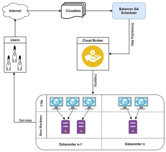
Figure 1. Abstract representation of the cloud environment.

3.2. Architecture of BGA

BGA is an enhanced GA for task scheduling, so the main structure has all major components of GA, as shown in Figure 2. BGA needs Size of Jobs in million instructions (mi) and computational Power of VMs in million instructions per second (mips). BGA begins with population initialization, and then the fitness against each chromosome is computed. Until stopping criteria are met, BGA keeps generating new chromosomes using crossover operators, which are then mutated, and a balancer operation is triggered after mutation. These components of BGA are explained one by one in detail. Table 1 provides the parameter settings of BGA, and Algorithm 1 presents the pseudocode of BGA.

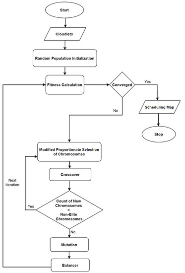
Figure 2. Flow diagram of the Balancer Genetic Algorithm (BGA).

Table 1. Parameter settings of BGA.

Parameters	Values
Population size	120
Iterations	1000
$\alpha$	0.18–0.22
$\beta$	0.75–0.85
$ϵ$	1.98–2.22
Mutation rate	0.0047

3.2.1. Encoding

In batch mode, the scheduler receives a number of tasks as an input, and then they have to be mapped. GA has chromosomes, and they need proper encoding to represent the task scheduling problem. There are multiple ways of encoding GA in task scheduling. BGA has discrete encoding, also known as real number encoding. Discrete encoding makes a vector of $1\times n$ dimension, where n is the number of tasks. It shows that for each task there is a corresponding value of genes representing the VM number. Genes have only one allele and whose range is the total number of VMs m.

Suppose there are six tasks that can be denoted as $T_1,T_2,T_3,T_4,T_5,T_6$. Tasks have to be mapped to three VMs represented as $R_1,R_2,R_3$. Let chromosomes be $v=3,2,3,1,2,2$. This implies that the $T_1$ is assigned to $R_3$. Similarly, $T_2$, $T_3$, $T_4$, $T_5$ and $T_6$ are mapped to $R_2$, $R_3$, $R_1$, $R_2$ and $R_2$, respectively. As there are three VMs, there are three pools of tasks. Here in the mapping defined for chromosome v, $R_1$ gets only one task, so the pool $R_1=\left\{T_4\right\}$, $R_2=\{T_2,T_5,T_6\}$ and $R_3=\{T_1,T_3\}$. The agenda of BGA is to find a chromosome representing a suitable mapping to meet the objectives of better makespan and load balancing.

Algorithm 1 BGA.

Input: Size of Jobs, Power of VMs      Output: Mapping of Jobs to VMs  1: $Population\left[\right]\leftarrow random\left(Num\text{\_}of\text{\_}VMs\right)$  2: for$i\leftarrow 0ton$do  3:      $load\text{\_}balancer\left[\right]\leftarrow LoadBalanceAlgorithm\left(Population\left[x_i\right]\right)$  4: end for  5: $SizePopulation\leftarrow size\left(Population\right[\left]\right)$  6: $s\leftarrow Half(SizePopulation-ϵ)$  7: $SinglePoint\leftarrow s\times \alpha$  8: $MultiPoint\leftarrow s\times \beta$  9: while GA does not converge do 10:     $newPopulation\leftarrow 0$ 11:     $p\leftarrow ϵ+1$ 12:     $Paren{t}_1\leftarrow 1$ 13:     $Paren{t}_2\leftarrow 1$ 14:     while $newPopulation<s$ do 15:         while $Paren{t}_1==Paren{t}_2$ do 16:               $Paren{t}_1\leftarrow SelectionAlgorithm\left(load\text{\_}balancer\left[\right]\right)$ 17:               $Paren{t}_2\leftarrow SelectionAlgorithm\left(load\text{\_}balancer\left[\right]\right)$ 18:         end while 19:         if $SinglePoint>1$ then 20:               $flag\leftarrow 1$ 21:               $Population\left[\right]\leftarrow CrossoverAlgorithm(Population\left[Paren{t}_1\right],Population\left[Paren{t}_2\right],flag,p)$ 22:         else 23:               $flag\leftarrow 2$ 24:               $Population\left[\right]\leftarrow CrossoverAlgorithm(Population\left[Paren{t}_1\right],Population\left[Paren{t}_2\right],flag,p)$ 25:         end if 26:         $SinglePoint\leftarrow SinglePoint-1$ 27:         $newPopulation\leftarrow newPopulation+1$ 28:     end while 29:     for $i\leftarrow 1toSizePopulation$ do 30:          if $Population\left[x_i\right]notBes{t}_{1}orBes{t}_2$ then 31:               $MutationAlgorithm\left(Population\left[x_i\right]\right)$ 32:         end if 33:     end for 34:     for $i\leftarrow 1toSizePopulation$ do 35:         $Population\left[x_i\right]\leftarrow BalancerAlgorithm\left(Population\left[x_i\right]\right)$ 36:     end for 37: end while

3.2.2. Fitness Function

BGA is a multi-objective technique to improve makespan and load balancing. Load balancing is achieved through a balancer operation described later. However, fitness function should measure the degree of improvement in both objectives. Hence, a multi-objective relation is unified to combine the effects of two separate inversely proportional objectives. Different mechanisms are opted to balance the load. In balancer GA a load balancing mechanism is inculcated, and the same becomes the basis for measuring the level of load balancing. The fitness function in which makespan and load balancing are combined is defined as:

$$L\left(x\right)=makespan+AvgPSU$$

(1)

where $0\le AvgPSU\le 1$ is an average of all percentage of shares used by all VMs for a specific chromosome and is calculated as follows:

$$AvgPSU=1-\frac{{\Sigma }_{j=1}^{n}PS{U}_j}{n}$$

(2)

The value of PSU is computed to find the share used by any VM; it depends on number of tasks assigned to any VM, and this assignment is represented through the genes of chromosome. $PS{U}_j$ is calculated for each VM, and $ShareUse{d}_j$ is the sum of the sizes of tasks assigned to VMj. $VMShar{e}_j$ is the maximum share in terms of million instructions that should be mapped to that VM ideally. $PS{U}_j$ is calculated as:

$$PS{U}_j=\frac{ShareUse{d}_j}{VMShar{e}_j}\times 100$$

(3)

In order to keep $PS{U}_j$ within $100\%$, we use:

$$\begin{array}{cc}\hfill if& (PS{U}_j>100)\hfill \\ & PS{U}_j=\frac{100-(PS{U}_j-100)}{100}\hfill \\ \hfill & \begin{array}{c}\hfill if(PS{U}_j<0)\\ & PS{U}_j=0\hfill \end{array}\hfill \\ \hfill else& \\ \hfill & PS{U}_j=\frac{PS{U}_j}{100}\hfill \end{array}$$

(4)

Equation (5) presents the formulation of $ShareUse{d}_j$ by any VM, and it is based on accumulated size of tasks assigned to that particular VM.

$$ShareUse{d}_j={\Sigma }_{i=1}^n(tasksiz{e}_i\times Map[i,j]),$$

(5)

where $Map[i,j]$ is a binary matrix that reflects the mapping of task ‘i’ to VM ‘j’, with 1 shows mapping and 0 shows no mapping.

Ideally a VM should obtain the size of tasks based on the computational power of VM in mips, i.e., $V{M}_j.mips$ as compared to other VMs. Furthermore, $ShareRati{o}_{\left(v{m}_j\right)}$ is a ratio that is used in the computation of maximum size of tasks in million instructions to be mapped to that $V{M}_j$. The following equations have been used to calculate these ratios:

$$VMShar{e}_j={\Sigma }_{i=1}^m\left(tas{k}_i\right)\times ShareRati{o}_{\left(v{m}_j\right)}$$

(6)

$$ShareRati{o}_{\left(v{m}_j\right)}=\frac{V{M}_j.mips}{{\Sigma }_{j=1}^n(V{M}_j.mips)}$$

(7)

Power of all available VMs is summed, and then the individual power of VM is divided by the sum of power to compute $ShareRati{o}_{(}v{m}_j)$. The fitness function in BGA, namely “LoadBalance”, is a minimization function, as makespan is a minimization value, and $AvgPSU$ is also converted accordingly as expressed already. The value of $AvgPSU$ is added to makespan, and it helps to find a solution where both objectives are improved. However, there is no advantage of better load balancing when makespan is not so good. To address this, additional information of load balancing is added to the value of makespan, and a novel load balancing mechanism is formulated. Algorithm 2 details the LoadBalance process devised by BGA.

3.2.3. Selection Operator

Proportionate selection operator with a few minor modifications has been incorporated in BGA. Proportionate selection relates to the spin of a roulette wheel, where the size of pie is a representation of worth of a specific chromosome among the entire population. In a normal proportionate selection operator, every chromosome has an opportunity to be selected. However, the fittest chromosomes have large proportions, and they can be selected more than others. In BGA, a minor modification is performed to eradicate the chances of extremely poor chromosomes from being selected repeatedly. Repeated selection of poor chromosomes does not contribute much to global search, and performance can also degrade. Therefore, the sum of LoadBalance is calculated, and after summation the LoadBalance value is converted to maximize only for the selection operation phase. Using proportionate selection, the chromosome with minimum LoadBalance gets the maximum proportion according to its fitness.

There are many possible ways to implement a proportionate selection operator. The steps used to perform proportionate selection in BGA with modification are as follows:

• Adding LoadBalance of chromosomes to compute the sum.
• Converting LoadBalance values of chromosome to maximization.
• Sorting chromosomes in decreasing order based on scaled LoadBalance values.
• Generating a random number $“r”$, where $1\le r\le sum$.
• Adding LoadBalance values to $“r”$ until $r\le sum$.

The last chromosome added is selected through the selection operator, and there are more chances to select the fittest as compared to others. Two chromosomes are selected through the selection operator, and then they participate in offspring generation. In the case when the same two chromosomes are selected as parents, the selection operation is repeated to select a different chromosome. Algorithm 3 provides the details of the selection process.

3.2.4. Crossover Operator

In BGA both single and multi-point crossover is performed. The probability of choosing a single point crossover “$\alpha$” is set to $20\%$, and for two points “$\beta$” is $80\%$. In this way, the population can have combined representation of single and multi-point crossovers. Single point crossover is more similar to parents, and two points adds some diversity; this increases the chances of incorporating a population with different combinations of best parent chromosomes to reach to a better solution. A random number n is generated, and if it is less than or equal to 0.2, new chromosomes are generated through single point, otherwise two-point crossover is performed. Two chromosomes selected through the selection operator generate two new chromosomes, and then the selection operator is triggered again until a set number of chromosomes are generated depending on the population size. The remaining chromosomes are moved as is to the next generation, and they behave as elite “$ϵ$” chromosomes. The top two fittest chromosomes are chosen as elites. The details of crossover are given in Algorithm 4.

Algorithm 2 LoadBalance.

Input: $Population\left[x_i\right]$      Output: $load\text{\_}balancer\left[x_i\right]$  1: procedureLoadBalanceAlgorithm  2:     $SizePopulation\leftarrow size\left(Population\right[\left]\right)$  3:     $JOBsum\leftarrow 0$  4:     $VMsum\leftarrow 0$  5:     $AvgPSU\leftarrow 0$  6:     for $i\leftarrow 1toJob\left[\right]$ do  7:         $JOBsum\leftarrow JOBsum+Job\left[x_i\right]$  8:     end for  9:     for $i\leftarrow 1toVM\left[\right]$ do 10:         $VMsum\leftarrow VMsum+VM\left[x_i\right]$ 11:   end for 12:   for $i\leftarrow 1toVM\left[\right]$ do 13:         $VMShare\leftarrow VM\left[x_i\right]/VMsum\times JOBsum$ 14:   end for 15:   for $i\leftarrow 1toSizePopulation$ do 16:         $VMmakespan\left[\right]\leftarrow 0$ 17:         for $j\leftarrow 1toGene\left[\right]$ do 18:            $VMmakespan\left[Gene\left[x_j\right]\right]\leftarrow VMmakespan\left[Gene\left[x_j\right]\right]+jobsize\left[x_j\right]$ 19:         end for 20:         for $k\leftarrow 1toVM\left[\right]$ do 21:               $value\leftarrow VMmakespan\left[k\right]/VMShare\left[k\right]\times 100$ 22:               if $value<=100$ then 23:                   $PSU\left[k\right]\leftarrow value/100$ 24:                else 25:                      $PSU\left[k\right]\leftarrow (100-(value-100\left)\right)/100$ 26:                end if 27:                $AvgPSU\leftarrow AvgPSU+PSU\left[k\right]$ 28:                $VMmakespan\left[k\right]\leftarrow VMmakespan\left[k\right]/Power\text{\_}of\text{\_}VM\left[k\right]$ 29:           end for 30:           $AvgPSU\leftarrow 1-AvgPSU$ 31:           $load\text{\_}balancer\left[x_i\right]\leftarrow Max\left(VMmakespan\left[\right]\right)+AvgPSU$ 32:     end for 33:     return $load\text{\_}balancer\left[x_i\right]$ 34: end procedure

Algorithm 3 Selection.

Input: $load\text{\_}balancer\left[\right]$      Output: $Population\left[x_i\right]$  1: procedureSelectionAlgorithm  2:     $SizePopulation\leftarrow size\left(Population\right[\left]\right)$  3:     $Sum\leftarrow sum\left(load\text{\_}balancer\right[\left]\right)$  4:     $r\leftarrow random\left(Sum\right)$  5:     $load\text{\_}balancer\left[\right]\leftarrow scale\left(load\text{\_}balancer\right[\left]\right)$  6:     $load\text{\_}balancer\left[\right]\leftarrow sort\left(load\text{\_}balancer\right[\left]\right)$  7:     $j\leftarrow 1$  8:     while $r<Sum$ do  9:           $r\leftarrow r+load\text{\_}balancer\left[x_j\right]$ 10:         $j\leftarrow j+1$ 11:     end while 12:     return $Population\left[x_j\right]$ 13: end procedure

3.2.5. Mutation Operator

Random resetting is used in BGA, and the mutation rate is set to 0.0047. This mutation rate is set experimentally by analyzing the standard deviation of the fitness value. The formulation of standard deviation is expressed as follows:

$$\sigma =\sqrt{\frac{{\Sigma }_{i=1}^n{(f\left(x_i\right)-\overline{f\left(x\right)})}^2}{k}}$$

(8)

where k is the size of the population. High standard deviation of fitness value shows that the population is too diversified, and the chance of focusing on a specific solution is very low. It is very hard to reach an optimal solution when deviation is high. On the other hand, when standard deviation is too low, it means that chromosomes are almost the same, and there is a need to introduce more diversity. With the help of standard deviation, a static mutation rate is selected that can better suit the need of the problem at hand.

There are different possible ways of performing the random resetting mutation. BGA generates a random number c where $0\le c\le 1$. The mutation probability is checked against each gene of the chromosome, and genes are mutated only if c is under the range of mutation rate. The mutation process details are provided in Algorithm 5.

3.2.6. Balancer Operator

After the generation of an entire population, for the next generation the balancer operation is performed. The goal of the balancer operation is to balance the workload among VMs. Tasks from overloaded VMs are migrated to underloaded and vice versa. The decision of over- and under-loaded VMs relies on the percentage of share used by any VM, just like one computed in the fitness function. Algorithm 6 shows the details of the balancer operator.

Algorithm 4 Crossover.

Input: $Population\left[Paren{t}_1\right],Population\left[Paren{t}_2\right],flag,p$      Output: $Population\left[x_i\right],Population\left[x_{i+1}\right]$  1: procedureCrossoverAlgorithm  2:     $SizeChromosome\leftarrow size\left(Population\left[x_i\right]\right)$  3:     $CutPoin{t}_1\leftarrow random\left(SizeChromosome\right)$  4:     $CutPoin{t}_2\leftarrow random\left(SizeChromosome\right)$  5:     if $flag==1$ then  6:           for $j\leftarrow 1toCutpoin{t}_1$ do  7:                 $Chil{d}_1\left[x_j\right]\leftarrow Population\left[Paren{t}_1\right]$  8:                 $Chil{d}_2\left[x_j\right]\leftarrow Population\left[Paren{t}_2\right]$  9:           end for 10:         for $j\leftarrow CutPoin{t}_1+1toSizeChromosome$ do 11:                 $Chil{d}_1\left[x_j\right]\leftarrow Population\left[Paren{t}_2\right]$ 12:                 $Chil{d}_2\left[x_j\right]\leftarrow Population\left[Paren{t}_1\right]$ 13:         end for 14:     else 15:         for $j\leftarrow 1toCutpoin{t}_1$ do 16:                 $Chil{d}_1\left[x_j\right]\leftarrow Population\left[Paren{t}_1\right]$ 17:                 $Chil{d}_2\left[x_j\right]\leftarrow Population\left[Paren{t}_2\right]$ 18:         end for 19:         for $j\leftarrow CutPoin{t}_1+1toCutPoin{t}_2$ do 20:                 $Chil{d}_1\left[x_j\right]\leftarrow Population\left[Paren{t}_2\right]$ 21:                 $Chil{d}_2\left[x_j\right]\leftarrow Population\left[Paren{t}_1\right]$ 22:         end for 23:         for $j\leftarrow CutPoin{t}_2+1toSizeChromosome$ do 24:                 $Chil{d}_1\left[x_j\right]\leftarrow Population\left[Paren{t}_1\right]$ 25:                 $Chil{d}_2\left[x_j\right]\leftarrow Population\left[Paren{t}_2\right]$ 26:         end for 27:     end if 28:     $Population\left[p\right]\leftarrow Chil{d}_1\left[\right]$ 29:     $p\leftarrow p+1$ 30:     $Population\left[p\right]\leftarrow Chil{d}_2\left[\right]$ 31:     $p\leftarrow p+1$ 32:     return $Population[p-2]$, $Population[p-1]$ 33: end procedure

Algorithm 5 Mutation.

Input: $Population\left[x_i\right]$      Output: $Population\left[x_i\right]$  1: procedureMutationAlgorithm  2:     $SizeChromosome\leftarrow size\left(Population\left[x_i\right]\right)$  3:     for $i\leftarrow 1toSizeChromosome$ do  4:           $r\leftarrow random\left(1\right)$  5:           if $r<=probability$ then  6:                 $r\leftarrow random\left(SizeChromosome\right)$  7:                $Gene\left[x_i\right]\leftarrow r$  8:         end if  9:     end for 10:   return 11: end procedure

Algorithm 6 Balancer.

Input: $Population\left[x_i\right]$      Output: $Population\left[x_i\right]$  1: procedureBalancerAlgorithm  2:     $SizeChromosome\leftarrow size\left(Population\left[x_i\right]\right)$  3:     for $i\leftarrow 1toSizeChromosome$ do  4:         if $VMShare\left[Gene\left[x_i\right]\right]>0$ then  5:            $VMShare\left[Gene\left[x_i\right]\right]\leftarrow VMShare\left[Gene\left[x_i\right]\right]-JobSize\left[x_i\right]$  6:            if $VMShare\left[Gene\left[x_i\right]\right]<0$ then  7:                $VMShare\left[Gene\left[x_i\right]\right]\leftarrow VMShare\left[Gene\left[x_i\right]\right]+JobSize\left[x_i\right]$  8:                $list\left[\right]\leftarrow jobID$  9:            end if 10:         end if 11:     end for 12:     $Jobs\left[\right]\leftarrow sort\left(Jobs\right)$ 13:     $VMShare\leftarrow sort\left(VMShare\right)$ 14:     while $list\left[\right]notempty$ do 15:         while $VMShare\left[max\right]>0$ do 16:            $VMShare\left[max\right]\leftarrow VMShare\left[max\right]-Job\left[list\left[x_i\right]\right]$ 17:            $Population\left[Job\left[x_i\right]\right]\leftarrow VMnumber$ 18:         end while 19:     end while 20:     return $Population\left[x_i\right]$ 21: end procedure

The balancer operation is performed on each chromosome of the population, except for the elite chromosomes. The major advantage of this balancer operator, as compared to other techniques, is that it does not totally change the chromosome. Other techniques modify a significant number of genes, which may not be as helpful because the chromosome loses its actual characteristics. Other techniques also do not check the VM share information to recognize the over- and under-loaded VMs.

The chromosome becomes an input of the balancer operator, and genes of the chromosome are traversed. The total VM share of each VM is already computed before fitness is computed, and it is also utilized in the balancer operator. As the value of a gene represents a VM number corresponding to a task, the VM share is checked against each gene of the chromosome. Initially, the share of every VM is at maximum according to their VM share. While traversing the genes of the chromosome, the size of the task is subtracted from the respective VM. If the VM share is greater than 0, it means that the task can be assigned to the VM, and the size of the task is subtracted on assignment. Otherwise, if the VM share is less than or equal to 0, it means that VM is over-loaded and there is no need to assign any other task to that VM. In such cases, the task being assigned is added to a pool of tasks known as $cloudle{t}_{pool}$. After the assignment, if the VM share drops below 0 the respective task is added to a pool of tasks, which is later used in remapping. After the traversal of the last gene, VMs are sorted according to their remaining VM share in $V{M}_{pool}$. Tasks in $cloudle{t}_{pool}$ are also sorted in descending order. The maximum sized task in the task pool is mapped to VM with the maximum remaining VM share. The $cloudle{t}_{pool}$ and $v{m}_{pool}$ both are updated accordingly. This process of remapping continues until there are no remaining tasks in $cloudle{t}_{pool}$.

3.2.7. Fusion of Heuristic

A load balancing mechanism is embedded in GA to have the tendency of load balancing in a chromosome. This provides additional guidance to GA. Using a heuristic just at the initialization phase cannot have a significant impact. The benefit of fusing the balancer mechanism is that it balances the chromosomes based on their VM share. BGA explores the large search space where there are many possible solutions. Consequently, a large number of chromosomes pass through the balancer operation. It is possible to explore many solutions in which the load balancing is the same, but the fitness value varies according to their makespan, and this could not be achieved otherwise.

4. Performance Metrics

To evaluate the performance of BGA, we compared it with benchmark techniques. To this end, the following performance metrics are used:

4.1. Makespan

Makespan is the finishing time of batch of tasks and is calculated as:

$$\begin{array}{c}makespan=max\left(CT\text{\_}VM\text{\_}j\right),\\ j=1,2,\dots ,n\end{array}$$

(9)

where $CT$ is the completion time of a specific VM, and the maximum time taken by any VM is the makespan.

4.2. ARUR

ARUR is the average resource utilization ratio, and it is between 0 and 1, where 0 represents minimum and 1 maximum resource utilization. It is computed through completion time as:

$$ARUR=\frac{\left({\sum }_{j=1}^{n}C{T}_{V{M}_j}\right)/n}{makespan}$$

(10)

5. Experimental Results and Discussion

This section details the experimental setup and dataset used in the experimentation. The benchmark techniques are also defined, and then the results are expressed with necessary discussion.

5.1. Experimental Setup

CloudSim [37] is used to simulate the cloud-based environment for experimentation. All experiments are performed using the same settings mentioned for the benchmark techniques. However, the number of iterations are fixed to 1000 for all meta-heuristic techniques as a stopping criterion. One data center is created in cloudsim. The data center has 30 host machines and a total of 50 VMs. The RAM of host machines is 16,384 MBs. Host machines have a Linux Operating System, and 4 machines are dual-core whereas 26 machines are Quad-core. Dual and Quad-core machines have processing power of 4000 MIPS. The space sharing VM scheduling algorithm of CloudSim is used for experimentation. The processing power of 50 heterogeneous VMs is detailed in Table 2.

Table 2. Power of VMs in experimentation.

VM No.	Power (MIPS)	VM No.	Power (MIPS)
1–7	100	27-32	1250
8–14	500	33-38	1500
15–20	750	39-44	1750
21–26	1000	45-50	4000

5.2. Workload Generation

A synthetic dataset [2,24] is used, and it has four different categories which are defined as follows:

• Left Skewed: Large-sized tasks are numerous.
• Right Skewed: Small-sized tasks are numerous.
• Normal: Small- and large-sized tasks are almost equal in number.
• Uniform: Tasks are of almost same sizes.

These four categories can better express the overall behavior of BGA on different possible workloads. Each category has batches of 100, 200, 300, 400, 500, 600, 700, 800, 900 and 1000 tasks.

5.3. Benchmark Techniques

Table 3 lists the baseline techniques used for the performance evaluation. MGGS [13] is selected because it has a load balancing mechanism embedded in GA. BGA also has the same method of fusing the load balancing mechanism, but the working of GA and the mechanism of load balancing are unique. ETA-GA [18] is compared as it is a pure GA-based technique. DSOS [24] is a meta-heuristic, and RALBA [3] is a state-of-the-art heuristic technique. All of these techniques are compared with BGA.

Table 3. Benchmark Techniques.

Techniques	Performance Metrics Demonstrated
MGGS [13]	Load balancing and makespan
ETA-GA [18]	Makespan and network failure
RALBA [3]	Load balancing, throughput and makespan
DSOS [24]	Load balancing, makespan, response time and convergence

5.4. Discussion on the Comparison

Figure 3 shows the makespan values on the left—skewed dataset. In almost all batch sizes BGA performs better. However, MGGS and RALBA are close competitors. On average, overall, BGA achieved 27.3, 71.9, 40.5 and 4.6% improvement in makespan compared with MGGS, ETA-GA, DSOS and RALBA, respectively. For a small batch size of 100, RALBA slightly surpasses BGA in makespan. Still, for large batch sizes, which are more realistic for cloud systems, BGA outperforms all the benchmark techniques. Figure 4 shows the results of makespan on a right—skewed dataset. BGA has achieved 19.8, 72.2, 42.4 and 3.2% average improvement in makespan compared with MGGS, ETA-GA, DSOS and RALBA, respectively.

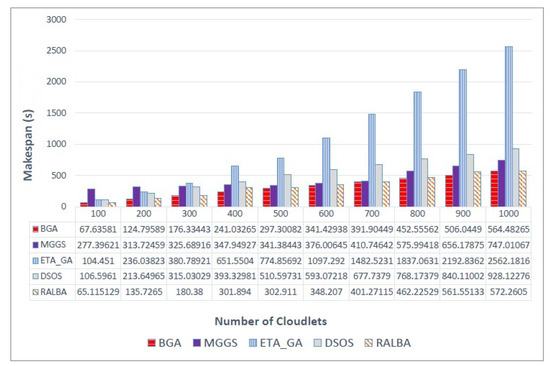
Figure 3. Makespan results on the left—skewed dataset.

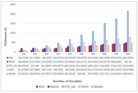
Figure 4. Makespan results on the right—skewed dataset.

Similarly, Figure 5 shows makespan value on a normal dataset. BGA has attained better makespan with average improvement of 23.3, 72.1, 41.6 and 5.9% as compared to MGGS, ETA-GA, DSOS and RALBA, respectively. Finally, improvement of BGA on the uniform dataset is reflected in Figure 6. BGA performed 19.2, 71.9, 42.1 and 6.7% better in makespan than MGGS, ETA-GA, DSOS and RALBA, respectively.

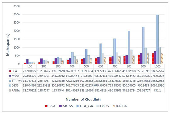
Figure 5. Makespan results on the normal dataset.

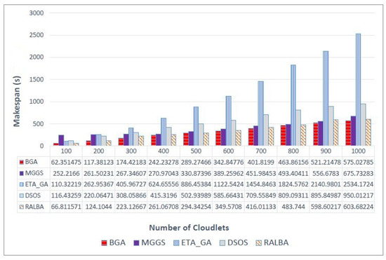
Figure 6. Makespan results on the uniform dataset.

It is evident that, overall, on all categories and batch sizes of datasets, BGA outperforms. Specifically for the uniform dataset, RALBA was a close competitor and deteriorated to highest level of 6.7%. Even if MGGS is close at some points, MGGS is more computationally expensive than other meta-heuristics compared here, so it is not a right choice to consider, especially where time is concerned.

There are different ways to measure load balancing, and ARUR is a very popular one of them. The value of ARUR is between 0 and 1, but it can signify the percent of workload balance. BGA is a load balancing technique. Therefore, this QoS parameter is very important for the claim of better load balancing. On left—skewed dataset the load balancing achieved is shown in Figure 7. At batch size 500, MGGS performs better; for a small batch size of 100, RALBA performs better. The average improvement of BGA over MGGS, ETA-GA, DSOS and RALBA in terms of load balancing is 5.2, 77, 60.6 and 5.4%, respectively. MGGS, DSOS and RALBA are the techniques that have reported better load balancing. Out of these, only RALBA and MGGS have deployed a load balancing mechanism in their approach. Here again, just like makespan, RALBA is a close competitor of BGA in load balancing. However, the results show that, on average, 5.4% better load balancing is achieved on left—skewed and likewise other datasets. On the right—skewed dataset the improvement in ARUR is shown in Figure 8. BGA has attained 12.5, 89.5, 70.1 and 6.1% better ARUR than MGGS, ETA-GA, DSOS and RALBA, respectively. At a batch size of 400, MGGS performs better, but generally it does not perform better than BGA. Figure 9 shows results of ARUR on a normal dataset. Here, BGA has achieved 12.5, 82.2, 65.2 and 6% better load balancing as compared to MGGS, ETA-GA, DSOS and RALBA, respectively. Similarly, on the uniform dataset BGA again performs better than MGGS, ETA-GA, DSOS and RALBA with the improvement of 12.5, 82.2, 65.2 and 6%, respectively, as expressed in Figure 10. Load balancing of BGA is highest as compared to RALBA, a close competitor on the right—skewed dataset. Generally, it is observed that for batch sizes of 400 and 500, at some places MGGS performs better, but it has the overhead of too much time for load balancing. Overall, BGA outperforms in load balancing than all other techniques.

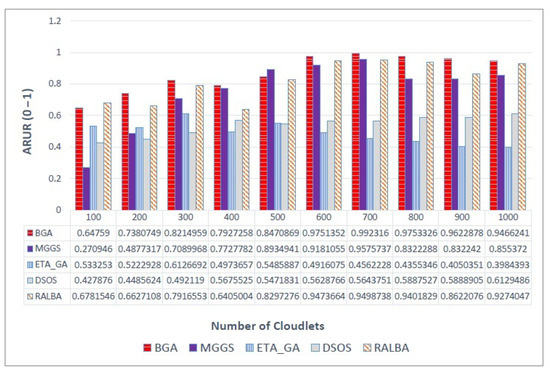
Figure 7. ARUR results on the left—skewed dataset.

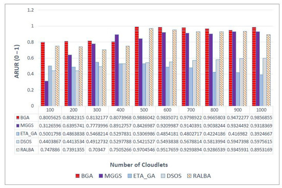
Figure 8. ARUR results on the right—skewed dataset.

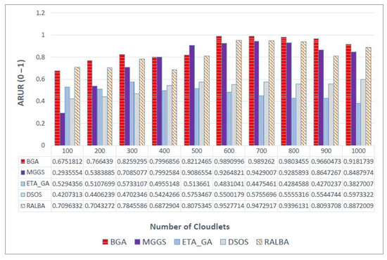
Figure 9. ARUR results on the normal dataset.

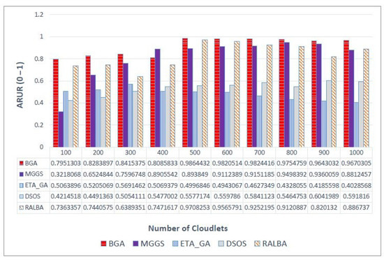
Figure 10. ARUR results on the uniform dataset.

Throughput is the number of tasks computed in a unit time, so it depends on the makespan value. Thus, when makespan is good, it is evident that throughput would also be good. According to the claim of this research, BGA has better throughput than MGGS, ETA-GA, DSOS and RALBA. Figure 11, Figure 12, Figure 13 and Figure 14 show the throughput of BGA and other techniques on left—skewed, right—skewed, normal and uniform datasets, respectively. On the left—skewed dataset the improvement is 29.7, 64, 40 and 4.6% over MGGS, ETA-GA, DSOS and RALBA, respectively. On the right—skewed dataset 24.1, 65.4, 43 and 4% improvement in throughput is achieved as compared to MGGS, ETA-GA, DSOS and RALBA, respectively. On the normal dataset 26.1, 64.4, 41.7 and 5.1% improvement is achieved over MGGS, ETA-GA, DSOS and RALBA, respectively. On the uniform dataset 23.4, 65.5, 42.9 and 6.9% improvement is achieved over MGGS, ETA-GA, DSOS and RALBA, respectively.

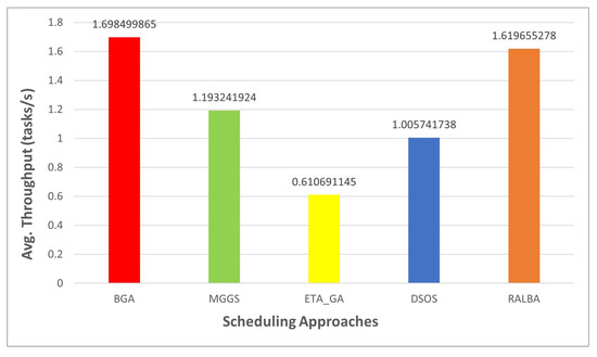
Figure 11. Average throughput results on the left—skewed dataset.

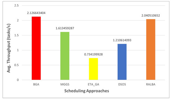
Figure 12. Average throughput results on the right—skewed dataset.

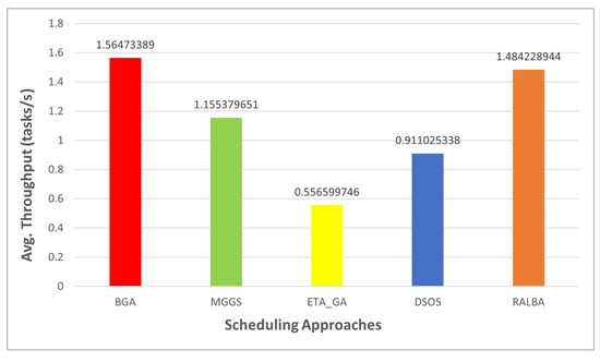
Figure 13. Average throughput results on the normal dataset.

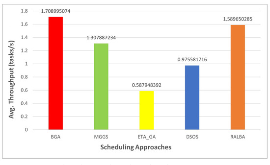
Figure 14. Average throughput results on the uniform dataset.

6. Conclusions

In this research, state-of-the-art heuristic and meta-heuristic task schedulers are analyzed in depth, and it is determined that scheduling results in inefficient load balancing of cloud resources. The need for multi-objective optimization is expressed as a motivation, where load balancing serves as a significant metric parallel to makespan for efficient task scheduling. For exploration of a large search space of possible solutions, meta-heuristics are opted for, and when heuristics are merged, an additional capability to explore more optimal solutions is complemented.

In this work, a novel task scheduling technique is presented, namely Balancer Genetic Algorithm (BGA), to improve makespan and load balancing. A load balancing mechanism is fused in GA with other necessary tuning of parameters to achieve better results. Formulations of multi-objective fitness functions are expressed in detail. CloudSim is used as a platform for simulating the behavior of presented techniques in a cloud data center, where resources and tasks to be mapped on resources are heterogeneous. Rigorous experiments are performed to demonstrate that BGA outperforms state-of-the-art MGGS, ETA-GA, DSOS and RALBA schedulers for performance measures of makespan, throughput and load balancing. Heterogeneous distribution of workload with varying batches of tasks is used to avoid biased dataset-dependent experimentation.

Currently, BGA does not cater to Service Level Agreements to prioritize tasks having dependency. In the future, BGA can be extended to incorporate Service Level Agreements where tasks have unequal priorities.

References

- Fang, Y.; Xiao, X.; Ge, J. Cloud Computing Task Scheduling Algorithm Based On Improved Genetic Algorithm. In Proceedings of the 2019 IEEE 3rd Information Technology, Networking, Electronic and Automation Control Conference (ITNEC), Chengdu, China, 15–17 March 2019; pp. 852–856. [Google Scholar] [CrossRef]
- Abdullahi, M.; Ngadi, M.A.; Dishing, S.I.; Ahmad, B.I.E. An efficient symbiotic organisms search algorithm with chaotic optimization strategy for multi-objective task scheduling problems in cloud computing environment. J. Netw. Comput. Appl. 2019, 133, 60–74. [Google Scholar] [CrossRef]
- Hussain, A.; Aleem, M.; Khan, A.; Iqbal, M.A.; Islam, M.A. RALBA: A computation-aware load balancing scheduler for cloud computing. Cluster Comput. 2018, 21, 1667–1680. [Google Scholar] [CrossRef]
- Gong, C.; Liu, J.; Zhang, Q.; Chen, H.; Gong, Z. The characteristics of cloud computing. In Proceedings of the 2010 39th International Conference on Parallel Processing Workshops, San Diego, CA, USA, 13–16 September 2010; pp. 275–279. [Google Scholar] [CrossRef]
- Duan, K.; Fong, S.; Siu, S.W.I.; Song, W.; Guan, S.S.-U. Adaptive Incremental Genetic Algorithm for Task Scheduling in Cloud Environments. Symmetry 2018, 10, 168. [Google Scholar] [CrossRef]
- Wang, Y.; Zuo, X. An Effective Cloud Workflow Scheduling Approach Combining PSO and Idle Time Slot-Aware Rules. IEEE/CAA J. Autom. Sin. 2021, 8, 1079–1094. [Google Scholar] [CrossRef]
- Xu, Z.; Xu, X.; Zhao, X. Task scheduling based on multi-objective genetic algorithm in cloud computing. J. Inf. Comput. Sci. 2015, 1429–1438. [Google Scholar] [CrossRef]
- Panda, S.K.; Jana, P.K. Load balanced task scheduling for cloud computing: A probabilistic approach. Knowl. Inf. Syst. 2019, 61, 1607–1631. [Google Scholar] [CrossRef]
- Mansouri, N.; Zade, B.M.H.; Javidi, M.M. Hybrid task scheduling strategy for cloud computing by modified particle swarm optimization and fuzzy theory. Comput. Ind. Eng. 2019, 130, 597–633. [Google Scholar] [CrossRef]
- Ebadifard, F.; Babamir, S.M. A PSO-based task scheduling algorithm improved using a load-balancing technique for the cloud computing environment. Concurr. Comput. Pract. Exp. 2018, 30, e4368. [Google Scholar] [CrossRef]
- Hussain, A.; Aleem, M.; Iqbal, M.A.; Islam, M.A. SLA-RALBA: Cost-efficient and resource-aware load balancing algorithm for cloud computing. J. Supercomput. 2019, 75, 6777–6803. [Google Scholar] [CrossRef]
- Manglani, V.; Jain, A.; Prasad, V. Task scheduling in cloud computing. Inter. J. Adv. Res. Comput. Sci. 2018, 821–825. [Google Scholar] [CrossRef]
- Zhou, Z.; Li, F.; Zhu, H.; Xie, H.; Abawajy, J.H.; Chowdhury, M.U. An improved genetic algorithm using greedy strategy toward task scheduling optimization in cloud environments. Neural Comput. Appl. 2019, 1–11. [Google Scholar] [CrossRef]
- Kaur, S.; Verma, A. An efficient approach to genetic algorithm for task scheduling in cloud computing environment. Int. J. Inf. Technol. Comput. Sci. (IJITCS) 2012, 4, 74. [Google Scholar] [CrossRef]
- Mohamad, Z.; Mahmoud, A.A.; Nik, W.N.S.W.; Mohamed, M.A.; Deris, M.M. A genetic algorithm for optimal job scheduling and load balancing in cloud computing. Inter. J. Eng. Technol. 2018, 290–294. [Google Scholar] [CrossRef]
- Hamad, S.A.; Omara, F.A. Genetic-based task scheduling algorithm in cloud computing environment. Int. J. Adv. Comput. Sci. Appl. 2016, 7, 550–556. [Google Scholar] [CrossRef]
- Zhan, Z.H.; Zhang, G.Y.; Gong, Y.J.; Zhang, J. Load balance aware genetic algorithm for task scheduling in cloud computing. In Proceedings of the Asia-Pacific Conference on Simulated Evolution and Learning, Dunedin, New Zealand, 15–18 December 2014; pp. 644–655. [Google Scholar] [CrossRef]
- Rekha, P.M.; Dakshayini, M. Efficient task allocation approach using genetic algorithm for cloud environment. Clust. Comput. 2019, 22, 1241–1251. [Google Scholar] [CrossRef]
- Javanmardi, S.; Shojafar, M.; Amendola, D.; Cordeschi, N.; Liu, H.; Abraham, A. Hybrid job scheduling algorithm for cloud computing environment. In Proceedings of the Fifth International Conference on Innovations in Bio-Inspired Computing and Applications IBICA 2014, Ostrava, Czech Republic, 23–25 June 2014; pp. 43–52. [Google Scholar] [CrossRef]
- Kokilavani, T.; Amalarethinam, D.G. Load balanced min-min algorithm for static meta-task scheduling in grid computing. Int. J. Comput. Appl. 2011, 20, 43–49. [Google Scholar] [CrossRef]
- Alnusairi, T.S.; Shahin, A.A.; Daadaa, Y. Binary PSOGSA for Load Balancing Task Scheduling in Cloud Environment. Int. J. Adv. Comput. Sci. Appl. 2018. [Google Scholar] [CrossRef]
- Abdi, S.; Motamedi, S.A.; Sharifian, S. Task scheduling using modified PSO algorithm in cloud computing environment. In Proceedings of the International Conference on Machine Learning, Electrical and Mechanical Engineering, Tomsk, Russia, 16–18 October 2014; Volume 4, pp. 8–12. [Google Scholar]
- Cao, Y.; Zhang, H.; Li, W.; Zhou, M.; Zhang, Y.; Chaovalitwongse, W.A. Comprehensive learning particle swarm optimization algorithm with local search for multimodal functions. IEEE Trans. Evol. Comput. 2018, 23, 718–731. [Google Scholar] [CrossRef]
- Abdullahi, M.; Ngadi, M.A. Symbiotic Organism Search optimization based task scheduling in cloud computing environment. Future Gener. Comput. Syst. 2016, 56, 640–650. [Google Scholar] [CrossRef]
- Nasr, A.A.; El-Bahnasawy, N.A.; Attiya, G.; El-Sayed, A. Using the TSP solution strategy for cloudlet scheduling in cloud computing. J. Netw. Syst. Manag. 2019, 27, 366–387. [Google Scholar] [CrossRef]
- Panda, S.K.; Jana, P.K. An energy-efficient task scheduling algorithm for heterogeneous cloud computing systems. Clust. Comput. 2019, 22, 509–527. [Google Scholar] [CrossRef]
- Singh, S.; Kalra, M. Scheduling of independent tasks in cloud computing using modified genetic algorithm. In Proceedings of the 2014 International Conference on Computational Intelligence and Communication Networks, Bhopal, India, 14–16 November 2014; pp. 565–569. [Google Scholar] [CrossRef]
- Kaur, S.; Sengupta, J. Load Balancing using Improved Genetic Algorithm (IGA) in Cloud computing. Int. J. Adv. Res. Comput. Eng. Technol. (IJARCET) 2017, 6. [Google Scholar]
- Kumar, A.S.; Venkatesan, M. Multi-Objective Task Scheduling Using Hybrid Genetic-Ant Colony Optimization Algorithm in Cloud Environment. Wirel. Pers. Commun. 2019, 107, 1835–1848. [Google Scholar] [CrossRef]
- Krishnasamy, K. Task scheduling algorithm based on hybrid particle swarm optimization in cloud computing environment. J. Theor. Appl. Inf. Technol. 2013, 55, 33–38. [Google Scholar]
- Kaur, G.; Sharma, E.S. Optimized utilization of resources using improved particle swarm optimization based task scheduling algorithms in cloud computing. Int. J. Emerg. Technol. Adv. Eng. 2014, 4, 110–115. [Google Scholar]
- Beegom, A.A.; Rajasree, M.S. Integer-PSO: A discrete PSO algorithm for task scheduling in cloud computing systems. Evol. Intell. 2019, 12, 227–239. [Google Scholar] [CrossRef]
- Bitam, S. Bees life algorithm for job scheduling in cloud computing. In Proceedings of the Third International Conference on Communications and Information Technology, Coimbatore, India, 26–28 July 2012; pp. 186–191. [Google Scholar] [CrossRef]
- Awad, A.I.; El-Hefnawy, N.A.; Abdel_kader, H.M. Enhanced particle swarm optimization for task scheduling in cloud computing environments. Procedia Comput. Sci. 2015, 65, 920–929. [Google Scholar] [CrossRef]
- Rjoub, G.; Bentahar, J.; Abdel Wahab, O.; Bataineh, A.S. Deep and reinforcement learning for automated task scheduling in large-scale cloud computing systems. Concurr. Comput. Pract. Exp. 2020, e5919. [Google Scholar] [CrossRef]
- Sharma, M.; Garg, R. An artificial neural network based approach for energy efficient task scheduling in cloud data centers. Sustain. Comput. Inform. Syst. 2020, 26, 100373. [Google Scholar] [CrossRef]
- Calheiros, R.N.; Ranjan, R.; Beloglazov, A.; De Rose, C.A.; Buyya, R. CloudSim: A toolkit for modeling and simulation of cloud computing environments and evaluation of resource provisioning algorithms. Softw. Pract. Exp. 2011, 41, 23–50. [Google Scholar] [CrossRef]
Publisher’s Note: MDPI stays neutral with regard to jurisdictional claims in published maps and institutional affiliations. |
© 2021 by the authors. Licensee MDPI, Basel, Switzerland. This article is an open access article distributed under the terms and conditions of the Creative Commons Attribution (CC BY) license (https://creativecommons.org/licenses/by/4.0/).