Abstract
This paper proposes a nonlinear decoupled current control scheme for a grid-connected inverter with LCL filter. Decoupling the active and reactive current control channels is one of the main demands in the control of inverters. For inverters with an L filter, the decoupling can be achieved by a proper feed-forward of grid voltages. However, the coupling of channels is a complex issue for converters with LCL filters. The resonance mode of the LCL filter may cause instability, which adds more complexity to the analysis. In this paper, state equations of the system are provided, which highlight the coupling between active and reactive currents injected into the grid. Accordingly, a non-linear control scheme is proposed which effectively decouples the channels and dampens the resonant modes of the LCL filter. The stability of the proposed control method is verified by the Lyapunov criterion. Independency of the system stability to the grid-impedance is another feature of the proposed approach. Moreover, only grid-side currents are needed for implementation of the proposed scheme, avoiding the need for additional current sensors for the output capacitor and grid-side inductor. For accurate modelling of the inverter, the computation and PWM sampling delays are included in the controller design. Finally, various case studies are provided that verify the performance of the proposed approach and the stability of the system.
1. Introduction
Voltage source converters (VSCs) are widely used in modern power systems for the integration of renewable energies, distributed power generation, energy storage systems, electric vehicle chargers, high and medium voltage transmission systems, hybrid AC/DC microgrids, motor derive systems, DC homes, etc. [1,2]. Apart from significant benefits coming from the usage of VSCs, their switching-based operation yields to harmonically polluted output voltages, which consequently creates harmonic currents injected into the grid. International standards have provided restrictions on the harmonic content, which are normally satisfied by adding harmonic filters in the output of the inverters. For this purpose, standard types of L and LCL filters are well defined in the literature [3]. Comparing filters, the LCL-filter is superior in terms of filter size, weight, and harmonic attenuation performance [4]. Using an LCL-filter is more common in high power applications, in which the switching frequency is lowered to reduce switching losses and VSC cost. However, the controller design in the presence of an LCL filter is more complicated, which is discussed in this paper.
In most applications, the control of DC-link voltage and reactive power are implemented in the control structure of the VSCs. In this structure, the concept of cascaded a control loop scheme is employed, in which the DC-link voltage and reactive power control loops are outer loops, and the control loops of the output currents are inner loops. Using an LCL filter introduces two challenges in the current control loop: (i) introducing resonant modes of an LCL filter, which impairs the stability of the whole converter system, and (ii) strong coupling between active and reactive currents, which impairs their independent control. In the following, the existing solutions for both challenges are provided.
1.1. Damping the Resonant Modes
Appearing resonant modes in the system is the first challenge introduced by employing LCL-filters. In the existing studies, two general approaches have been proposed for damping the resonance modes: (i) passive damping (PD) and (ii) active damping (AD). In the PD method, an extra series or parallel resistor is added to the filter elements. This damping method is simple; however, it increases power loss. Alternatively, AD methods dampen resonant modes by employing proper control algorithms, which are efficient and cost effective [2]. Various AD methods have been presented in literature, which are generally categorized into two groups of (i) filter-based (single loop) and (ii) feedback-based (multi loop) methods [5].
In filter-based methods, only grid-side or inverter-side current is measured, and the resonant modes are dampened using proper control schemes. This method is called the single loop cascade control method [6,7,8]. The filter-based methods are usually implemented by a notch filter with the characteristic frequency equal to the resonant frequency. This method does not demand an extra sensor, which makes it cost effective. However, its performance, stability margin, and robustness are not acceptable, and the dependency of the scheme on the resonant mode frequency and the variation of the filter parameters intensifies the mentioned deficiencies [5,9]. Meanwhile, the bandwidth of the control feedback should be low enough and should be reduced to about of the resonance frequency [10]. This is a large deficiency, especially in systems with low-resonance frequency. In feedback-based methods, in addition to using the state variable of grid-side current, other state variables are used in the control loop, which is known as the multi loop method. In this method, the output capacitor current [11,12,13], the output capacitor voltage [14], the inverter-side current [15,16], and combination of multiple states [4,17,18] are utilized as inner loop feedback signals. Among the different feedback signals, capacitor current and inverter-side current provide superior stability characteristics for resonance damping with simple implementation.
Further to the filter-based and feedback-based methods, predictive control [19,20,21,22], robust control [23,24,25], adaptive control [26,27], and predictive adaptive robust control [28] have also been presented in the literature. However, the complexity of the schemes has limited the practical implementation of these control schemes.
1.2. Decoupling of Active and Reactive Powers
Knowing that the DC-linked voltage control of grid-connected inverters is performed via the active current control channel, and reactive power injection is achieved by the reactive current control channel, the decoupling of the active and reactive current channels is a necessary demand to improve the system’s overall performance and independent control of the active and the reactive powers [25]. In an inverter with an L filter, the decoupling between active and reactive power in a synchronous dq frame is achieved by feed-forward signals into the current control loop. In inverters with an LCL filter, the control system is a multi-input-multi-output (MIMO) system (2 input-2 output) with tight coupling between channels; a simple feed-forward scheme cannot provide sufficient decoupling for the system [29]. Further to the above-mentioned importance of decoupling, the potential instability issue is another aspect which necessitates the channels decoupling for MIMO systems [29]. In other words, the strong coupling between channels in MIMO systems may cause instability of the system and should be avoided. To tackle this issue, a pre-controller based on the multivariable control theory is used to decrease coupling, which makes the system column or row dominant. However, the pre-controller cannot guarantee complete decoupling [29].
To compare the different existing approaches, Table 1 is provided. In this table, the available methods in the literature are compared considering different aspects, including (i) decoupled control of active and reactive currents, (ii) stability margin and resonance damping capability, (iii) the number of needed sensors, and (iv) complexity and order of controller. Also, the proposed method is included in this table, and the results of comparison show the superiority of the proposed method compared to existing methods. It should be mentioned that all characteristics of the proposed method, indicated in Table 1, are demonstrated in theory and simulation throughout the rest of the paper.

Table 1.
Different active damping control schemes for a grid-connected inverter with LCL-filter.
As a conclusion for the above propositions, to the best of the authors knowledge, there is a lack of a suitable control scheme which simultaneously considers both demands of (i) damping the resonant modes and (ii) the decoupling of active and reactive powers for inverters with an LCL filter. Keeping the number of sensors at minimum is another required criterion. This paper proposes a non-linear control method for a grid-connected inverter with an LCL filter that satisfies both requirements. In the proposed scheme, the minimum number of sensors is used since only grid-side currents are measured directly, and inverter-side currents and capacitor voltages are estimated using a reduced-order Luenberger observer. Having less sensors, in addition to cost reduction, can improve system reliability. Furthermore, a new scheme is presented to determine the phase margin (PM) of current control loop. The computational and PWM delays are included in the in tuning of current control loops.
Based on the above explanations, the objectives of the paper are as follows:
- the decoupling of active and reactive current channels and corresponding independent control of active and reactive powers;
- effective damping of resonant modes caused by an LCL-filter;
- using the minimum number of sensors, leading to cost reduction and improved system reliability;
- developing a parameter-tuning approach for the studied MIMO system using well-known criteria of phase and gain margin;
- consideration of computational and PWM delays in the control loop and controller parameters tuning.
This paper is organized as follows: the next section presents the modeling of the VSCs with an LCL filter in a dq reference frame; in Section 3, the proposed current controller is explained as well as an estimation of LCL filter-state variables and explanation of DC-link voltage and reactive power control loops; in Section 4, a phase margin determination scheme is presented, which provides a systematic method for tuning the proposed current control parameters; performance of the final controlled system in different situations is evaluated through different case studies in Section 5; finally, Section 6 concludes the paper.
2. Modeling of Grid Connected Inverter with LCL Filter
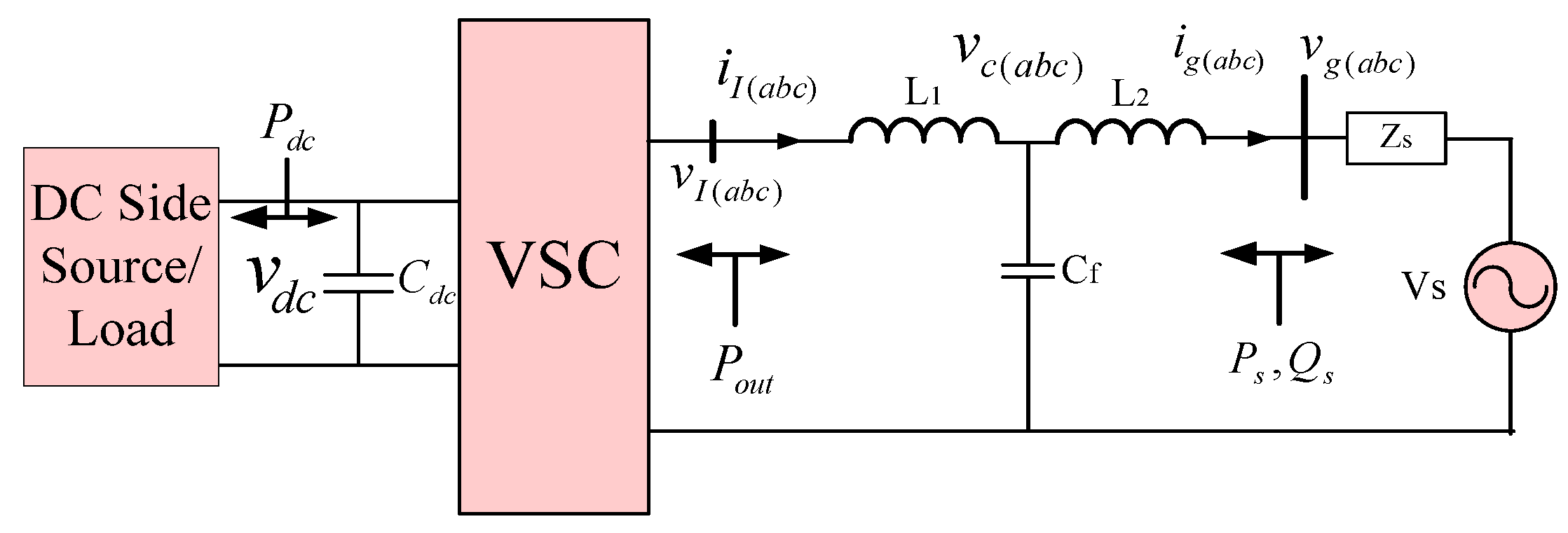
Figure 1 shows the single line diagram of a three-phase grid-connected VSC with an LCL filter [30,31]. In this figure, the grid is modelled by its Thevenin equivalent. The dynamic equations of the system including AC part and DC link is presented:
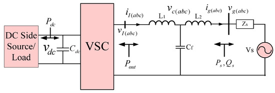
Figure 1.
Single line diagram of a three-phase grid-connected VSC with LCL filter.
All parameters are depicted in Figure 1.
To remove the nonlinearity on the left-hand side of the DC-link voltage dynamic Equation (4), the energy stored in the DC link capacitor, , is used as an alternative variable [32]. Then, (4) can be rewritten as:
Using a phase-locked loop (PLL) for extraction of angular frequency of , and applying Park transformation to the state equations of (1) and (5) yields:
In the equations, (, ) and (, ) are currents flowing through inductors and , respectively; (, ) are voltages across the output filter capacitor, (, ) are inverter terminal voltages, and (, ) are PCC voltages, all in dq frame. Also, is a nonlinear term which shows the instantaneous power absorbed by the elements of the LCL filter. For practical applications, the following assumptions can be considered [4]:
- is zero because the PCC voltage is used as PLL input;
- the resistances of the filters are negligible, which represents the worst possible case of stability,
- the is negligible knowing its small amplitude and zero average value.
As a result, the DC-link voltage dynamic equation can be rewritten as:
Also, the injected active and reactive power into the grid at the PCC are shown in (14) and (15), respectively.
3. Proposed Non-Linear Current Control Scheme of Grid Connected Inverter with LCL Filter
Figure 2 shows the general cascade control structure of the grid-connected inverter adopted as a base structure in this paper. As shown in Figure 2, the DC-link voltage and reactive power control loops are the outer loops in the cascade structure, and the current control loops are the inner loops. In this figure, “d” and “q” current control channels are not separated because of high coupling between the dynamic of and , as given in (6). According to (13) and (15), and can be used for control of the reactive power () and DC-link voltage, and are considered input control variables, respectively, and are assumed as input control variables for the DC-link voltage and reactive power. Higher bandwidth of the current control loops compared to those of DC-link voltage and reactive power control loops is necessary in use of this cascade control structure [33]. Thus, the establishment of the proper current control loop is the primary task in the control of a grid-connected inverter, which is discussed comprehensively in this paper. By specifying the current control loop parameters, controller design of the DC-link voltage and the reactive power is the next step for control of the grid-connected inverter.
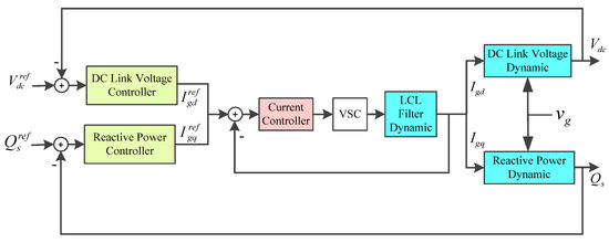
Figure 2.
Double loop control structure of the grid-connected inverter.
3.1. Output Current Control
Modeling of a three-phase grid-connected inverter with an LCL filter in dq frame results in a 2-inputs-2-outputs transfer function from inverter terminal voltages to grid-side currents, as given in (16),
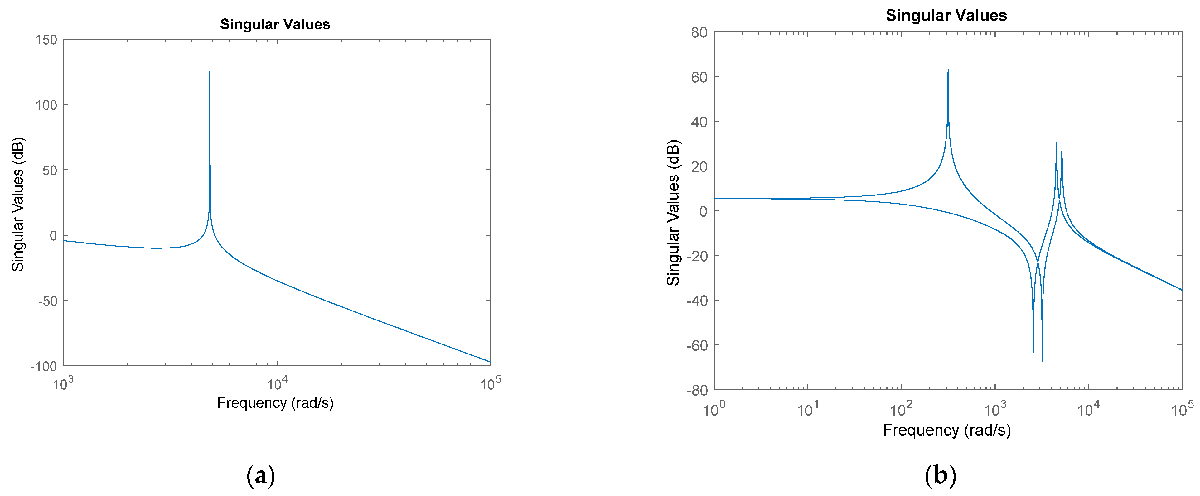
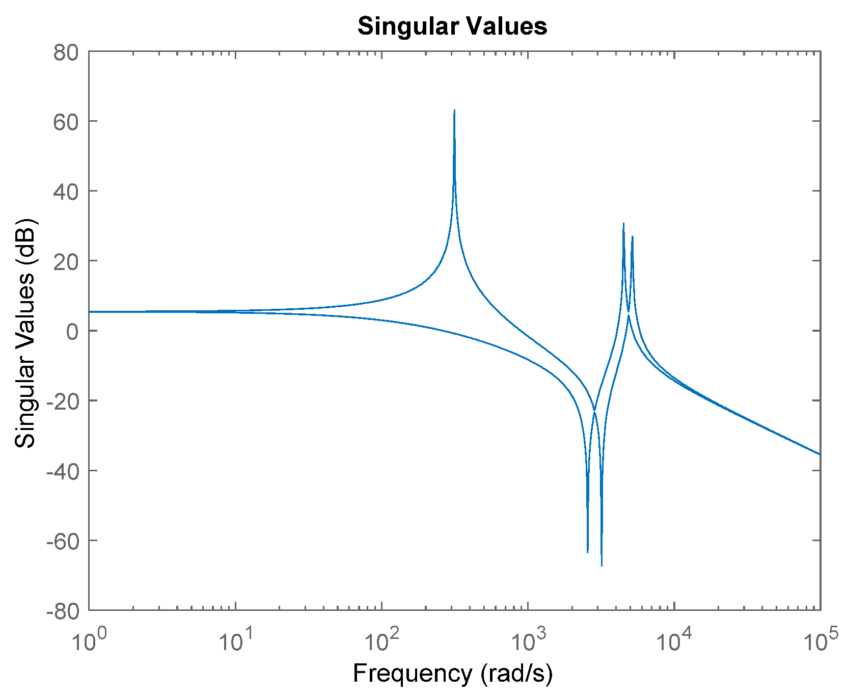
in which (, ) are the control inputs, (, ) are outputs, and the G matrix is the non-diagonal transfer function. Meanwhile, modeling of the system in an ABC frame results in a single input-single output transfer function for each phase of the system. In this regard, the frequency characteristics of a single LCL filter and the system in (16) are different, as shown in Figure 3. The resonance mode of the system is evident in both frequency characteristics.
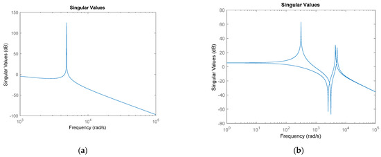
Figure 3.
Frequency characteristics of (a) single phase LCL filter and (b) the system in dq frame (transfer function in (16)).
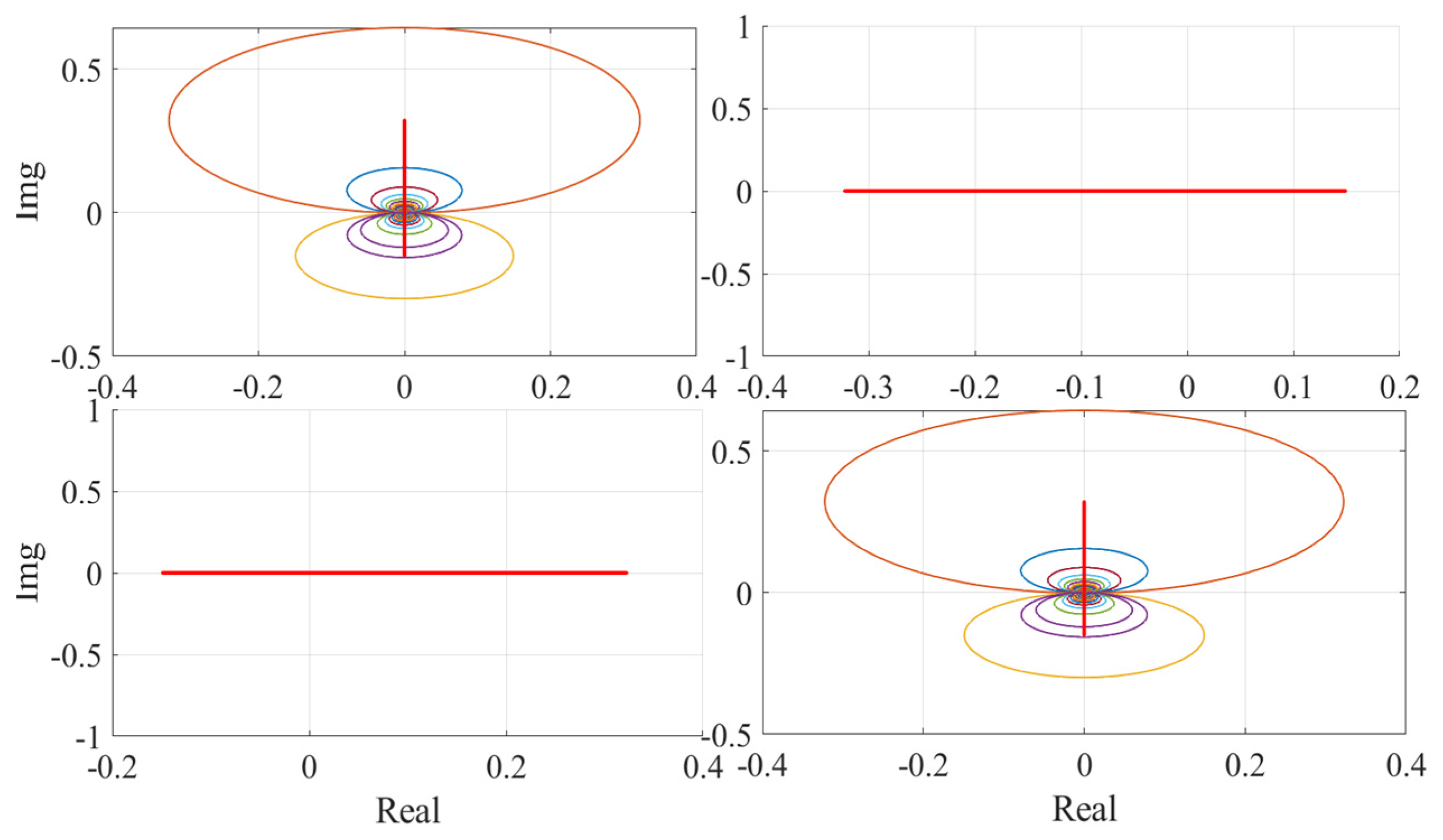
Considering the transfer function in (16), there is a tight coupling between two channels (channel 1: input 1 to output 1, channel 2: input 2 to output). Figure 4 shows the Gershgorin band graph of (16) with the parameter values of Table 2, which shows that the system is not column and row dominant. Also, based on the MIMO control system theory, the independent control design for channel 1 and channel 2 may lead to instability of the overall system, regardless of the resonance mode being dampened [29]. The high order of the system and the existence of the resonance mode are other factors that increase the difficulty of the current controller design.

Figure 4.
Gershgorin band graph of transfer function (16) with the parameter values of Table 3.
Table 2.
Effect of the control parameter on PM and bandwidth of the current control loop.
Based on the multivariable control theory, it is possible to decrease the coupling between channels in MIMO systems using a pre-controller such that the system becomes dominantly diagonal (column dominant or row dominant). However, it is not possible to completely remove the coupling and make the system diagonal using the mentioned pre-controller. To remove the coupling terms completely, a non-linear control scheme is proposed in this paper, which simultaneously damps the resonance modes. This controller is based on the back-stepping method, which is categorized as a state-feedback approach. To start the controller design with this method, two variables are defined as and , and an error variable vector is also defined as given by (17):
where,
The reference vector values are given in (19) which are obtained by solving the state Equations (6)–(11) in a steady state. Also, and are obtained by the reactive power and the DC-link voltage control loops, respectively.
According to the above definitions, the error state equations of the system are as given by (20)–(25).
The proposed controller drives and to zero, independently, which indicates that and are forced to their reference values with no coupling and interaction. The details of the proposed scheme are provided in the following subsections.
3.1.1. Proposed Active Current Control
To drive , as an active current, into , has to be forced to zero through proper selection of control variables. To do so, the term is added or subtracted to or from the right-hand side of in (24), as shown in (26).
By defining the new variable of as (27), (26) is rewritten as (28)
The derivative of is named in the rest of the paper, as given in (29).
Substituting and from (24)–(25) into (29), and defining the intermediate variable of , (29) is rewritten as:
If is enforced to zero, based on (28), will be equal to ; and then, for a positive value of , will go to zero exponentially. To do so, the positive definite Lyapunov function is defined as follows:
The derivative of (31) is given in (32).
Substituting (28) and (30) into (32) results in (33).
Based on (33), if is forced to (34), (33) is derived to (35).
Accordingly, selecting the positive values for and guarantees the force of and to zero based on the Lyapunov stability theorem [34].
Now, in (34) is added and subtracted to the right-hand side of (30) as:
Now, the new variable of is defined as given in (37).
Using the expression of from (37), (36) changes to (38).
The derivative of is also as given in (39).
From the above discussions, it is concluded that in order to drive to zero, and should also move to zero. For this purpose, another positive definite Lyapunov function is defined as shown in (40).
The derivative of the Lyapunov function with respect to the time is as given in (41).
substituting and respectively from (28) and (38), (41) is changed to (42).
Therefore, if is equal to , then, based on (39), is achieved by selecting as (43)
Equation (42) is equal to (44)
Therefore, according to (44) and based on the Lyapunov theorem, all variables of , , and move exponentially to zero. Deriving to zero exponentially indicates the independent tracking of the reference value of from other variables, especially without any interaction with the reactive current dynamics. The resonance modes are also dampened. Moreover, the poles of the control system, related to the active current control channel, are equal to , , and , which are the control parameters in (43). The poles are pure real with zero imaginary part which indicates complete damping of resonance mode.
Finally, the input control variable is as given in (45).
in which, can be further simplified from (43) to (46).
where,
3.1.2. Proposed Reactive Current Control
The method for control of is similar to that of , with a difference that the process begins with Equation of in (20) and (25). For the sake of brevity, the details of the controller design process are not elaborated here. By performing a similar procedure for , the final input control variable is as given by (53).
where,
in which, the coefficients are as given in the following equations of (55)–(60).
Using the control input of in (53) leads to the derivative of the new defined positive definite function of (61)
As follows,
where,
Based on the Lyapunov theorem and considering (61) and (62), all variables of , , and move exponentially to zero. Deriving to zero exponentially means the independent tracking of the reference value of from other variables, especially without any interaction with the active current dynamics. Also, the resonance mode is dampened properly.
Moreover, the poles of the control system, related to reactive current control channel, are equal to , , and which are the control parameters in (54) and (55). The poles are pure real with zero imaginary part which means complete damping of the resonance mode.
3.2. DC-Link Voltage Controller
As the DC-link voltage control is not the concern of this paper, the conventional DC-link voltage control scheme is presented in this subsection for the ease of reference. As shown in (13), both and affect the dynamics of the DC-link voltage. To remove the dynamic dependency to , it is a commonly used strategy to add as a feed-forward to the control system [32]. Thus, is the variable which is solely used for control of DC-link energy. Equation (65) represents the proper reference value of ,
where, (; ) are proportional and integral gains of the PI controller, respectively.
Using the reference value of in (65), the closed loop transfer function of the DC-link energy loop is as given by (66).
With reference to (66), the fast step response, high system bandwidth, zero steady state error, and proper robustness in presence of uncertainties in the system parameters are achieved by a proper setting of (; ) values.
3.3. Reactive Power Controllers
As the reactive power control is not the concern of this paper, the conventional reactive power control scheme is presented in the subsection for the ease of reference. To control reactive power, is the control operator. Equation (67) gives the proper current reference for control of reactive power associated with the reactive power reference value ().
where, is defined as given in (68).
Accordingly, tends to zero; and therefore, becomes equal to . The first term in right hand side of (67) is a feed-forward controller to speed up the tracking of the reactive power reference.
3.4. Proposed Observer for Estimation of State Variables of the LCL Filter
To obtain proper performance using the active damping methods, it is necessary to feedback all the state variables of the LCL filter such as the proposed controller in (45) and (53). This requirement demands the sensors for measuring all state variables, which is not cost effective. However, the need of the mentioned sensors is effectively resolved by using state variable estimation methods. Namely, measuring the grid current ( makes the overall system observable, and the filter capacitor voltage and the inverter current can be effectively estimated. Analysis of the state equations of a single phase LCL filter in static frame, given by (69), shows that measuring makes the system fully observable.
Accordingly, is measured directly and using a reduced-order Luenberger (ROL) observer, and are estimated. A second-order observer for estimation of and of each phase is utilized in this paper. Details of the Luenberger observer design procedure can be found in [35], which is not elaborated for the sake of brevity. According to the observer design procedure, the bandwidth of the observer should be selected higher than that of the main closed loop-controlled system.
Based on the discussions presented in the above subsections, the complete block diagram of the proposed controller is as depicted in Figure 5.
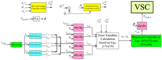
Figure 5.
Block diagram of the proposed controller.
4. Proposed Procedure for Tuning the Proposed Controller
According to (44) and (62), an increase of the controller parameters values ( and ) increases the bandwidth of the current control loop. However, due to the time delay imposed by computations and PWM sampling in the current control loop, the loop PM and the stability are affected. Therefore, the controller parameters should be selected carefully to obtain the desired stability margin and bandwidth.
4.1. Proposed Scheme for Phase Margin Determination
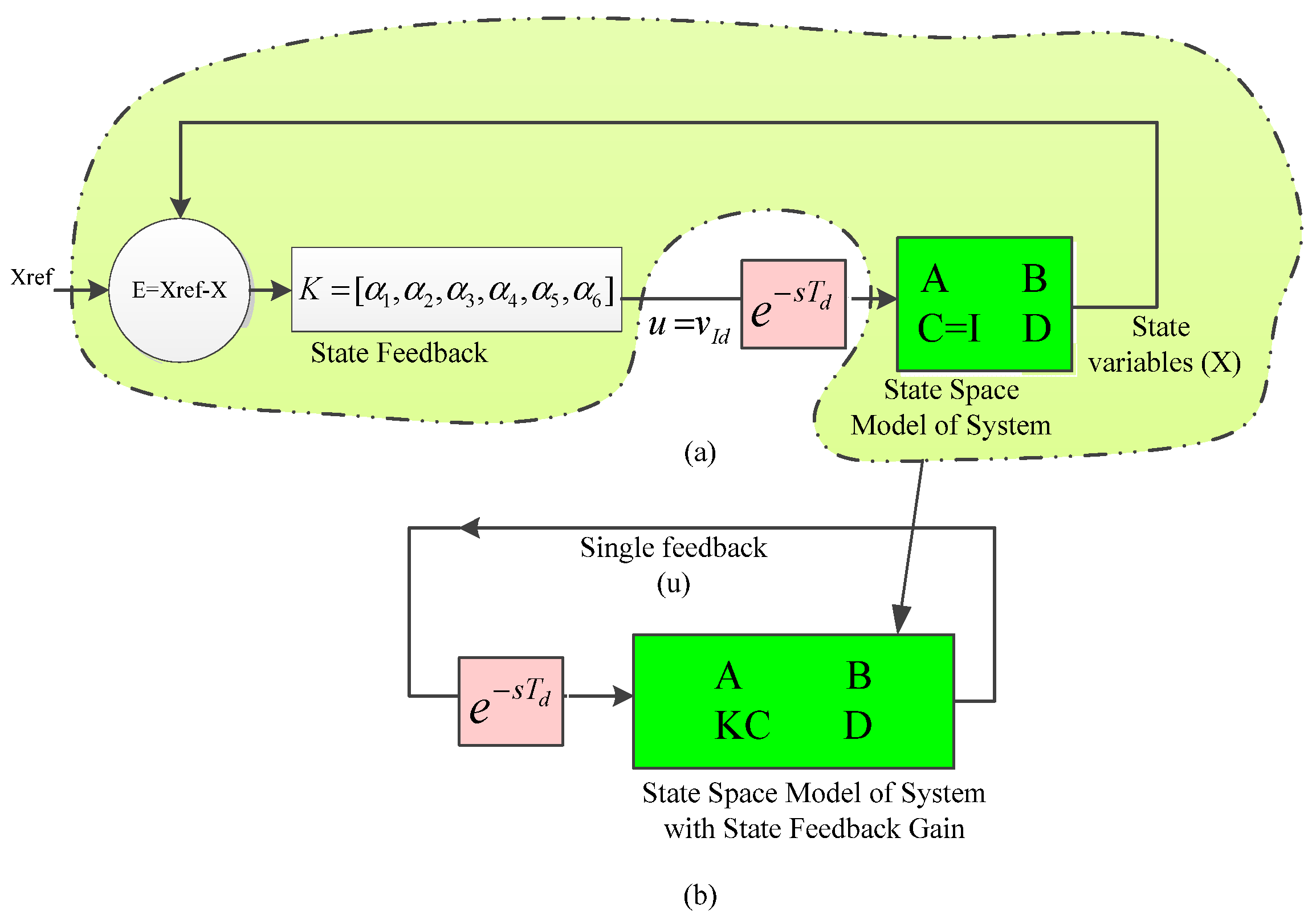
It was shown previously that the control structure of a grid-connected VSC with an LCL type filter in the dq frame is a MIMO system. In order to evaluate the stability margin of the system, PM and the gain margin are required. However, the PM concept is used for SISO systems, and there is no accurate and straightforward mechanism to determine the PM of a non-SISO system. In this subsection, a proposed scheme for PM determination is presented, which uses the advantage of decoupling the control channels of and channels in the proposed control scheme.
The proposed controller of Figure 5 is a type of state feedback controller, and Figure 6a shows its simplified diagram for control of channel. Therefore, the well-known PM determination method used for the SISO system cannot be applied here. However, if the gain matrix of state feedback () is combined with system state space equations, the single signal can be considered as feedback signal. Thus, the new system will be a SISO system, and the PM of the system can be evaluated accordingly.
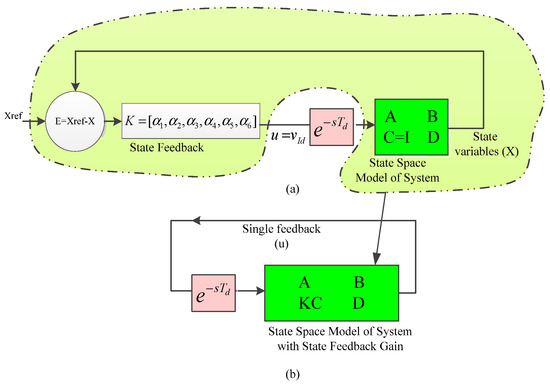
Figure 6.
Converting a state feedback loop (a) to a single output feedback loop (b).
4.2. Proposed Approach for Controller Parameters Tuning
Using the proposed method, the PM and tolerable time delay in current control loop () are determined for the studied system of Table 2. For the sake of simplicity, the values of all control parameters are considered the same () and PM, , and bandwidth of the and control loops are determined for the different values of the control parameter . It can be observed that an increase in control parameter decreases and increases the bandwidth (). The total time delay in the control loop due to computations and PWM sampling is . Indeed, the control parameter should be selected such that is greater than .
Considering and (according to system parameters in Table 3), the total time delay in the current control loop is . Therefore, the controller parameter is selected as , which results in , considering in the control loop, and current loop bandwidth . Accordingly, the PI controller parameters for the DC-link voltage and the reactive power controller are selected as , and . Using the selected , and , PM of the DC-link voltage and the reactive power control loops are about and respectively. Also, the DC-link voltage and the reactive power control loop bandwidths are selected at , which is about five times lower than that of the current control loop.
Table 3.
The test system parameters.
5. Case Study and Simulation Results
To verify the performance of the proposed control scheme, at first, the frequency characteristic of the closed loop system is shown in Figure 7. In comparison with the frequency characteristic of an open loop system in Figure 3b, it is evident that the resonance mode of the controlled system has been damped completely. Furthermore, different simulation case studies are provided in this section. The switching frequency and the sampling rate both are 10 kHz, and the computational time in each sample is considered 100 µs in a simulated system. The parameter values of the system and controllers are presented in Table 3.
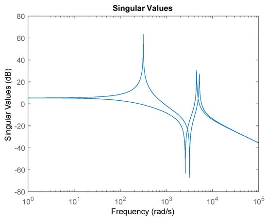
Figure 7.
Frequency characteristics of the closed loop system.
In this section, three cases are studied: (i) the converter is connected to an ideal grid with zero impedance, without any uncertainty in the system parameters, (ii) the converter is connected to the grid through non-zero impedance, and (iii) the grid impedance is non-zero, and there is uncertainty in the parameters of the system.
In the following, the description of the operating condition in the scenarios are provided. At first, is 30 kW, is 10 kVAr, and the desired DC-link voltage is 1000 V. To show the dynamic results, the following changes are applied to the operating point.
- 1.
- at t = 0.1 s, steps up to 20 kVar;
- 2.
- at t = 0.2 s, steps up to 25 kW;
- 3.
- at t = 0.3 s, steps up to 1050 V;
- 4.
- at t = 0.4 s, steps down to 1000 V.
5.1. Converter Is Connected to an Ideal Grid (Zero Impedance)
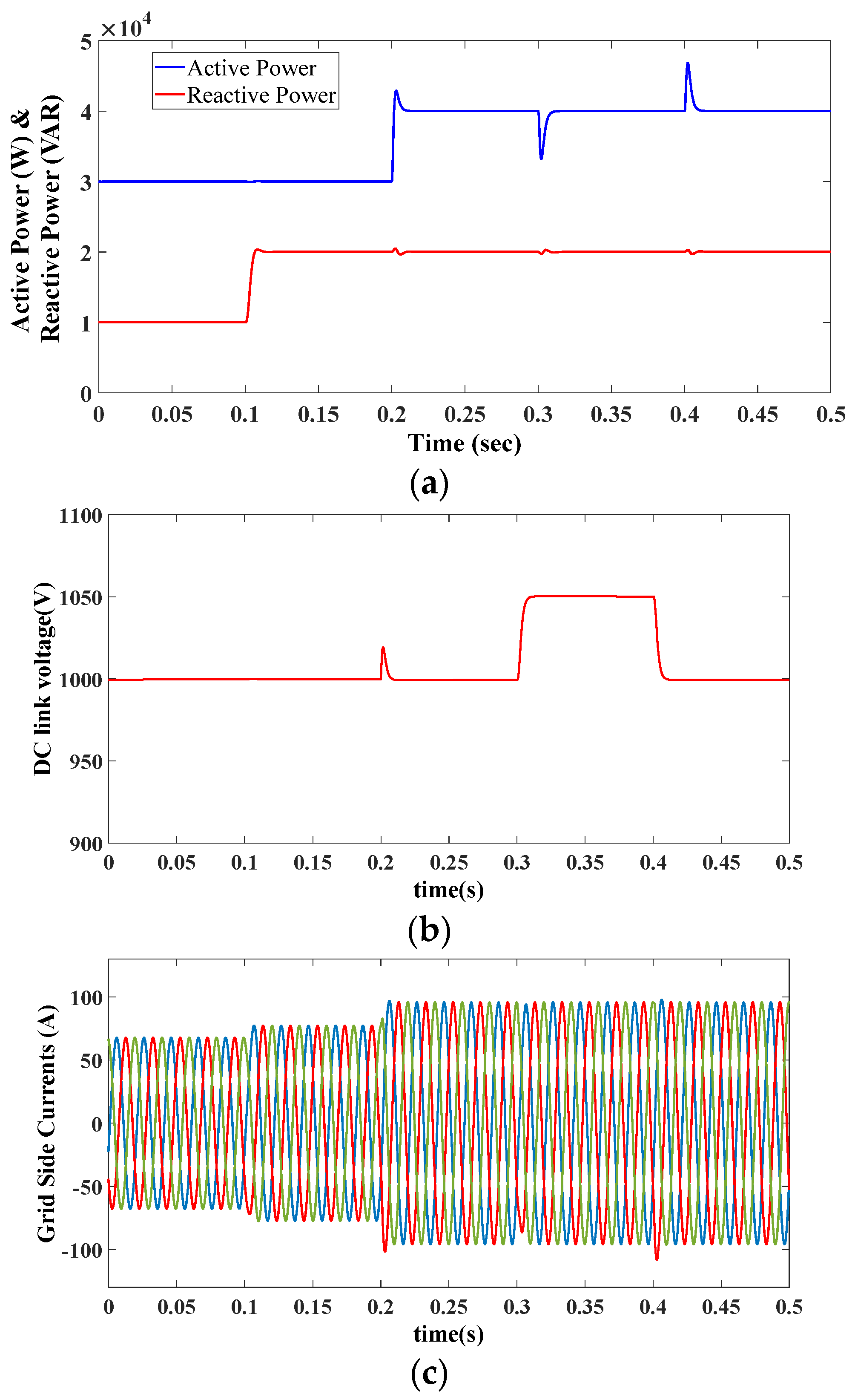
In this case, the grid Thevenin impedance is considered negligible (). The results of the simulation are presented in Figure 8, indicating that both the DC-link voltage and the reactive power smoothly track their reference values. Also, the changes of and have a negligible effect on each other. This confirms that the coupling between the active and reactive power channels is effectively removed. The minor coupling observed in the simulation results of Figure 8 is due to the time delay and observer operation in the control loop.
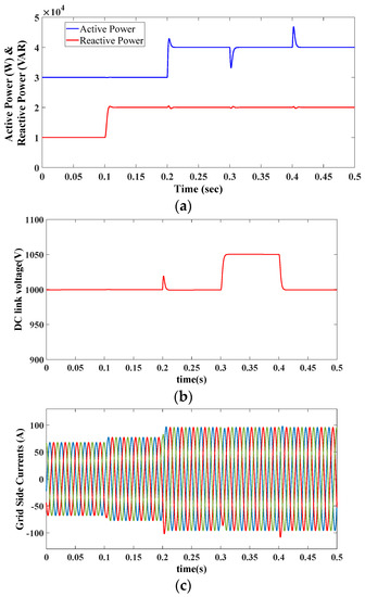
Figure 8.
The response of the system connected to a zero-impedance grid; (a) the active and the reactive power, (b) the DC-link voltage, and (c) grid-side currents.
5.2. Converter Is connected to a Non-Ideal Grid (Non-Zero Impedance)
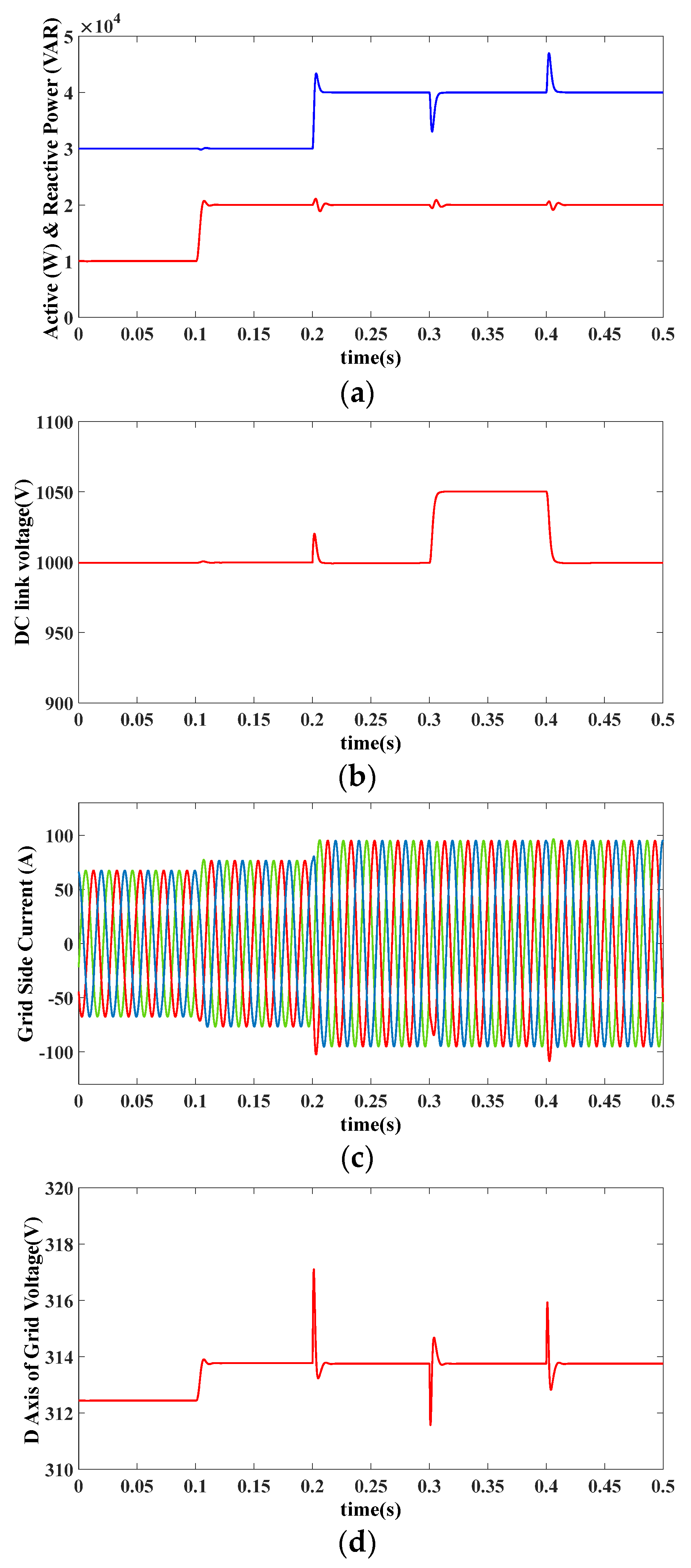
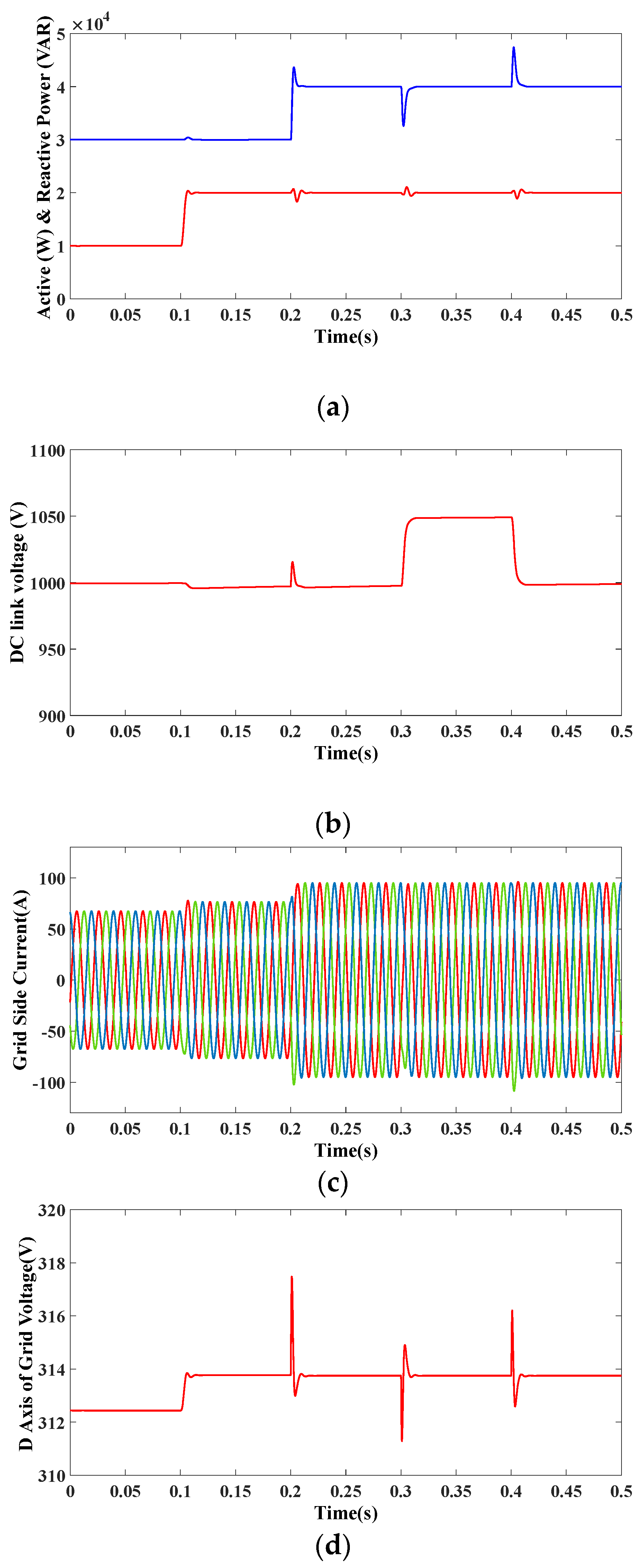
In this part, the converter is connected to a non-ideal grid with which corresponds to . Accordingly, the resonance frequency of the system is changed to 662 Hz. The scenarios and the applied reference commands are the same to those of the previous sub-section. The simulation results are presented in Figure 9. As expected, the non-zero grid impedance has a negligible effect on the performance of the proposed control scheme. According to the results, the fast response, the high stability margin of the system, with negligible coupling between the active and reactive power channels, are achieved by using the proposed control scheme. As shown in Figure 9c, the changes of the active and reactive power affect the grid voltage, which consequently results in a small coupling (slightly more than the previous cases).
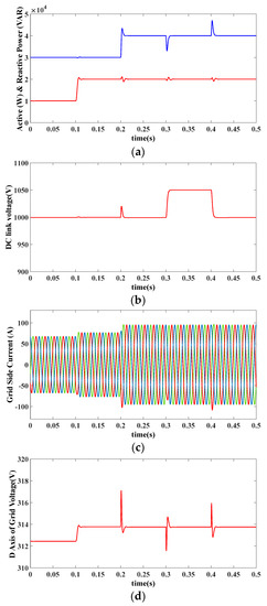
Figure 9.
Response of the simulated system with ; (a) the active and the reactive powers, (b) the DC-link voltage, (c) grid-side currents, and (d) PCC voltage magnitude.
5.3. Converter Is Connected to a Non-Ideal Grid (Non-Zero Impedance) Considering Uncertainties in the Filter Impedances
In this subsection, the robustness of the proposed controller in the presence of uncertainties in the system parameters is evaluated. It is supposed that there is 20% uncertainty in the filter inductances, i.e., their values are and , whereas the controller is designed for and . The grid inductance is also considered . The simulation results are presented in Figure 10. The fast and proper dynamic response of the system are concluded from the results. Similar to the previous subsections, there is a negligible interaction between the active and the reactive power control channels (slightly more than the previous cases) due to the time delay, observer operation, grid impedance, and uncertainty in the control loop.
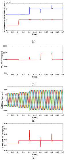
Figure 10.
Response of the simulated system with , , and ; (a) the active and the reactive powers, (b) the DC-link voltage, (c) grid-side currents, and (d) PCC voltage magnitude.
6. Conclusions
This paper has presented a nonlinear control scheme for decoupling the output active and reactive current controls of a grid-connected VSC with LCL type filters and damping its resonance mode. The system is an LTI-MIMO system with two-inputs-two-outputs in the dq frame. The system has a resonance mode, and there is a solid coupling between the active and reactive current channels. The proposed controller decouples the channels and damps the resonance mode of the LCL filter effectively. Also, a simple scheme was presented to determine the PM of the current control loops. Then, using the presented PM determination method and considering the time delay in the control loop, parameters of the controller are tuned to reach the proper bandwidth and stability margin. To minimize the number of sensors, an ROL observer is employed in which only the grid current was measured directly and the other state variables of the LCL filter were estimated. The performance of the proposed controller in different perspectives was demonstrated through various simulations.
Author Contributions
M.A.G. and S.F.Z. wore the paper. M.A.G. provided the idea and simulated the hypothesis. S.F.Z. analyzed the results and helped the simulation of the main idea. S.P. and F.B. discussed the results and edited the paper. All authors have read and agreed to the published version of the manuscript.
Funding
This research received no external funding.
Institutional Review Board Statement
Not applicable.
Informed Consent Statement
Not applicable.
Data Availability Statement
Not applicable.
Conflicts of Interest
The authors declare no conflict of interest.
References
- Zarei, S.F.; Ghasemi, M.A.; Mokhtari, H.; Blaabjerg, F. Performance Improvement of AC-DC Power Converters under Un-balanced Conditions. Scientia Iranica 2019. [Google Scholar] [CrossRef] [Green Version]
- Beres, R.N.; Wang, X.; Liserre, M.; Blaabjerg, F.; Bak, C.L. A Review of Passive Power Filters for Three-Phase Grid-Connected Voltage-Source Converters. IEEE J. Emerg. Sel. Top. Power Electron. 2016, 4, 54–69. [Google Scholar] [CrossRef] [Green Version]
- Sanatkar-Chayjani, M.; Monfared, M. Stability Analysis and Robust Design of LCL With Multituned Traps Filter for Grid-Connected Converters. IEEE Trans. Ind. Electron. 2016, 63, 6823–6834. [Google Scholar] [CrossRef]
- Khajehoddin, S.A.; Karimi-Ghartemani, M.; Jain, P.K.; Bakhshai, A. A Control Design Approach for Three-Phase Grid-Connected Renewable Energy Resources. IEEE Trans. Sustain. Energy 2011, 2, 423–432. [Google Scholar] [CrossRef]
- Xu, J.; Xie, S. LCL-resonance damping strategies for grid-connected inverters with LCL filters: A comprehensive review. J. Mod. Power Syst. Clean Energy 2017, 6, 292–305. [Google Scholar] [CrossRef] [Green Version]
- Yao, W.; Yang, Y.; Zhang, X.; Blaabjerg, F.; Loh, P.C. Design and Analysis of Robust Active Damping for LCL Filters Using Digital Notch Filters. IEEE Trans. Power Electron. 2017, 32, 2360–2375. [Google Scholar] [CrossRef] [Green Version]
- Pena-Alzola, R.; Liserre, M.; Blaabjerg, F.; Ordonez, M.; Kerekes, T. A Self-commissioning Notch Filter for Active Damping in a Three-Phase LCL -Filter-Based Grid-Tie Converter. IEEE Trans. Power Electron. 2014, 29, 6754–6761. [Google Scholar] [CrossRef] [Green Version]
- Ciobotaru, M.; Rossé, A.; Bede, L.; Karanayil, B.; Agelidis, V.G. Adaptive Notch filter based active damping for power con-verters using LCL filters. In Proceedings of the 7th International Symposium on Power Electronics for Distributed Generation Systems (PEDG), Vancouver, BC, Canada, 27–30 June 2016; pp. 1–7. [Google Scholar]
- Mahlooji, M.H.; Mohammadi, H.R.; Rahimi, M. A review on modeling and control of grid-connected photovoltaic inverters with LCL filter. Renew. Sustain. Energy Rev. 2018, 81, 563–578. [Google Scholar] [CrossRef]
- Midtsund, T. Control of Power Electronic Converters in Distributed Power Generation Systems: Evaluation of Current Control Structures for Voltage Source Converters operating under Weak Grid Conditions. In Proceedings of the 2nd International Symposium on Power Elec-tronics for Distributed Generation Systems, Hefei, China, 16–18 June 2010; pp. 382–388. [Google Scholar]
- Bao, C.; Ruan, X.; Wang, X.; Li, W.; Pan, D.; Weng, K. Step-by-Step Controller Design for LCL-Type Grid-Connected Inverter with Capacitor–Current-Feedback Active-Damping. IEEE Trans. Power Electron. 2014, 29, 1239–1253. [Google Scholar] [CrossRef]
- Pan, D.; Ruan, X.; Bao, C.; Li, W.; Wang, X. Capacitor-Current-Feedback Active Damping With Reduced Computation Delay for Improving Robustness of LCL-Type Grid-Connected Inverter. IEEE Trans. Power Electron. 2014, 29, 3414–3427. [Google Scholar] [CrossRef]
- Xia, W.; Kang, J. Stability of LCL-filtered grid-connected inverters with capacitor current feedback active damping considering controller time delays. J. Mod. Power Syst. Clean Energy 2017, 5, 584–598. [Google Scholar] [CrossRef] [Green Version]
- Komurcugil, H.; Altin, N.; Ozdemir, S.; Sefa, I. Lyapunov-Function and Proportional-Resonant-Based Control Strategy for Single-Phase Grid-Connected VSI With LCL Filter. IEEE Trans. Ind. Electron. 2016, 63, 2838–2849. [Google Scholar] [CrossRef]
- Xu, A.J.; Xie, B.S.; Kan, C.J.; Ji, D.L. An improved inverter-side current feedback control for grid-connected inverters with LCL filters. In Proceedings of the 2015 9th International Conference on Power Electronics and ECCE Asia (ICPE-ECCE Asia), Seoul, Korea, 1–5 June 2015; pp. 984–989. [Google Scholar]
- Judewicz, M.G.; Gonzalez, S.A.; Fischer, J.R.; Martinez, J.F.; Carrica, D.O. Inverter-Side Current Control of Grid-Connected Voltage Source Inverters WITH LCL Filter Based on Generalized Predictive Control. IEEE J. Emerg. Sel. Top. Power Electron. 2018, 6, 1732–1743. [Google Scholar] [CrossRef] [Green Version]
- Maccari, L.A.; Massing, J.R.; Schuch, L.; Rech, C.; Pinheiro, H.; Oliveira, R.; Montagner, V.F. LMI-Based Control for Grid-Connected Converters With LCL Filters Under Uncertain Parameters. IEEE Trans. Power Electron. 2014, 29, 3776–3785. [Google Scholar] [CrossRef]
- Hao, X.; Yang, X.; Liu, T.; Huang, L.; Chen, W. A Sliding-Mode Controller With Multiresonant Sliding Surface for Single-Phase Grid-Connected VSI With an LCL Filter. IEEE Trans. Power Electron. 2012, 28, 2259–2268. [Google Scholar] [CrossRef]
- Nϕrgaard, J.B.; Graungaard, M.K.; Dragičević, T.; Blaabjerg, F. Current Control of LCL-Filtered Grid-Connected VSC Using Model Predictive Control with Inherent Damping. In Proceedings of the 20th European Conference on Power Electronics and Applications (EPE’18 ECCE Europe), Riga, Latvia, 17–21 September 2018; pp. P.1–P.9. [Google Scholar]
- Zhang, X.; Wang, Y.; Yu, C.; Guo, L.; Cao, R. Hysteresis Model Predictive Control for High-Power Grid-Connected Inverters With Output LCL Filter. IEEE Trans. Ind. Electron. 2016, 63, 246–256. [Google Scholar] [CrossRef]
- Karamanakos, P.; Nahalparvari, M.; Geyer, T. Fixed Switching Frequency Direct Model Predictive Control with Continuous and Discontinuous Modulation for Grid-Tied Converters With LCL Filters. IEEE Trans. Control. Syst. Technol. 2020, 29, 1503–1518. [Google Scholar] [CrossRef]
- Nam, N.N.N.; Nguyen, N.-D.; Yoon, C.; Choi, M.; Lee, Y.I. Voltage Sensorless Model Predictive Control for a Grid-Connected Inverter with LCL Filter. IEEE Trans. Ind. Electron. 2021. [Google Scholar] [CrossRef]
- Shuitao, Y.; Qin, L.; Peng, F.Z.; Zhaoming, Q. A Robust Control Scheme for Grid-Connected Voltage-Source Inverters. IEEE Trans. Ind. Electron. 2011, 58, 202–212. [Google Scholar]
- Gabe, I.J.; Montagner, V.F.; Pinheiro, H. Design and Implementation of a Robust Current Controller for VSI Connected to the Grid Through an LCL Filter. IEEE Trans. Power Electron. 2009, 24, 1444–1452. [Google Scholar] [CrossRef]
- Chowdhury, V.R.; Kimball, J.W. Robust Control Scheme for a Three Phase Grid-Tied Inverter With LCL Filter During Sensor Failures. IEEE Trans. Ind. Electron. 2020, 68, 8253–8264. [Google Scholar] [CrossRef]
- Qingrong, Z.; Liuchen, C. An Advanced SVPWM-Based Predictive Current Controller for Three-Phase Inverters in Distributed Generation Systems. IEEE Trans. Ind. Electron. 2008, 55, 1235–1246. [Google Scholar] [CrossRef]
- Massing, J.R.; Stefanello, M.; Grundling, H.A.; Pinheiro, H. Adaptive Current Control for Grid-Connected Converters With LCL Filter. IEEE Trans. Ind. Electron 2012, 59, 4681–4693. [Google Scholar] [CrossRef]
- Espi, J.M.; Castello, J.; Garcia-Gil, R.; Garcera, G.; Figueres, E. An Adaptive Robust Predictive Current Control for Three-Phase Grid-Connected Inverters. IEEE Trans. Ind. Electron. 2010, 58, 3537–3546. [Google Scholar] [CrossRef] [Green Version]
- Skogestad, S.; Postlethwaite, I. Multivariable Feedback Control: Analysis and Design; John Wiley & Sons: Hoboken, NJ, USA, 2005. [Google Scholar]
- Ghasemi, M.A.; Parniani, M.; Zarei, S.F.; Foroushani, H.M. Fast maximum power point tracking for PV arrays under partial shaded conditions. In Proceedings of the 18th European Conference on Power Electronics and Applications (EPE’16 ECCE Europe), Karlsruhe, Germany, 5–8 September 2016; pp. 1–12. [Google Scholar]
- Zarei, S.F.; Mokhtari, H.; Ghasemi, M.A. Enhanced control of grid forming VSCs in a micro-grid system under unbalanced conditions. In Proceedings of the 2018 9th Annual Power Electronics, Drives Systems and Technologies Conference (PEDSTC), Tehran, Iran, 13–15 February 2018; pp. 380–385. [Google Scholar]
- Ghoddami, H.; Yazdani, A. A Single-Stage Three-Phase Photovoltaic System With Enhanced Maximum Power Point Tracking Capability and Increased Power Rating. IEEE Trans. Power Deliv. 2010, 26, 1017–1029. [Google Scholar] [CrossRef]
- Zarei, S.; Mokhtari, H.; Ghasemi, M.; Peyghami, S.; Davari, P.; Blaabjerg, F. DC-link loop bandwidth selection strategy for grid-connected inverters considering power quality requirements. Int. J. Electr. Power Energy Syst. 2020, 119, 105879. [Google Scholar] [CrossRef]
- Khalil, H.K.; Grizzle, J. Nonlinear Systems; Prentice Hall: Hoboken, NJ, USA, 1996; Volume 3. [Google Scholar]
- Luenberger, D. An introduction to observers. IEEE Trans. Autom. Control. 1971, 16, 596–602. [Google Scholar] [CrossRef]


Publisher’s Note: MDPI stays neutral with regard to jurisdictional claims in published maps and institutional affiliations. |
© 2021 by the authors. Licensee MDPI, Basel, Switzerland. This article is an open access article distributed under the terms and conditions of the Creative Commons Attribution (CC BY) license (https://creativecommons.org/licenses/by/4.0/).