Article

Compliance of Distribution System Reactive Flows with Transmission System Requirements

by
Panagiotis Pediaditis
1,*,
Katja Sirviö
2,
Charalampos Ziras
3,
Kimmo Kauhaniemi
2,
Hannu Laaksonen
2 and
Nikos Hatziargyriou
1
1
School of Electrical and Computer Engineering, National Technical University of Athens, 15780 Zografou, Greece
2
School of Technology and Innovations, University of Vaasa, 65100 Vaasa, Finland
3
Department of Electrical Engineering, Technical University of Denmark, 2800 Kgs. Lyngby, Denmark
*
Author to whom correspondence should be addressed.
Appl. Sci. 2021, 11(16), 7719; https://doi.org/10.3390/app11167719
Submission received: 18 June 2021 / Revised: 10 August 2021 / Accepted: 16 August 2021 / Published: 22 August 2021

Abstract

:
Transmission system operators (TSOs) often set requirements to distribution system operators (DSOs) regarding the exchange of reactive power on the interface between the two parts of the system they operate, typically High Voltage and Medium Voltage. The presence of increasing amounts of Distributed Energy Resources (DERs) at the distribution networks complicates the problem, but provides control opportunities in order to keep the exchange within the prescribed limits. Typical DER control methods, such as constant cos ϕ or Q/V functions, cannot adequately address these limits, while power electronics interfaced DERs provide to DSOs reactive power control capabilities for complying more effectively with TSO requirements. This paper proposes an optimisation method to provide power set-points to DERs in order to control the hourly reactive power exchanges with the transmission network. The method is tested via simulations using real data from the distribution substation at the Sundom Smart Grid, in Finland, using the operating guidelines imposed by the Finnish TSO. Results show the advantages of the proposed method compared to traditional methods for reactive power compensation from DERs. The application of more advanced Model Predictive Control techniques is further explored.

1. Introduction

1.1. Background and Motivation

Distributed Energy Resources (DERs) in Active Distribution Networks (ADNs) create challenges for the Transmission System Operators (TSOs) and the Distribution System Operators (DSOs) but also provide opportunities to improve network operation and services [1]. In the future, active and reactive power flows between Distribution Networks (DNs) and Transmission Networks (TNs) can change more rapidly due to the intermittent nature of renewable generation and higher load uncertainty. Therefore, more active and shorter-term control of reactive power flow between these networks is needed to minimise voltage fluctuations and losses at the TN level. DER units with inverter-based interfaces are potential flexibility resources capable of providing services without additional investments in new network assets/components next to traditional voltage control and congestion management related services.
In the context of TSO/DSO collaboration, it can be stated that ADNs are desired to provide local (up to the DSO level) and system-wide (up to the TSO level) ancillary services (AS) through DERs. One local AS is reactive power control through DER units for satisfying the TSO’s requirements for reactive power flow exchange. In some practical cases, excessive reactive power flows are penalised by TSOs, thus it is beneficial to find an optimal way to control DER reactive power support.

1.2. Literature Review

Several works have investigated the topic of reactive power exchange between transmission and distribution grids in the past. In [2,3], novel methods are presented for assessing the range of controllable reactive power available at the transmission node for any level of active power exchange with the distribution network. In [4], particle swarm optimisation is used to exploit wind farm active and reactive power control capability to achieve a reactive power exchange level. In [5], the objectives of maintaining safe voltage levels and respecting the reactive power exchange limits in distribution networks are achieved via a ruled-based method and the use of an iterative process. In [6], Model Predictive Control (MPC) is employed for achieving multiple objectives, among which is the minimisation of reactive power exchange, and in [7] the method is expanded to include the potential for DSOs to provide a range of reactive power set-points as a service to the TSO, according to DN capabilities. In [8], a rule-based central controller is calculating the reactive power compensation level from Distributed Generators (DG), to which level the DG comply according to their capabilities. In [9], a two-stage optimisation method is employed for controlling both voltage levels and reactive power exchange. The tap positions of capacitor banks are optimised on a daily basis, and reactive power support from DG on an hourly basis.
Overall, the proposed methodologies can be divided into those that have as an objective to minimise deviations from set-points [4,6,7] and those that have as a constraint to keep the reactive power exchange within certain limits [5,8,9]. This paper falls in the second category, and its objective is to keep reactive power exchange between transmission and distribution grids within the limits specified by the TSO. Specifically, the limits of the Finish TSO, Fingrid [10]. The recent requirements of the Finnish TSO do not define a simple static upper and lower limit for reactive power exchange, but a complex structure that depends on active power exchange.
Previous attempts to solve this problem have been made in the past. Different requirements for the reactive power flow at the TN and DN Point of Interconnection (POI), for the Finnish distribution grid case, and tested at the Sundom Smart Grid, is presented in [11]. This paper considers requirements for (1) European Commission’s conditions for reactive power management for the transmission grid-connected distribution systems [12], (2) the conditions set by Fingrid [13] and (3) the Non-Detection Zone (NDZ) requirements for microgrids [14,15,16]. It presents the “future reactive power window”—developed for the Sundom Smart Grid—and a reactive power controller for a 3.6 MW Wind Turbine (WT) unit connected to the MV bus with a full-scale converter that controls reactive power according to the Fingrid and NDZ requirements. Further, techno-economic case studies controlling the reactive power flow at the POI of the developing Sundom Smart Grid according to the Fingrid requirements are presented in [3]. The reactive power software controller development and implementation into the lightweight Intelligent Electronic Device (IED) microcontroller, based on IEC61850 GOOSE, and testing the IED in the real-time Controller Hardware-In-the-Loop (CHIL) platform are presented in [17,18]. The potential of accelerating the long-term simulation and CHIL testing is beneficial to the developing the DER controls for AS provision and is demonstrated in [19]. In all of these papers, the reactive power controllers were operating according to the last measurements of active and reactive power at the POI. Acceptable results were obtained by setting more tight reactive power limits than Fingrid requires. The work in [17] provides evidence for the need of developing a predictive controller.

1.3. Contribution and Organisation

This paper addresses the problem of adherence to the reactive power exchange limits between the distribution and transmission systems under cases of complex requirements, by utilising DER reactive power control capabilities. The case study of the Finnish TSO reactive power exchange requirements with the distribution network is taken as a real-life application. Expanding from the works in [11,14,15,16,17,18,19], this work proposes a novel method with the following features:
  • It introduces complex TSO requirements to a quadratically constrained quadratic programming optimisation problem that can be efficiently and timely solved.
  • It considers the constraints of the distribution system to ensure that DER compensation does not compromise network currents and voltages.
  • It cakes use of a short-term MPC framework that ensures control actions do not negatively affect the compliance with the requirement within the specified time frame set by the regulation.
The rest of the paper is organised as follows. In Section 2, the developed methodology is described, and in Section 3, the considered case studies are presented. Finally, Section 4 concludes the paper.

2. Problem Formulation

2.1. Problem Definition

According to the TSO requirement, reactive power flow Q via the primary DN substation (110 kV to 21 kV) should be confined within some specified limits, as shown in Figure 1. This limitation is applied to the hourly average reactive power exchange. This means that at the end of an hourly period the average reactive power through the root node of the DN ( Q ¯ 1 ), is constrained according to Figure 1. The upper and lower limits of Q ¯ 1 are a function of the corresponding average active power ( P ¯ 1 ). In case these limits are violated, the DSO is penalised.
The reactive power exchanged between the TN and the DN is affected by the reactive power consumed or produced by the loads, generating DERs, and the capacitance of the lines which is usually small in overhead lines, but significant in cables at low load. We assume that the DSO is allowed to control the reactive power absorbed/injected by DERs. Usually, grid codes mandate that DERs provide reactive power support, and this support does not entail additional costs to DSOs. Moreover, the DSO has to consider the physical constraints of the network, namely, line and voltage limits. We model the network using the LinDistFlow Equation [20].
The reactive power exchange requirements define an hourly time period for which the control goal is set. This period, lasting one hour, is called a control session and each day has 24 such sessions. Each of them is divided into a set, denoted by τ , of time steps indexed by τ . Thus, τ { 1 , , | | } or, equivalently, τ τ . In this study, there are 12 time steps in an hour. One control action is performed at every time step, i.e., one action every 5 min. The overall optimisation goal is to minimise the violation of the hourly average reactive power exchange limits, which are imposed by the TSO requirements of Figure 1 [10].
First, we outline the basic characteristics of the problem with the help of Equations (1)–(6). We further denote by q i , τ the decision variable which represents the DER reactive power support at node i and time step τ . A generic description of the overall problem is the following:
min q ( Q ¯ 1 limits violation )
network equations
Φ min ( P ¯ 1 ) Q ¯ 1 Φ max ( P ¯ 1 )
P ¯ 1 = 1 | T | τ T P 1 , τ
Q ¯ 1 = 1 | T | τ T Q 1 , τ
q i min q i , τ q i max , i I , τ T
where bold letters denote vectors. P 1 , τ and Q 1 , τ are the active and reactive power exchange through the root node of the DN, respectively. P ¯ 1 and Q ¯ 1 are their average values over the control session (here, an hour). Φ m i n and Φ m a x are functions of P ¯ 1 that define the limits on reactive power exchange and are dictated by Figure 1. Finally, q i m i n and q i m a x are the lower and upper limits of the reactive power support output of DER at node i.
Please note that model (1)–(6) serves as an aid for explaining key parts of the model and is not to be confused with the main model.The objective function of the problem is not discussed at this point, as it will be elaborated later in this section, but is based on a transformation of constraint (3). This constraint dictates that the average reactive power exchange via the root node is within the limits defined by Figure 1. This means that for a specific P ¯ 1 , there is a corresponding lower Φ min ( P ¯ 1 ) and upper Φ max ( P ¯ 1 ) limit of Q ¯ 1 .
The model in (1)–(6) is a deterministic multi-period optimisation problem. This means that if one was 100% certain about power injections P and Q all over the DN over the entire control session then the problem could be solved as it is formulated. However, these injections are stochastic parameters in reality. Control actions occur more often than the one hour control session (in this particular case every 5 min). This means that the problem can be solved every time step τ as a single period problem that considers the average power exchange until that time step only. Thus, the system has the opportunity to respond to new conditions that occurred within the duration of the control session, even without knowledge of the horizon. However, this approach is less efficient and, in some cases, might be insufficient in responding to sudden changes.
Elaborating more than solving the single-period problem on every time step τ , one can use a forecast of the system parameters for the remainder of the control session and solve the problem as a multi-period problem for the rest the control session. This setup is in practice an MPC formulation [21]. We will formulate our proposed model as an MPC model where its single-period equivalent is easily implied by the equations.
Some basic notation from MPC problems follows. There is an objective function, a horizon T, and a dynamic model of the system that is added to the problem constraints. On every time step τ , the problem is solved for the entire horizon, T τ , but we implement only the first control action u t = τ . At the next time step, τ + 1 , we repeat the process by solving the problem for horizon T τ + 1 and implement only the new first control action u t = τ + 1 .
There are two options regarding the horizon T τ at step τ . If it has fixed length, it is a receding horizon, meaning that it always ends at T steps away from τ . If the length is not fixed, but instead the end of the horizon is fixed, it is called shrinking horizon. In such a case, τ moves from 0 to T , and at every time step the optimisation horizon is T τ = T + 1 τ . In other words, the horizon is getting smaller and smaller as we move towards the end of the control session. In the problem of this paper, we have a shrinking horizon problem.

2.2. Model Formulation

The power flow equations of the distribution network are represented through the LinDistFlow model [20,22] which is a convex formulation. The set of distribution nodes is denoted by I + , while the subset I does not include the root node. As our network is radial, we can also denote the set of branches as I . We denote by j i the branch ending at node i. Finally, we denote by a i the parent node of node i and by K i the set of children nodes of node i. Figure 2 is used to describe the LinDistFlow model.
At every time step τ of the overall control session T , we have a new horizon T τ , where t T τ . Thus, the following optimisation problem is solved:
min q , Q ¯ 1 , Q , V J τ = objective function ( discussed in detail later in this section )
s . t : q i , t m i n q i , t q i , t m a x , i , t I , T τ
P i , t = P i , t L + k K i P i + k , t , i , t I , T τ
Q i , t = Q i , t L + q i , t + k K i Q i + k , t , i , t I , T τ
P i , t 2 + Q i , t 2 F ¯ i 2 , i , t I , T τ
V i , t = V i 1 , t 2 ( r i P i , t + x i Q i , t ) , i , t I + , T τ
V ̲ i 2 V i , t V ¯ i 2 , i , t I + , T τ
P ^ 1 , τ = ( τ 1 ) P ^ 1 , τ 1 τ + P 1 , t τ
Q ^ 1 , τ = ( τ 1 ) Q ^ 1 , τ 1 τ + Q 1 , t τ
P ¯ 1 , τ = P ^ 1 , τ + t = 2 T τ P 1 , t T τ 1
Q ¯ 1 , τ = Q ^ 1 , τ + t = 2 T τ Q 1 , t T τ 1
where, as already explained, q i , t is the reactive power support from DER, and m i n , m a x its min/max values. P i , t L , Q i , t L are the active and reactive power injection. F ¯ are the complex power line limits and V ̲ , V ¯ the voltage limits. V i is the square of the voltage on each bus i and i 1 , the parent bus of i with r i , x i , P i , Q i denoting the resistance, reactance, active and reactive power flow on that line from the parent of i to i, see Figure 2. P ^ 1 , τ , Q ^ 1 , τ are the average active and reactive power, respectively, that has been exchanged with the transmission system until time period t and P ¯ 1 , τ , Q ¯ 1 , τ the projected average power exchange over the entire control session. I , I + , K i , T τ are the sets of nodes with and without the parent node, children of node i and time periods of the optimisation horizon.
Equation (8) defines the limits of reactive power injection, Equation (9) describes the power balance on each node, (10) the corresponding reactive power balance, (11) the limits on branch complex power flow, (12) the voltage magnitude on each node and (13) its bounds. Equations (14) and (15) illustrate the state variables P ¯ 1 , t , Q ¯ 1 , t as the average active and reactive power flow through the root node until time period τ and (16) and (17) the projected average over all of the control session.
Compared to (1)–(6), one can observe that (3) is missing from (7)–(17). This is because the requirements of Figure 1 are introduced as soft constraints inside the objective function. Namely, the objective function is
J τ = c max { Φ m i n ( P ¯ 1 , τ ) Q ¯ 1 , τ , 0 } + max { Q ¯ 1 , τ Φ m a x ( P ¯ 1 , τ ) , 0 }
where c is the cost penalising deviations from the reactive power limits of Figure 1. Objective (18) ensures that both directions of reactive power flow limit violations are minimised.

2.2.1. Reformulating (18)

In general, the max function preserves convexity. One can reformulate this equation to show it is convex, in fact, linear in nature. We introduce two auxiliary variables, named y m i n , y m a x , for the two halves, respectively, of (18). We demand that
y m i n 0
y m i n Φ m i n ( P ¯ 1 , τ ) Q ¯ 1 , τ
y m a x 0
y m a x Q ¯ 1 , τ Φ m a x ( P ¯ 1 , τ )
Moreover, put y m i n , y m a x in (18) so that
J τ = min c y m i n + y m a x

2.2.2. Expanding (23)

Having established how to reformulate any max function, we implement Figure 1 in detail. The complexity in this case is that the requirement of the TSO is not a smooth function. We can write it as follows:
J τ = c · max { Q G 1 Q ¯ 1 , τ , 0 } + max { Q ¯ 1 , τ Q G ) , 0 } , if P m i n P ¯ 1 , τ max { ( Q D 1 + P ¯ 1 , τ Q G 1 Q D 1 P m i n ) Q ¯ 1 , τ , 0 } + max ( { Q ¯ 1 , τ Q G ) , 0 } , if P m i n P ¯ 1 , τ 0 max { Q D 1 Q ¯ 1 , τ , 0 } + max { ( Q ¯ 1 , τ Q D ) , 0 } , if 0 P ¯ 1 , τ P * max { 0.04 P ¯ 1 , τ Q ¯ 1 , τ , 0 } + max { Q ¯ 1 , τ 0.16 P ¯ 1 , τ , 0 } , if P ¯ 1 , τ P *
where Q D , Q D 1 , Q G , Q G 1 are parameters provided by the TSO and are external to the problem. The conditional objective of (24) is not in a form that can be solved by an optimisation solver. We introduce r to refer to each of the four regions, see also Figure 3. We employ four binary parameters, u r , corresponding to the regions of the conditional Equation (24) and a large constant M.
P ¯ 1 , τ P m i n ( 1 u 1 ) M
P m i n P ¯ 1 , τ ( 1 u 2 ) M
P ¯ 1 , τ ( 1 u 2 ) M
P ¯ 1 , τ ( 1 u 3 ) M
P ¯ 1 , τ P * ( 1 u 3 ) M
P * P ¯ 1 , τ ( 1 u 4 ) M
u 1 + u 2 + u 3 + u 4 = 1
u r { 0 , 1 } , r { 1 , 2 , 3 , 4 }
The above set of equations makes sure that P ¯ 1 , τ lies in only one of the four distinct regions and then, and only then, the binary u r becomes equal to 1. This allows for objective (24) to be written as
min q , Q ¯ 1 , Q , V c r = 1 4 u r y r m i n + y r m a x
Objective (33), along with constraints (8)–(17) and (25)–(32), define a problem with infinite solutions if the usage of reactive power from DERs is without cost. Therefore, additionally to the main objective, we add a very small penalty  c p to the usage of q i , τ . This is done in order to force the model to choose the solution with the least utilisation of q i , t among the infinite equivalent solutions. A value of c p = 0.001 is chosen in this paper to ensure that the objective of minimising limit violations is always prioritised by the model.
The proposed model which is the core of the proposed method becomes
min q , Q ¯ 1 , Q , V c r = 1 4 u r y r m i n + y r m a x + c p t T τ i I q i , t 2 s . t r { 1 , 2 , 3 , 4 } :
y r m i n 0
y r m i n Φ m i n ( P ¯ 1 , τ ) Q ¯ 1 , τ
y r m a x 0
y r m a x Q ¯ 1 , τ Φ m a x ( P ¯ 1 , τ )
and (8)–(17), (25)–(32).
The proposed model is (34)–(38), (8)–(17), (25)–(32). (34) is the objective function and (8)–(17), (25)–(32), (35)–(38) are the constraints.
Thus, the objective at each step τ is the level of violation of the constraint set in Figure 1, which depends on which region of the plane we project it to end up at the end of the horizon, which in turn depends on the average active power exchange, P ¯ 1 , τ , and a very small penalty on reactive power support utilisation.

2.3. Control Strategy

Figure 4 presents the flow chart of the control strategy of the proposed method. The control session starts at the beginning of the hour. Every 5 min all relevant inputs, such as measurements and short-term forecasts, are gathered and the proposed model is executed. As already stated, the model calculates the optimal values for the decision variables, i.e., the reactive power injection from DERs, q i , t for the entire shrinking horizon T τ . However, only the first set of decisions, for t = 1 is realised. This is typical for MPC methods. Then, we move to the next time step and repeat the solution of (9) until the control session, i.e., the hour, is over.

3. Case Study

3.1. Case Description

The method described in Section 2 is tested on the Sundom Smart Grid. The single line diagram of the network is depicted in Figure 5. Sundom is a 21 kV distribution network with 13 nodes, including the MV bus of the primary substation (root) and 12 branches. Table 1 shows the minimum and maximum values of active and reactive power of load profiles.
The measured import of reactive power from the transmission to Sundom never exceeds the limits, as illustrated in Figure 6. Outlier values are due to measurement problems and are disregarded. The most interesting area in Figure 6 is the bottom left, including data points of low or negative active power values. Negative active power means that Sundom is exporting energy to the transmission system. For our case study, we choose a day that is located in the interesting area, that includes both importing and exporting and, therefore, covers three different regions ( r = 1 , 2 , 3 ) throughout its 24 h duration.
There are two DERs located in Sundom. The first DER is a WT, installed at node 11. The second DER is a PV that is recently installed at node 10. Their capacities are shown in Table 2. We assume that the DSO can define reactive power set-points for the DERs, which they implement. These set-points are decided by the method of Section 2. The method is executed by the DSO every 5 minutes, which means that within the control session of an hour there are 12 steps.
We assume that at each time step we have a perfect forecast of the remaining horizon. A real-life forecast would not be significantly less accurate than the perfect we use in our case studies due to the short-term horizon considered. It is beyond the scope of this paper to provide a forecast method.
The proposed model is a convex optimisation problem. Therefore, execution for each instance of the model requires less than a second. Given that the model needs to be executed every 5 min, execution time is not an issue for this case. The proposed model and the simulations have been implemented in Julia [23] using the package JuMP [24] and solved using the optimisation software Gurobi [25] on a computer with a 4-core 2.6 GHz Intel(R) XCore(TM) i7-4720HQ processor and 16 GB of RAM.

3.2. Benchmark Case

The method of Section 2 is compared to the benchmark scenario where the reactive support from DERs follows the QV droop curve. A number of curves, discussed in [26], were examined. Results are shown for the most successful of the alternatives, a very responsive curve, which is shown in Figure 7. For reference, both the benchmark and the proposed methods are contrasted to the zero case of no reactive power support.
Note that this comparison is only relative. Our intention is to compare a reactive method (QV droop) with an MPC method in order to show that optimisation-based approaches can achieve full compliance. Our proposed method will not perform the same way when the forecast is not perfect, but the error will be relative to the forecast error, which is expected to be small in very short-time horizons.

3.3. Results, Single Hour

Before illustrating the overall performance of the proposed method for the entire day, we discuss details of the method by zooming in to a single hour. We choose the 8th hour because it is located in the 2nd ( r = 2 ) region of Figure 1. Figure 8 displays the evolution of the reactive power exchange limits during that hour. We see that we drift from the 3rd region ( r = 3 ) (see in Figure 1 where the export limit is constant at Q d 1 ) to the 2nd by the 8th time step (see again Figure 1). When in the 2nd region the export limit is a linear function of P ¯ 1 , τ , thus it is not constant regardless of P ¯ 1 , τ (see how the straight line before time step 8—3rd region—becomes a curve after that step—2nd region). Note that the overall hour is defined by how the limits ended up at the last time step because at the end the average is that of the entire hour.
The same figure shows the average reactive power exchange up until time step τ for the zero, benchmark and the proposed case. Note that this is the current average, Q ^ 1 , τ , and not the projected overall average Q ¯ 1 , τ of the proposed model. We see that the proposed method anticipates the change in reactive power limits and achieves its control goal by the end of the control session. Note that it is not a problem that the limit appears to be violated for most of the control session, as the TSO requirements, and thus the method, only cares about the limit and the average reactive power exchange at the end of the hour.
The QV droop also adapts to the change to some extent. It has no horizon so there is no reactive power exchange projection, Q ¯ 1 , τ , over the entire control session in the case of QV droop. There is only the current average in each time step, similar to Q ^ 1 , τ . Although, the QV droop has only local scope, it reacts to overvoltage that occurs at node 11 due to large generation by the WT located there. However, the large WT generation is the reason the reactive power exchange limits drift. Therefore, the QV droop is partly effective in mitigating the issue. Finally, with no reactive power support from DERs (zero case) the TSO export limit is severely violated.
The two methods, the QV droop (benchmark) and the proposed, both decide on reactive power consumption (positive by convention here)/production (negative) that the DERs provide as support for the distribution network. Figure 9 illustrates the reactive power support (consumption in this case) by the WT under the two cases: QV droop and the proposed. We see that QV droop decides for zero support until the voltage at node 11 (where the WT is located) exceeds the droop activation limit of 1.0325 p.u. By contrast, the proposed method decides on a constant consumption of reactive power for the entire control session. Note that, as discussed in Section 2, this decision comes from the fact that we added a small penalty to the utilisation of reactive power by the method at each time step. This is done in order to force it to choose the solution with the least utilisation of reactive power among infinite equivalent solutions.

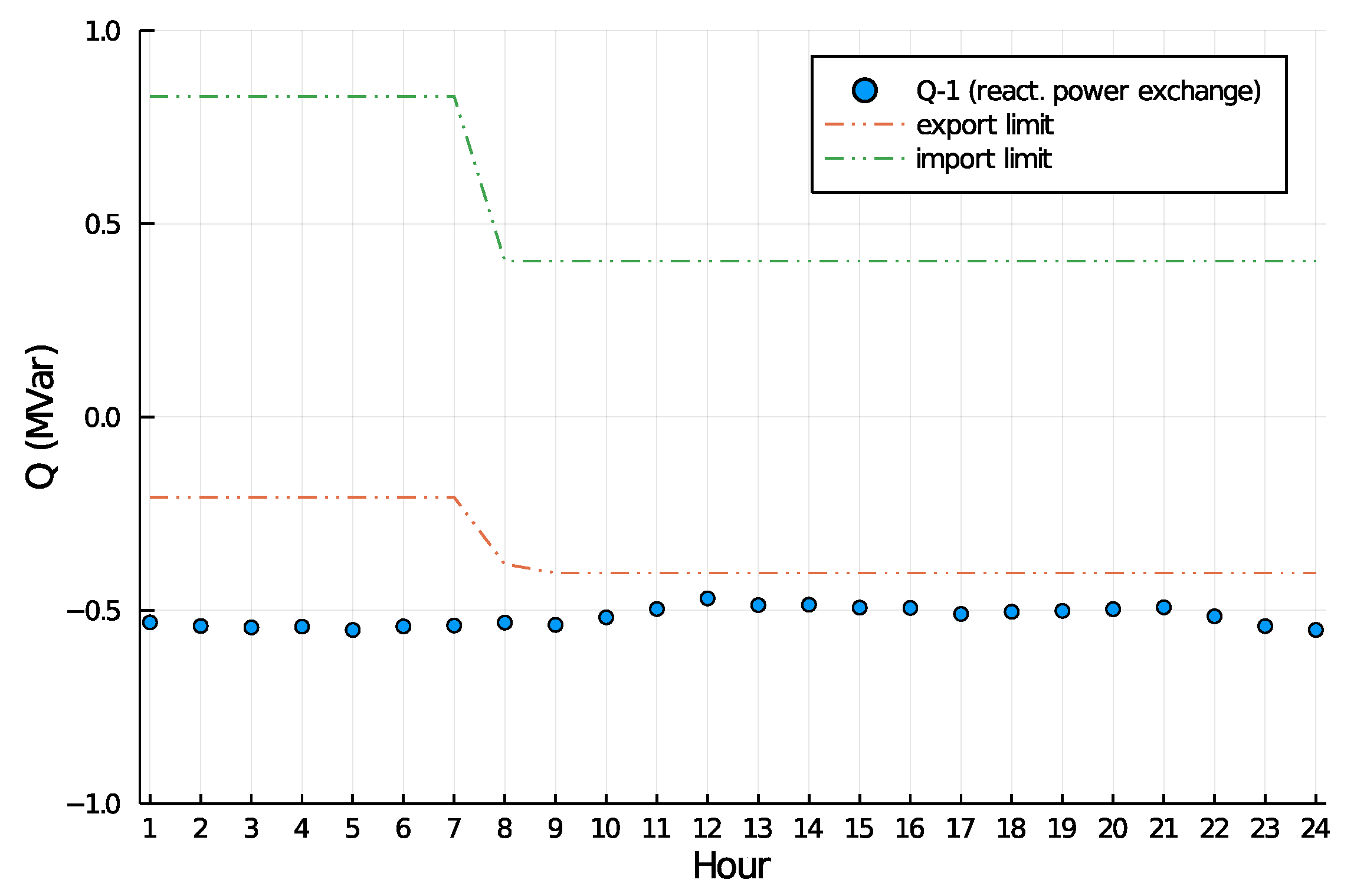
3.4. Results, Full Day

Figure 10 depicts the average active power exchange with the transmission network for each hour of the day. The first seven hours belong to the third region ( r = 3 ) of Figure 1, i.e., reactive power export limit is Q D 1 . Hour 8 belongs to the second region ( r = 2 ), while the rest of the day belongs to the first region ( r = 1 ), see also Figure 11. The pattern indicates that the distribution network is importing power from the transmission system until the 7th hour, but it is apparent that load is low. As morning progresses, power from PVs is ramping up, and for the 8th hour, the average power exchange is such that the average reactive power exchange limit is set in r = 2 , where it is a linear function of the active power. Then, PV generation is ramping up more but wind power is temporarily reduced, see hours 9–11. However, the exchange is such that r = 3 limits are applied on reactive power exchange and stay as such for the rest of the day. From hour 12, wind power ramps up again and is added to the PV generation which fluctuates along with the natural irradiation levels of a summer day leading to a day with significant export of reactive power, especially around noon.
Figure 11 illustrates how the average active power exchange of Figure 10 impacts the limits on reactive power along with the average reactive power under the zero case, i.e., no reactive power support from DERs. It is apparent that without support, the low load conditions lead to reactive power flowing from the distribution network to the transmission network, exceeding respective limits of each hour. Night hours are the worst in terms of violation, as due to the limits being in the 3rd region ( r = 3 ), the reactive power export limit is stricter that the rest of the day.
Figure 12 shows the reactive power exchange under the benchmark case of the QV droop curve. We see that violation of the exchange limit happens in considerably fewer hours than the zero case. However, one can observe that in the first seven hours no improvement occurs. This is due to low generation from both the WT and the PV, which in turns leads to minimal voltage raise and consequently no contribution by the QV droop. Additionally, the import limit is reached during hours of abundant WT and PV generation later in the day due to the significant voltage rise this large generation creates.
Figure 13 illustrates the reactive power exchange when the proposed method is used. One can observe that the limits are respected for all hours. Compared to the benchmark, the method succeeds in addressing the limit violations during night hours. This is because it does not react to temporary and local information, such as the voltage at the DER nodes, in order to provide reactive power support. Instead, the control algorithm, having an overview of the entire system and the horizon, actively instructs the DERs to provide any available support in order to solve a remote (spatially and temporally) problem, such as the violation of the average reactive power export limits at the end of the hour. Moreover, it employs the minimum volume of reactive support, marginally keeping the system within limits. In contrast, the QV droop uses significantly more reactive power support, leading in occasion to a violation of the import limits, instead (e.g., see hour 15 in Figure 12). More specifically, with the proposed method, the total reactive power support from DER is 49.56 kVARh, while under the benchmark case it is 123.33 kVARh. This is a reduction of 60%.

4. Conclusions

This paper addresses the problem of compliance of distribution systems with transmission system requirements with regards to keeping reactive power flows within limits. This objective is achieved by exploiting DER reactive power support capabilities. Compared to relevant literature, the main contribution of this work lies in the implementation of complex requirements, as the ones imposed by the Finish TSO, Fingrid. Previous approaches of the same problem have proposed a controller that in real-time reacts to the conditions on the HV/MV connection points. This paper proposes an optimisation method that considers a detailed grid model and can act predictively to the upcoming network conditions. The method relies on a quadratic program that can be efficiently solved by commercial solvers and is easily formulated into a MPC equivalent.
Results show that the proposed method achieves DN compliance with TSO limits on reactive power exchange. Compared to the benchmark case, the proposed method achieves 100% compliance to the distribution system’s reactive power import/export limits imposed by TSO requirements, compared to only 42% compliance by the benchmark QV droop method. Moreover, the proposed method utilises 60% less reactive power support from DERs. Finally, the execution time of each instance of the method is under a second, rendering it perfectly satisfactory for the requirements of the problem.

Author Contributions

Conceptualization, K.S., P.P. and N.H.; methodology, P.P. and N.H.; software, P.P.; validation, P.P. and N.H.; formal analysis, P.P.; investigation, P.P., N.H. and K.S.; resources, K.S. and P.P.; data curation, K.S. and P.P.; writing—original draft preparation, P.P.; writing—review and editing, P.P.; K.S., C.Z., N.H., K.K. and H.L.; visualization, P.P., N.H. and C.Z.; supervision, N.H.; project administration, N.H.; funding acquisition, K.S., K.K. and H.L. All authors have read and agreed to the published version of the manuscript.

Funding

Part of this work was carried out in the SolarX research project with financial support provided by Business Finland, 2019–2021 (grant No. 6844/31/2018).

Conflicts of Interest

The authors declare no conflict of interest.

References

  1. Pediaditis, P.; Ziras, C.; Hu, J.; You, S.; Hatziargyriou, N. Decentralized DLMPs with synergetic resource optimization and convergence acceleration. Electr. Power Syst. Res. 2020, 187, 106467. [Google Scholar] [CrossRef]
  2. Cuffe, P.; Smith, P.; Keane, A. Capability Chart for Distributed Reactive Power Resources. IEEE Trans. Power Syst. 2014, 29, 15–22. [Google Scholar] [CrossRef]
  3. Stanković, S.; Söder, L. Analytical Estimation of Reactive Power Capability of a Radial Distribution System. IEEE Trans. Power Syst. 2018, 33, 6131–6141. [Google Scholar] [CrossRef]
  4. Cabadag, R.I.; Schmidt, U.; Schegner, P. Reactive power capability of a sub-transmission grid using real-time embedded particle swarm optimization. In Proceedings of the IEEE PES Innovative Smart Grid Technologies, Istanbul, Turkey, 12–15 October 2014; pp. 1–6. [Google Scholar]
  5. Morin, J.; Colas, F.; Guillaud, X.; Grenard, S.; Dieulot, J.Y. Rules based voltage control for distribution networks combined with TSO- DSO reactive power exchanges limitations. In Proceedings of the 2015 IEEE Eindhoven PowerTech, Eindhoven, The Netherlands, 29 June–2 July 2015; pp. 1–6. [Google Scholar]
  6. Stock, D.S.; Venzke, A.; Hennig, T.; Hofmann, L. Model predictive control for reactive power management in transmission connected distribution grids. In Proceedings of the 2016 IEEE PES Asia-Pacific Power and Energy Engineering Conference (APPEEC), Xi’an, China, 25–28 October 2016; pp. 419–423. [Google Scholar]
  7. Stock, D.S.; Sala, F.; Berizzi, A.; Hofmann, L. Optimal Control of Wind Farms for Coordinated TSO-DSO Reactive Power Management. Energies 2018, 11, 173. [Google Scholar] [CrossRef] [Green Version]
  8. Wang, H.; Kraiczy, M.; Schmidt, S.; Wirtz, F.; Toebermann, C.; Ernst, B.; Kaempf, E.; Braun, M. Reactive Power Management at the Network Interface of EHV- and HV Level. In Proceedings of the International ETG Congress 2017, Bonn, Germany, 28–29 November 2017; pp. 1–6. [Google Scholar]
  9. Buire, J.; Colas, F.; Dieulot, J.Y.; Guillaud, X. Stochastic Optimization of PQ Powers at the Interface between Distribution and Transmission Grids. Energies 2019, 12, 4057. [Google Scholar] [CrossRef] [Green Version]
  10. Finland’s Trasmission System Operateor (FINGRID). Supply of Reactive Power and Maintenance of Reactive Power Reserves. 2021. Available online: https://www.fingrid.fi/globalassets/dokumentit/en/customers/power-transmission/supply-of-reactive-power-and-maintenance-of-reactive-power-reserves-2021-id-269130.pdf (accessed on 31 May 2021).
  11. Sirviö, K.; Laaksonen, H.; Kauhaniemi, K. Active Network Management Scheme for Reactive Power Control. In Proceedings of the CIRED Workshop 2018 on Microgirds and Local Energy Communities, Ljubljana, Slovenia, 7–8 June 2018. [Google Scholar]
  12. EU. Network Code on Demand Connection; EU: Brussels, Belgium, 2016. [Google Scholar]
  13. Finland’s Trasmission System Operateor (FINGRID). Supply of Reactive Power and Maintenance of Reactive Power Reserves; FINGRID: Helsinki, Finland, 2017. [Google Scholar]
  14. Laaksonen, H.; Hovila, P. Flexzone concept to enable resilient distribution grids—Possibilities in Sundom Smart Grid. In Proceedings of the CIRED Workshop 2016, Helsinki, Finland, 14–15 June 2016; pp. 1–4. [Google Scholar]
  15. Laaksonen, H.; Hovila, P. Future-proof islanding detection schemes in Sundom Smart Grid. CIRED Open Access Proc. J. 2017, 2017, 1777–1781. [Google Scholar] [CrossRef] [Green Version]
  16. Uebermasser, S. Requirements for coordinated ancillary services covering different voltage levels. CIRED Open Access Proc. J. 2017, 2017, 1421–1424. [Google Scholar] [CrossRef]
  17. Sirviö, K.; Mekkanen, M.; Kauhaniemi, K.; Laaksonen, H.; Salo, A.; Castro, F.; Ansari, S.; Babazadeh, D. Controller Development for Reactive Power Flow Management Between DSO and TSO Networks. In Proceedings of the 2019 IEEE PES Innovative Smart Grid Technologies Europe (ISGT-Europe), Bucharest, Romania, 29 September–2 October 2019; pp. 1–5. [Google Scholar]
  18. Sirviö, K.; Mekkanen, M.; Kauhaniemi, K.; Laaksonen, H.; Salo, A.; Castro, F.; Ansari, S.; Babazadeh, D. Testing an IEC 61850-based Light-weighted Controller for Reactive Power Management in Smart Distribution Grids. In Proceedings of the IECON 2019—45th Annual Conference of the IEEE Industrial Electronics Society, Lisbon, Portugal, 14–17 October 2019; Volume 1, pp. 6469–6474. [Google Scholar]
  19. Sirviö, K.; Mekkanen, M.; Kauhaniemi, K.; Laaksonen, H.; Salo, A.; Castro, F.; Babazadeh, D. Accelerated Real-Time Simulations for Testing a Reactive Power Flow Controller in Long-Term Case Studies. J. Electr. Comput. Eng. 2020, 2020, 8265373. [Google Scholar] [CrossRef]
  20. Baran, M.; Wu, F. Network reconfiguration in distribution systems for loss reduction and load balancing. IEEE Trans. Power Deliv. 1989, 4, 1401–1407. [Google Scholar] [CrossRef]
  21. Boyd, S.; Vandenberghe, L. Convex Optimization; Cambridge University Press: Cambridge, MA, USA, 2004. [Google Scholar]
  22. Šulc, P.; Backhaus, S.; Chertkov, M. Optimal Distributed Control of Reactive Power Via the Alternating Direction Method of Multipliers. IEEE Trans. Energy Convers. 2014, 29, 968–977. [Google Scholar] [CrossRef] [Green Version]
  23. Bezanson, J.; Edelman, A.; Karpinski, S.; Shah, V.B. Julia: A fresh approach to numerical computing. SIAM Rev. 2017, 59, 65–98. [Google Scholar] [CrossRef] [Green Version]
  24. Dunning, I.; Huchette, J.; Lubin, M. JuMP: A Modeling Language for Mathematical Optimization. SIAM Rev. 2017, 59, 295–320. [Google Scholar] [CrossRef]
  25. Gurobi Optimization, LLC. Gurobi Optimizer Reference Manual; Gurobi Optimization, LLC: Houston, TX, USA, 2021. [Google Scholar]
  26. Laaksonen, H.; Sirviö, K.; Aflecht, S.; Hovila, P. Multi-objective active network management scheme studied in Sundom smart grid with MV and LV network connected DER units. In Proceedings of the 25th International Conference on Electricity Distribution: CIRED 2019, Madrid, Spain, 3–6 June 2019. [Google Scholar]
Figure 1. TSO guidelines regarding power exchange with a DN. Input stands for exporting power from the distribution to the transmission and output stands for export [10].
Applsci 11 07719 g001
Figure 2. Illustration of part of the distribution network.
Applsci 11 07719 g002
Figure 3. Regions of the TSO guidelines regarding power exchange with a DN.
Applsci 11 07719 g003
Figure 4. Flow chart of the proposed method.
Applsci 11 07719 g004
Figure 5. Sundom network.
Applsci 11 07719 g005
Figure 6. Measured reactive power exchange between Sundom and the transmission system with respect to the limits set by the TSO. The positive sign indicates power flow from the transmission to the distribution system.
Applsci 11 07719 g006
Figure 7. Droop curve tested during studies for the Sundom pilot site, presented in [26].
Applsci 11 07719 g007
Figure 8. Evolution of the average reactive power exchange Q ^ 1 , τ , and the corresponding import/export TSO requirement limits until time step τ during the 8th hour of the chosen day using the proposed method (Q-1—proposed), the QV droop (Q-1 QV droop) and the zero case (Q-1—zero case).
Applsci 11 07719 g008
Figure 9. Reactive power support from the DERs for each time step τ during the 8th hour of the chosen day and the corresponding voltage at one of the nodes with DER.
Applsci 11 07719 g009
Figure 10. Active power exchange with the transmission system for the day under test in the case study.
Applsci 11 07719 g010
Figure 11. Reactive power exchange with the transmission system for the entire day when no reactive power support from DER is utilised (zero case).
Applsci 11 07719 g011
Figure 12. Reactive power exchange with the transmission system for the entire day when a QV droop curve support scheme is used (benchmark case).
Applsci 11 07719 g012
Figure 13. Reactive power exchange with the transmission system for the entire day when the proposed method is used.
Applsci 11 07719 g013
Table 1. Minimum and maximum values of active and reactive power of load profiles.
Node234567912
min P (MW)0.080.00.00.120.150.00.200.02
max P (MW)0.220.00.00.370.470.00.730.07
min Q (MVar)−0.060.00.0−0.09−0.090.0−0.22−0.06
max Q (MVar)−0.040.00.0−0.06−0.050.0−0.14−0.05
Table 2. Installed capacity of DERs.
DER (Node)PV (10)WT (10)
Capacity (MW)0.63.5
Publisher’s Note: MDPI stays neutral with regard to jurisdictional claims in published maps and institutional affiliations.

