
Research on Fish Slicing Method Based on Simulated Annealing Algorithm


Abstract
:1. Introduction
2. Problem Description
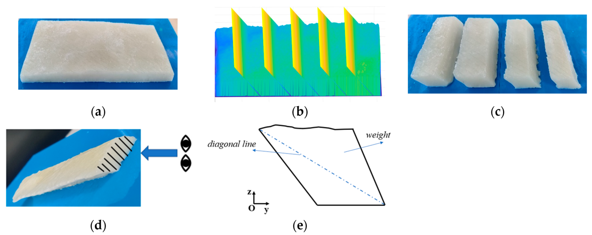
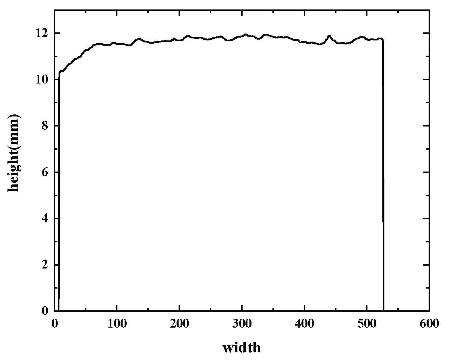
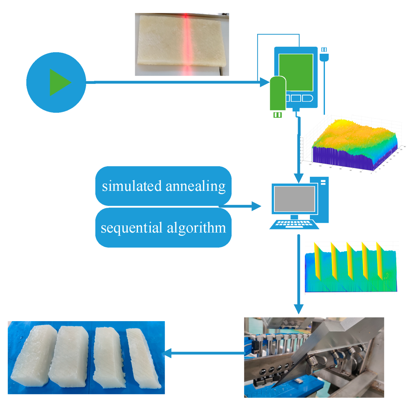
2.1. Data Acquisition
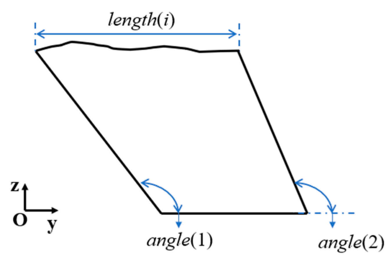
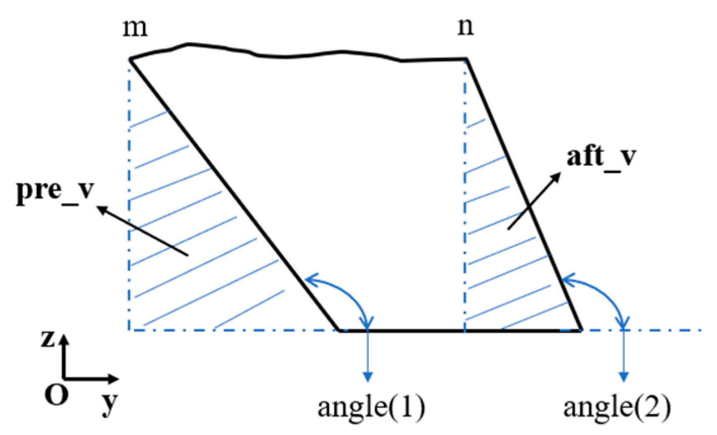
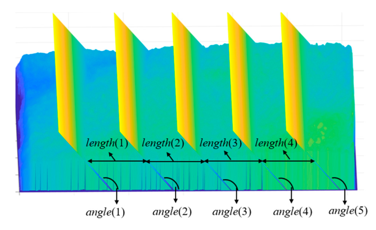
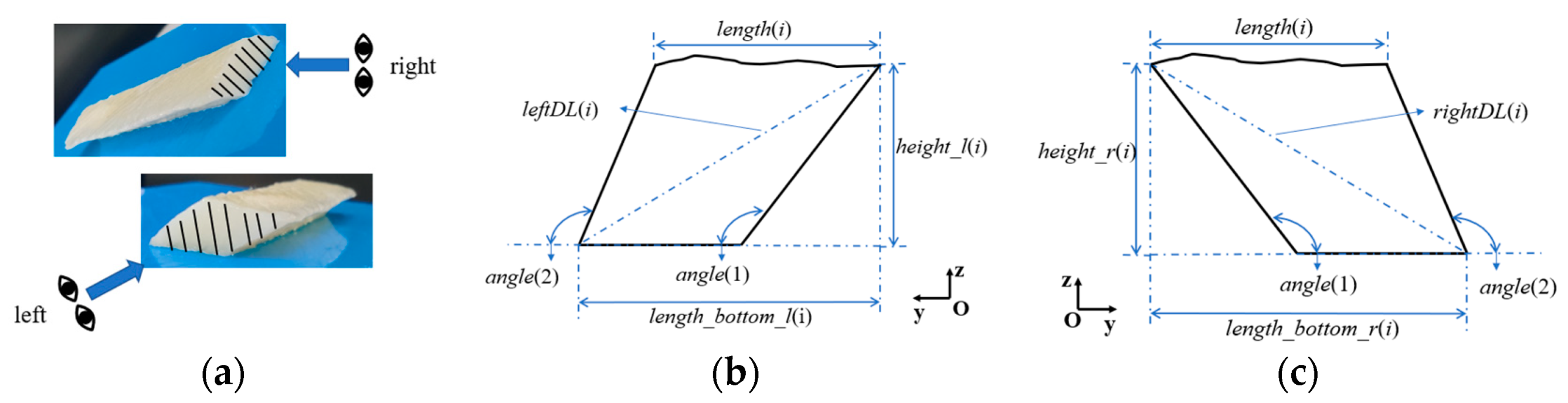
2.2. Parameter Calculation
2.2.1. Determination of errorW
2.2.2. Determination of errorDL
2.3. Object Function
3. SA algorithm for the Cutting Problem
3.1. Selection of an Intelligent Algorithm
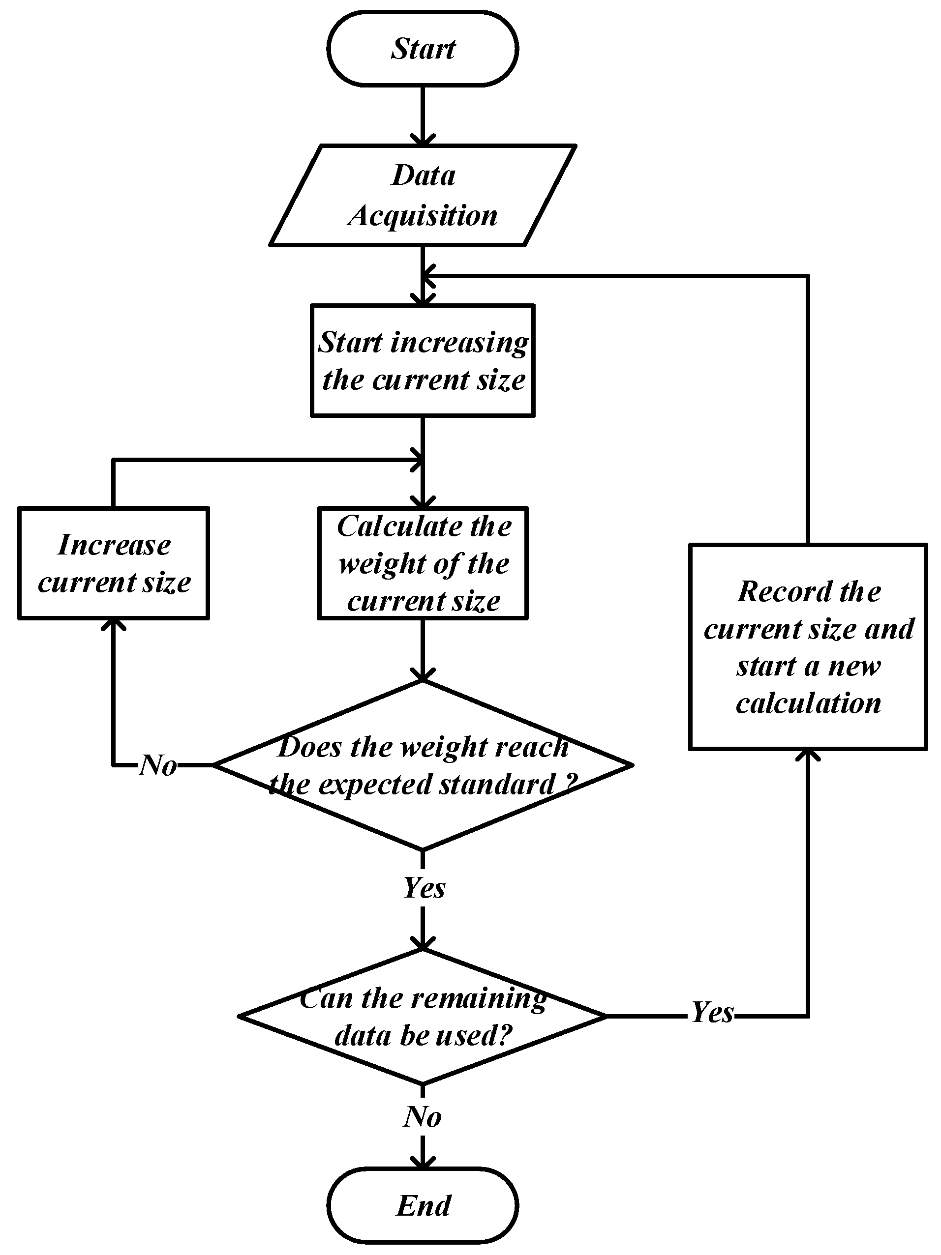
3.2. Cutting Algorithm
| Algorithm 1: SA algorithm | |
| Input: number of iterations iter; initial temperature T; current solution; inner loop | |
| Output: best solution | |
| 1. | iter=0 |
| 2. | initialise T |
| 3. | stop criterion = maximum number of iterations |
| 4. | initialise current solution |
| 5. | current cost = Evaluate(current solution) |
| 6. | while not stop criterion do |
| 7. | while inner loop do |
| 8. | Neighbour = Generate(current solution) |
| 9. | Neighbour cost = Evaluate(Neighbour) |
| 10. | if Accept(current cost, Neighbour cost, T) |
| 11. | current solution = Neighbour |
| 12. | Current cost = Neighbour cost |
| 13. | end |
| 14. | Update(best solution, iter) |
| 15. | end |
| 16. | Update(T) |
| 17. | Update(stop criterion) |
| 18. | end |
| 19. | return best solution |
- Initial solution
- Since the cuts must be continuously distributed throughout the fish body, the starting position of the initial solution must be determined, which is determined by the algorithm’s preprocessing strategy. After determining the starting position, use the real number vector to establish the initial solution, the size of which is 2n + 1, that is, X = [x1, x2, …, x2n + 1]. The first n elements are the length of each small piece, and the n + 1th to 2n+1th elements are the cutting angles of the front and back sides of each small piece, so X can also be expressed as [length(1)…length(n), angle(1)…angle(n+1)].
- Generation of new solutions
- Metropolis Guidelines
- Cool down
4. Results and Discussions
4.1. Implementation on Real Data
4.1.1. Sequential Algorithm
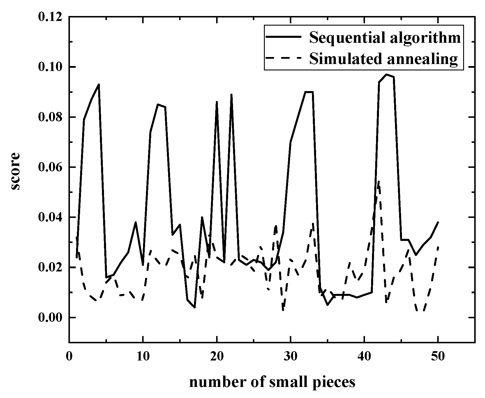
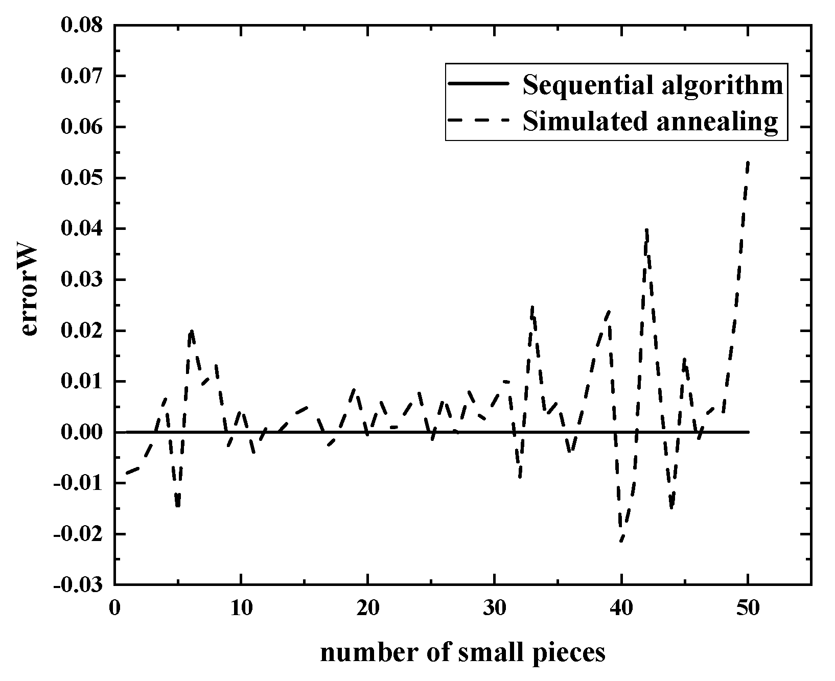
4.1.2. Results of the Two Algorithms
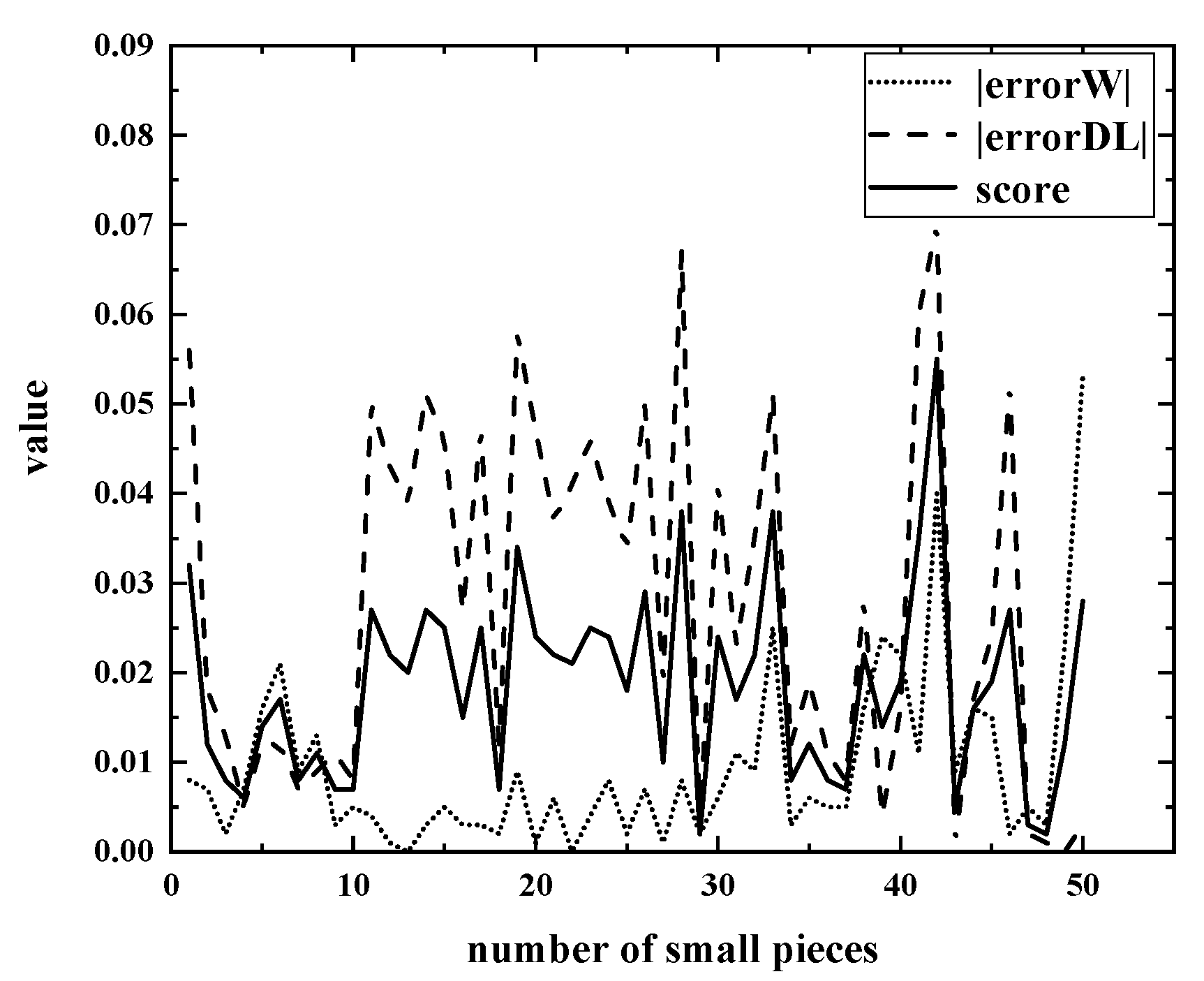
4.2. Error Analysis
5. Conclusions
Author Contributions
Funding
Institutional Review Board Statement
Informed Consent Statement
Data Availability Statement
Acknowledgments
Conflicts of Interest
References
- Decker, M.; Fischer, M.; Ott, I. Service Robotics and Human Labor: A first technology assessment of substitution and cooperation. Robot. Auton. Syst. 2017, 87, 348–354. [Google Scholar] [CrossRef] [Green Version]
- Teigland, R.; van der Zande, J.; Teigland, K.; Siri, S. The Substitution of Labor from Technological Feasibility to Other Factors Influencing Job Automation; Stockholm School of Economics Institute for Research: Stockholm, Sweden, 2018. [Google Scholar]
- Omar, F.; de Silva, C.W. Estimation of the weight distribution function of a complex object for portion control in an innovative can filling system. In Proceedings of the American Control Conference, Albuquerque, NM, USA, 4–6 June 1997; IEEE: Piscataway, NJ, USA, 1997. [Google Scholar]
- Omar, F.; de Silva, C.W. High-speed model-based weight sensing of complex objects with application in industrial processes. Measurement 2003, 33, 23–33. [Google Scholar] [CrossRef]
- Dibet Garcia Gonzalez, N.A.; Figueiredo, R.; Maia, P.; Lopez, M.A.G. Automated vision system for cutting fixed-weight or fixed-length frozen fish portions. In Proceedings of the 8th International Conference on Pattern Recognition Applications and Methods, Prague, Czech Republic, 19–21 February 2019; Springer: New York, NY, USA, 2020. [Google Scholar]
- Arkhipkin, A.I.; Rodhouse, P.G.; Pierce, G.J.; Sauer, W.; Sakai, M.; Allcock, L.; Arguelles, J.; Bower, J.R.; Castillo, G.; Ceriola, L.; et al. World squid fisheries. Rev. Fish. Sci. Aquac. 2015, 23, 92–252. [Google Scholar] [CrossRef] [Green Version]
- Melega, G.M.; de Araujo, S.A.; Jans, R. Classification and literature review of integrated lot-sizing and cutting stock problems. Eur. J. Oper. Res. 2018, 271, 1–19. [Google Scholar] [CrossRef] [Green Version]
- Russo, M.; Boccia, M.; Sforza, A.; Sterle, C. Constrained two-dimensional guillotine cutting problem: Upper-bound review and categorization. Int. T. Oper. Res. 2020, 27, 794–834. [Google Scholar] [CrossRef]
- Ozdamar, L. The cutting-wrapping problem in the textile industry: Optimal overlap of fabric lengths and defects for maximizing return based on quality. Int. J. Prod. Res. 2010, 38, 1287–1309. [Google Scholar] [CrossRef]
- Yanasse, H.H.; Limeira, M.S. A hybrid heuristic to reduce the number of different patterns in cutting stock problems. Comput. Oper. Res. 2006, 33, 2744–2756. [Google Scholar] [CrossRef]
- Golfeto, R.R.; Moretti, A.C.; Salles Neto, L.L.I.N. A genetic symbiotic algorithm applied to the one-dimensional cutting stock problem. Pesqui. Oper. 2009, 29, 365–382. [Google Scholar] [CrossRef] [Green Version]
- Cui, Y.; Liu, Z. C-Sets-based sequential heuristic procedure for the one-dimensional cutting stock problem with pattern reduction. Optim. Method. Softw. 2011, 26, 155–167. [Google Scholar] [CrossRef]
- Mobasher, A.; Ekici, A. Solution approaches for the cutting stock problem with setup cost. Comput. Oper. Res. 2013, 40, 225–235. [Google Scholar] [CrossRef]
- Araujo, S.A.D.; Poldi, K.C.; Smith, J. A genetic algorithm for the one-dimensional cutting stock problem with setups. Pesqui. Oper. 2014, 34, 165–187. [Google Scholar] [CrossRef] [Green Version]
- Rönnqvist, M. Optimization in forestry. Math. Program. 2003, 97, 267–284. [Google Scholar] [CrossRef]
- Coello, C.A.C.; Lamont, G.B.; Van Veldhuizen, D.A. Evolutionary Algorithms for Solving Multi-Objective Problems; Springer: New York, NY, USA, 2007. [Google Scholar]
- Bezerra, V.M.; Leao, A.A.; Oliveira, J.E.F.; Santos, M.O. Models for the two-dimensional level strip packing problem—A review and a computational evaluation. J. Oper. Res. Soc. 2020, 71, 606–627. [Google Scholar] [CrossRef]
- Jinqiu, Y. The Models for Estimating the Performance of Intelligence Optimization Algorithms; Zhejiang University: Hangzhou, China, 2011. [Google Scholar]
- Yongchao, G. Study on Performance of Intelligent Optimization Algorithms and Search Space; Shandong University: Jinan, China, 2007. [Google Scholar]


| Symbol | Description |
|---|---|
| w, l, h | volume element unit (length, width, height) |
| idealVol | expected volume of small piece |
| idealDL | expected diagonal length of small piece |
| n | maximum number of pieces of the whole raw material |
| length(i) | The length of the i-th piece |
| angle(i), angle(i+1) | front and back cutting angle of the i-th piece |
| realVol(i) | the actual cutting volume of the i-th piece |
| rightDL(i) | the length of the right diagonal of the i-th piece |
| leftDL(i) | the left diagonal length of the i-th piece |
| score(i) | the score of the i-th piece |
| Score | the sum of the scores of all pieces |
| Sequential Algorithm | Simulated Annealing | ||||||||||
|---|---|---|---|---|---|---|---|---|---|---|---|
| n | P1 1 | P2 2 | n | P1 | P2 | n | P1 | P2 | n | P1 | P2 |
| 1 | 0 | −0.048 | 26 | 0 | 0.044 | 1 | −0.008 | −0.056 | 26 | 0.007 | −0.05 |
| 2 | 0 | −0.157 | 27 | 0 | 0.038 | 2 | −0.007 | −0.018 | 27 | −0.001 | −0.019 |
| 3 | 0 | −0.174 | 28 | 0 | 0.045 | 3 | −0.002 | −0.013 | 28 | 0.008 | −0.067 |
| 4 | 0 | −0.185 | 29 | 0 | 0.067 | 4 | 0.007 | −0.005 | 29 | 0.002 | −0.003 |
| 5 | 0 | 0.032 | 30 | 0 | −0.141 | 5 | −0.016 | −0.012 | 30 | 0.006 | −0.041 |
| 6 | 0 | 0.034 | 31 | 0 | −0.159 | 6 | 0.021 | −0.012 | 31 | 0.011 | −0.023 |
| 7 | 0 | 0.043 | 32 | 0 | −0.181 | 7 | 0.009 | 0.007 | 32 | −0.009 | −0.035 |
| 8 | 0 | 0.052 | 33 | 0 | −0.18 | 8 | 0.013 | −0.009 | 33 | 0.025 | −0.051 |
| 9 | 0 | 0.076 | 34 | 0 | −0.023 | 9 | −0.003 | −0.011 | 34 | 0.003 | −0.012 |
| 10 | 0 | −0.042 | 35 | 0 | −0.011 | 10 | 0.005 | −0.008 | 35 | 0.006 | −0.019 |
| 11 | 0 | −0.148 | 36 | 0 | −0.018 | 11 | −0.004 | −0.05 | 36 | −0.005 | −0.011 |
| 12 | 0 | −0.17 | 37 | 0 | −0.019 | 12 | 0.001 | −0.043 | 37 | 0.005 | −0.008 |
| 13 | 0 | −0.168 | 38 | 0 | −0.018 | 13 | 0 | −0.039 | 38 | 0.016 | 0.028 |
| 14 | 0 | −0.065 | 39 | 0 | −0.017 | 14 | 0.003 | −0.051 | 39 | 0.024 | 0.004 |
| 15 | 0 | −0.074 | 40 | 0 | 0.019 | 15 | 0.005 | −0.046 | 40 | −0.022 | −0.016 |
| 16 | 0 | −0.013 | 41 | 0 | −0.02 | 16 | 0.003 | −0.027 | 41 | −0.011 | −0.06 |
| 17 | 0 | −0.009 | 42 | 0 | −0.187 | 17 | −0.003 | −0.047 | 42 | 0.04 | −0.07 |
| 18 | 0 | −0.08 | 43 | 0 | −0.193 | 18 | 0.002 | −0.012 | 43 | 0.009 | −0.001 |
| 19 | 0 | −0.048 | 44 | 0 | −0.192 | 19 | 0.009 | −0.058 | 44 | −0.016 | −0.017 |
| 20 | 0 | −0.172 | 45 | 0 | 0.062 | 20 | −0.001 | −0.047 | 45 | 0.015 | −0.024 |
| 21 | 0 | −0.044 | 46 | 0 | 0.062 | 21 | 0.006 | −0.037 | 46 | −0.002 | −0.052 |
| 22 | 0 | −0.178 | 47 | 0 | 0.049 | 22 | 0 | −0.041 | 47 | 0.005 | 0.002 |
| 23 | 0 | 0.046 | 48 | 0 | 0.058 | 23 | 0.004 | −0.046 | 48 | 0.003 | −0.001 |
| 24 | 0 | 0.043 | 49 | 0 | 0.064 | 24 | 0.008 | −0.039 | 49 | 0.023 | 0 |
| 25 | 0 | 0.046 | 50 | 0 | 0.075 | 25 | −0.002 | −0.034 | 50 | 0.053 | −0.003 |
| Parameters | Statistics | Sequential Algorithm | Simulated Annealing |
|---|---|---|---|
| errorW | maxW | 0% | 5.31% |
| minW | 0% | −2.16% | |
| avgW | 0% | 0.49% | |
| stdW | 0% | 1.3% | |
| rateW | 100% | 98% | |
| errorDL | maxDL | 7.59% | 2.83% |
| minDL | −19.32% | −6.96% | |
| avgDL | −4.36% | −2.61% | |
| stdDL | 9.4% | 2.25% | |
| rateDL | 48% | 90% |
| maxSc | minSc | avgSc | stdSc | rateSc | |
|---|---|---|---|---|---|
| Sequential algorithm | 9.66% | 0.44% | 4.09% | 3.14% | 70% |
| Simulated annealing | 5.49% | 0.22% | 1.86% | 1.09% | 96% |
| A | B | C | D | |
|---|---|---|---|---|
| percent | 50% | 46% | 2% | 2% |
Publisher’s Note: MDPI stays neutral with regard to jurisdictional claims in published maps and institutional affiliations. |
© 2021 by the authors. Licensee MDPI, Basel, Switzerland. This article is an open access article distributed under the terms and conditions of the Creative Commons Attribution (CC BY) license (https://creativecommons.org/licenses/by/4.0/).
Share and Cite
Liu, S.; Wang, H.; Cai, Y. Research on Fish Slicing Method Based on Simulated Annealing Algorithm. Appl. Sci. 2021, 11, 6503. https://doi.org/10.3390/app11146503
Liu S, Wang H, Cai Y. Research on Fish Slicing Method Based on Simulated Annealing Algorithm. Applied Sciences. 2021; 11(14):6503. https://doi.org/10.3390/app11146503
Chicago/Turabian StyleLiu, Shuo, Hao Wang, and Yong Cai. 2021. "Research on Fish Slicing Method Based on Simulated Annealing Algorithm" Applied Sciences 11, no. 14: 6503. https://doi.org/10.3390/app11146503
APA StyleLiu, S., Wang, H., & Cai, Y. (2021). Research on Fish Slicing Method Based on Simulated Annealing Algorithm. Applied Sciences, 11(14), 6503. https://doi.org/10.3390/app11146503