Abstract
Despite being heavily used in the training of deep neural networks (DNNs), multipliers are resource-intensive and insufficient in many different scenarios. Previous discoveries have revealed the superiority when activation functions, such as the sigmoid, are calculated by shift-and-add operations, although they fail to remove multiplications in training altogether. In this paper, we propose an innovative approach that can convert all multiplications in the forward and backward inferences of DNNs into shift-and-add operations. Because the model parameters and backpropagated errors of a large DNN model are typically clustered around zero, these values can be approximated by their sine values. Multiplications between the weights and error signals are transferred to multiplications of their sine values, which are replaceable with simpler operations with the help of the product to sum formula. In addition, a rectified sine activation function is utilized for further converting layer inputs into sine values. In this way, the original multiplication-intensive operations can be computed through simple add-and-shift operations. This trigonometric approximation method provides an efficient training and inference alternative for devices with insufficient hardware multipliers. Experimental results demonstrate that this method is able to obtain a performance close to that of classical training algorithms. The approach we propose sheds new light on future hardware customization research for machine learning.
1. Introduction
Deep neural networks (DNNs), of strong fitting capabilities, have extended the range of application of artificial intelligence in recent years. In the face of increasingly complicated learning tasks, researchers have deepened and widened neural networks to achieve better representation capabilities. The price of this increased capability is a large consumption of computing resources, which poses a hefty challenge to hardware design.
As neural networks increase in size, the training of the neural network becomes more dependent on specialized hardware consisting of thousands of computing units. General matrix multiply (GEMM) is at the core of deep learning because a tremendous amount of matrix multiplication operations are required for neural network training. To accelerate the training and inference of deep neural networks, hardware vendors are constantly increasing the chip area and the number of processing units. Nevertheless, accelerating matrix multiplication operations remains cost-ineffective, in contrast to accelerating simple operations, such as addition, subtraction, and a bit shift.
In terms of hardware implementation, multipliers are bulky and power-intensive compared to other logic resources. Consequently, this prohibits deployment to scenarios when the multipliers are insufficient. For instance, digital signal processing (DSP) used for floating-point multiplication is often found to be a scarce resource when attempting to implement neural networks on field-programmable gate arrays (FPGAs). To reduce the usage of hardware multipliers, many researchers use a coordinate rotation digital computer (CORDIC) [1]) module to compute layer activations rather than the direct usage of DSPs on FPGAs when hyperbolic activation functions are applied. This method involves only additions, subtractions, a bit shift, and look-up tables, and has been confirmed to be more hardware efficient [2,3,4]. Although widely used in microcontrollers and FPGAs, CORDIC can only partially eliminate dependence on multipliers, and a large number of multipliers are still required for inference and error backpropagation, which hinders on-FPGA neural network training.
Efforts had been put into hardware optimizations. Many optimization possibilities are motivated by the various inherent characteristics of the CNN models. For instance, CNN’s spatially correlated characteristics, i.e., adjacent output feature map activations will share close values per feature map, motivated Shomron et al. to propose a value prediction based method that reduces MAC operations [5] in DNNs. In [6], a lightweight CNN is implemented to predict zero-valued activations. The prediction step is calculated prior to the convolution step, thus the convolution operations can be largely saved. In addition, the sparsity of DNN values causes the underutilization of the underlying hardware. For example, DNN tensors usually follow a bell-shaped distribution that is concentrated on zero, therefore a high percentage of values will only be represented by a portion of least-significant bits (LSBs). These zero-valued bits may cause inefficiencies when executed on hardware. To address it, a non-blocking simultaneous multithreading (NB-SMT) method [7] was designed to better utilize the execution resources. Many quantization algorithms have also been proposed to reduce the usage of multipliers in DNNs. For example, to quantize all network weights into powers of 2, one can avoid multiplications [8]. However, the calculation of weight parameters directly involved only accounts for a part of the neural network training. If we further quantize the layer inputs, we can reduce the use of multipliers to a greater extent, which will cause a huge accuracy loss and is only suitable for simple tasks [9]. For circumstances in which hardware multipliers are insufficient, we propose a trigonometric approach to eliminate the dependence on multipliers.
Consider a simple case in which only fully connected layers are used, and the non-linearity is omitted. As shown in Figure 1, to back propagate error signals, each layer conducts multiplications between the weight matrix and error matrix from the last layer (see subfigure (b)). In addition, to update the weights, the dot product of the activation and error matrix is computed (see subfigure (c)). It is clear that multiplications between errors, activations, and weights dominate the computation cost. However, in modern neural network models, both the weight parameters and error signals are highly concentrated around zero with an extremely small variance. This characteristic enables us to approximate the original error and weight using its sine value. Then, using the product to sum formula, we can convert the multiplications to easier operations. Here, we briefly introduce the ideas behind this study.
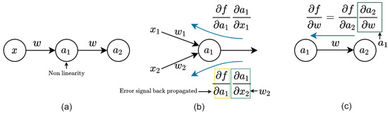
Figure 1.
A simple illustration of forward and backward inference in a neural network training. Subfigure (a) denotes the forward inference of neural networks, where non-linearity is introduced during the activation stage. Subfigure (b,c) represent the error backpropagation of neural networks. As indicated by the equations in (b,c), the error signals are backpropagated by computing the gradients of each weight by chain rule.
From Equation (1), we know that when x is infinitesimal, we regard and x as equivalent. Moreover, we have when x is a small value, and, thus, we can approximate x as . For example, the error gap is within when is smaller than 0.01. The left subfigure of Figure 2 shows a typical distribution of weight parameters extracted from a random layer of a 28-layer WideResNet trained on the CIFAR-100 dataset. The right subfigure of Figure 2 shows the error curve when we replace x with . Apparently, using the sine value as an approximation does not add much noise to the network when the parameters are highly concentrated at near 0.
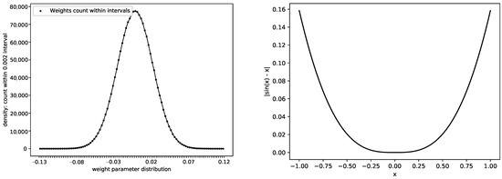
Figure 2.
Weight distribution and approximation error curve. The left subfigure shows the distribution of weight parameters extracted from a random layer of a 28-layer WideResNet trained on the CIFAR-100 dataset. The right subfigure is drawn from , which denotes the approximation error.
By applying Equation (2), i.e., the product to sum formula, we can convert multiplications of sine values into simpler addition, subtraction, and bit shift operations, which are far more economical than classical multiplication operations. Note that the cosine value can be computed by the aforementioned CORDIC engine, which is also hardware friendly and only requires simple operations. We also introduce a sine-based activation function. Rather than a mere sine activation, we adopt a rectified variant that combines the ReLU [10] and sine activation. In this way, we realize the sine value replacement of activation, error, and weight, between which the multiplications are removable in inference and training. We call this method trigonometric inference.
Trigonometric inference offers an alternative training method when the hardware multipliers are insufficient. In addition, the method is superior when a hyperbolic function, such as , is adopted as the activation function. The approach is evaluated on image classification tasks, and the experimental results confirm a performance comparable to that of the classical training method.
The remainder of this paper is organized as follows. We introduce related research in Section 2. A detailed explanation of the methodology is provided in Section 3, and Section 4 summarizes the experimental results. We discuss future work in Section 5, and some concluding remarks are provided in Section 6. Our contributions are listed as follows:
- We propose a novel training and inference method that utilizes trigonometric approximations. To the best of our knowledge, this is the first work that shows trigonometric inference can provide learning in deep neural networks;
- By replacing the model parameters and activations with their sine value, we analyze that multiplications could be transferred to shift-and-add operations in training and inference. To achieve this, a rectified sine activation function is proposed;
- We evaluate trigonometric inference on several models and shows that it can achieve performance that is close to conventional CNNs on MNIST, Cifar10, and Cifar100 datasets.
2. Related Work
Various methods have been proposed to reduce the dependence on multipliers in DNN training. We first introduce studies that approximate multiplications in DNNs with lower bit width parameters, and then discuss some studies that have replaced some of the multiplications into simpler operations, such as addition. We also investigate hardware optimizations that can reduce the use of multipliers without sacrificing parameter precision. The merits and restrictions of these methods are also detailed in this section.
2.1. Training with Low Precision
Conventional deep neural networks are trained using 32-bit parameters. The training cost can be reduced by reducing the precision of the parameters. Extreme examples in this direction are binarized neural networks (BNNs) [11] and XNOR-Net [12]. By limiting the weights and activations to 1 and −1, not only is memory consumption reduced, a large number of multiplication operations are also avoided. A BNN is suitable for devices with a weak performance, such as mobile and embedded terminals, whereas such a sacrifice results in a loss of accuracy. Moreover, the convergence of the BNN models is prolonged. A large number of training iterations cause the burden of additional training.
Models with comparatively higher precision have also been studied. It was verified that training with a lower precision does not significantly influence the accuracy of image classification. For example, Banner [13] showed that 8-bit neural networks can achieve a comparable accuracy to their full precision counterparts. In addition to image classification, efficient low-precision networks are also applicable to other tasks, such as language translation [14]. Recently, sparsity of the activations in DNNs is also utilized for quantization algorithm design. In [15], the zero value bits are leveraged to trim an 8 bits quantized value to lower n-bits resolution by picking the most significant n bits while skipping leading zero value bits.
2.2. Training with Add or Shift Operations
To avoid multiplication altogether in forward inference, Chen et al. presented an adder-based learning model [16]. Classical convolutions compute the cross-correlations between the inputs and filters. In AdderNet, the cross-correlation is replaced with the -norm distance. The experimental results confirm that this method can also extract useful features for image classification. Nevertheless, backpropagation in AdderNet still requires complicated computations consisting of multiplication, division, and square root operations to generate layer-wise learning rates.
Instead of full precision multiplications, bit-shift-based inference leads to another direction for efficient training. In 2016, Miyashita et al. proposed a logarithmic quantization algorithm [17] on neural network weights and activations to eliminate bulky digital multipliers. By converting the original weights and activations to their logarithmic data representation with a lower bit width, the memory consumption is decreased by saving only exponentials. Furthermore, multiplication is avoided because only shift operations are required. The logarithmic inference applies 3- or 4-bit quantization to pre-trained models and delivers better accuracy than linear quantization after retraining.
Elhoushi et al. proposed DeepShifs [18], which quantizes the weight to its logarithmic form in both forward and backward inference. This partly removes multiplication operations during the training stage. However, the performance increase is extremely limited because multiplication is still required in every layer during error backpropagation.
2.3. Hardware Optimization for Hyperbolic Functions with CORDIC
Hardware optimization for hyperbolic activation functions has been reported in previous studies. Although the chip area and power consumption are reduced, related studies apply hyperbolic functions only to activation computations, which limits the optimization gains. The CORDIC algorithm [1] is considered an efficient method for computing hyperbolic activations. Here, we briefly introduce the CORDIC algorithm, which is widely used in microcontrollers and FPGAs. Initially proposed in 1959, the CORDIC algorithm is an efficient way to calculate hyperbolic and trigonometric functions. A CORDIC module computes the trigonometric value of a certain angle through accumulative rotations of the preset base angles. It decomposes a certain angle into discrete base angles that are pre-stored in a look-up table. Note that all the base angles are chosen as powers of 2; thus, iterative rotations of an angle are computed through shift operations. The CORDIC algorithm then iteratively applies accumulative rotations of the base angles until the required precision is met.
Many accelerated CORDIC algorithms have been proposed over the years. For example, Jaime et al. proposed a scale-free CORDIC engine that can reduce the chip area and power consumption by 36% [19]. Mokhtar et al. proposed a sine and cosine CORDIC compute engine that requires only seven iterations for 16-bit precision [20]. An improved rotation strategy was also studied in [21], which achieved 32 precision with only approximately five iterations on average.
Chen et al. used a CORDIC engine to compute an application-specific algorithm [3], i.e., an independent component analysis (ICA), which is used for the direct separation of a number of mixed signals. In their research, only a part of the updating scalar tanh(x) was computed using the CORDIC engine. The method still relies on a comparatively large number of multipliers. A similar approach was adopted by Tiwari et al., who used CORDIC to compute activations in neural networks [22].
Another direction to take advantage of hyperbolic functions is by applying it to specific computation tasks. Heidarpur et al. utilize the CORDIC engine to compute modified Izhikevich neurons [23]. Similarly, Hao et al. realized an efficient implementation of a cerebellar Purkinje model [24].
To the best of our knowledge, there is still a lack of training algorithms that can remove the usage of multipliers on deep neural networks during the training stage.
3. Methodology
In this section, we elaborate on our trigonometric inference learning algorithm. For ease of description, we explain the algorithm based on fully connected neural networks. In convolutional models, the background idea is the same, and the only change is to replace multiplication marks with convolution marks.
3.1. Forward and Backward Inference
3.1.1. Forward Inference
Let w denotes the model weights and a activations of an arbitrary layer. Note that we use subscript j to indicate a middle layer, and i denotes the previous layer of j. Equation (3) provides the standard forward inference and Equation (4) indicates the activation calculation of our proposed trigonometric inference.
where is an activation function and is our newly proposed sine-based activation function for trigonometric inferences. A sine function has been studied as an activation function in previous studies. In 1999, Sopena et al. [25] found that a multiplayer perceptron with sine as the activation learns faster than one with sigmoid activation on certain tasks. As a significant difference, the sine is periodic, whereas common activation functions are monotonic. Parascandolo et al. [26] found that sine activation functions perform reasonably well on current datasets, and the network ignores the periodic nature of sine functions. After training, only the central region at near zero of the sine activation function was used. Ramachandran et al. [27] used automatic search techniques to discover new activation functions. They then found that activation can achieve a performance comparable to that of ReLU for image classification. Zhang et al. [28] proposed a sine-activated algorithm for a multi-input function approximation that can efficiently obtain a relatively optimal structure.
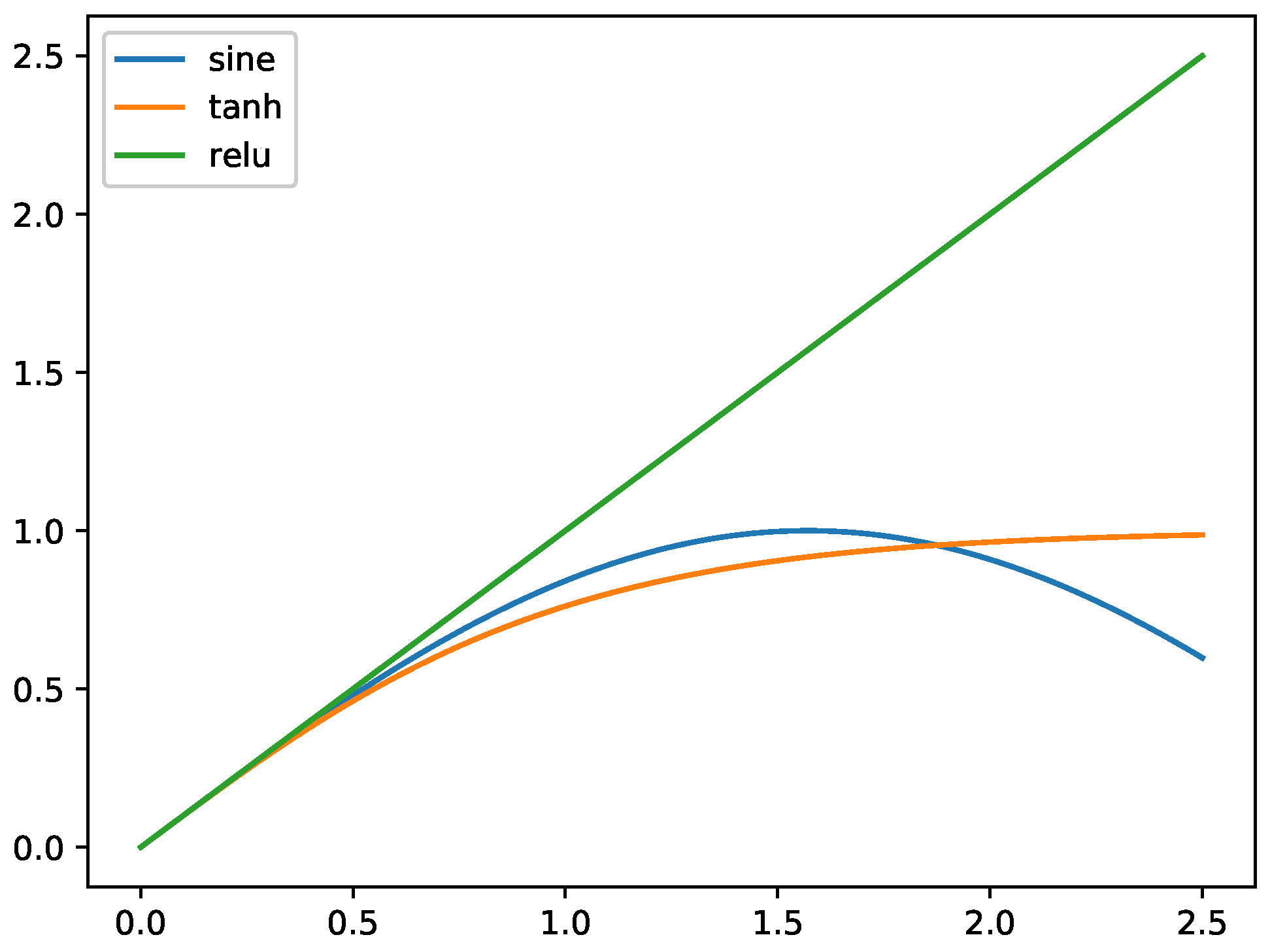
Based on previous findings, herein we propose our sine-based activation. Rather than directly applying the activation function as , we combine the ReLU activation and sine activation because this combination has two merits: First, ReLU excludes negative outputs and, therefore, the computational burden is considerably reduced. In addition, regulating the activations to only positive values can lessen the poor influence caused by the periodicity property of the sine activation. In Section 5, we show that this rectified sine activation performs much better than a pure sine activation for trigonometric training. Equation (5) gives our activation function, and from Figure 3, we know that and are extremely similar for small values.
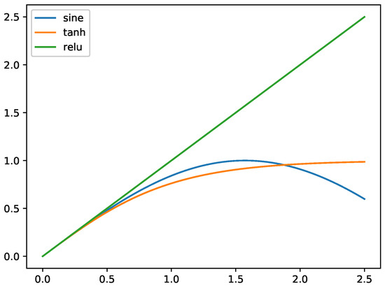
Figure 3.
Activation functions. The sine activation behaves similarly to the hyperbolic tangent activation for .
3.1.2. Backward Inference
When training a neural network, the error E calculated from the loss function is backpropagated to each layer (error backpropagation) for weight update. The weights in each layer are then updated for narrowing the error E. This parameter optimization problem can be solved using gradient descent, which requires calculating for all w in the model. Here we denoted as the backpropagated error signal from the latter layer to the layer j. According to the chain rule, we can use Equation (6) to calculate the error signal at layer i, which is backpropagated from layer j. For conventional CNNs, the error is calculated by , which equals the multiplication of and ().
For our trigonometric inference, is calculated differently since we use and to approximate x and W, respectively, in the forward pass (as Equation (4)). By taking the partial derivative of over , we get . Therefore, the error in trigonometric inference should be calculated as Equation (7) when the activation is larger than zero (Equation (5)).
Equation (7) gives the precise error signal for weight update in the middle layer i during gradient descent. However, the direct calculation of Equation (7) will incur multiplication overheads, so here we developed two methods for computing . As shown in Table 1, the mean and variance of the weights and errors are very small in a downsized VGG of eight convolutional layers. This property, which makes the approximation possible, is common in modern deep neural networks. Experimental results show the trade-off between these two approaches; here, we outline the computation details:

Table 1.
Mean and variance of convolutional layer inputs (x), weights (W), and back propagated errors (E) from the first training iteration in a downsized VGG network. Note all these mean and variance values are calculated from all x, W, E in each layer. The CIFAR-10 dataset was used, and the network contained eight convolutional layers. All mean and variance values for the weights and errors are extremely small, which enables the sine approximation of the original values.
(1) Equation (7) is divided into two parts and approximately computed. Equation (8) indicates a recursive approximation computation ( is approximated by ). In this way, multipliers are not required, and precise error signals are calculated despite the computation complexity being increased.
(2) First, we replace with in Equation (7). The above approximation strategy enables us to compute gradients using Equation (9).
Second, we use a pseudo-error signal for backpropagation. Because the cosine term in Equation (9) adds extra computational complexity, we replace it with shift operations. Since the values of the weights are generally highly concentrated around the value of zero, in an ideal situation we can simply omit the cosine term ( if ). However, in practice, we found that omitting the cosine term directly sometimes causes an excessive error, which is contributed by those weights of larger magnitude, so we replace the cosine term with 1/2. By simply scaling the original error signals to half, the algorithm provided learning in our experiments. The half-scaling strategy is formulated as in Equation (10): A similar concept was found in feedback alignment methods [29,30] for error backpropagation. Lillicrap et al. [29] discovered that the weights do not have to be symmetric in the forward and backward inferences during the training. In his research, Arild Nøkland [31] provided a theoretical analysis that supports the learning capabilities of backpropagation with pseudo-error signals.
3.1.3. Weight Update
For conventional CNNs, the learning rate ( in Equation (11)) can be set to an arbitrary value within a certain range. This may introduce an additional multiplicative burden when performing gradient descent calculations.
To avoid divisions, shift operations may be used instead when the learning rate is set to powers of 2. In this way, the divisions are converted into bit shifts.
3.2. Precision Analysis
Our training algorithm performs several approximations to significantly decrease the usage of multipliers. It omits the cosine term when the value is very small and recursively approximates small values by their sine values (Equation (10)). Here, we analyze the precision loss of the approximation strategy.
By applying the binomial theorem, we rewrite product as Equation (13) for comparison. By the Taylor theorem, is expanded to its polynomial form (Equation (14)).
where Rn(x) denotes the Lagrange form of the remainder:
The difference of Equations (13) and (14) gives the error gap of our -to- approximation. Because the term is still trigonometric, the Lagrange remainders in Equation (14) are then bounded by:
We substitute Equation (16) into and through simple unequal relations, we have the error of our approximation upper bounded by:
3.3. A Toy Example
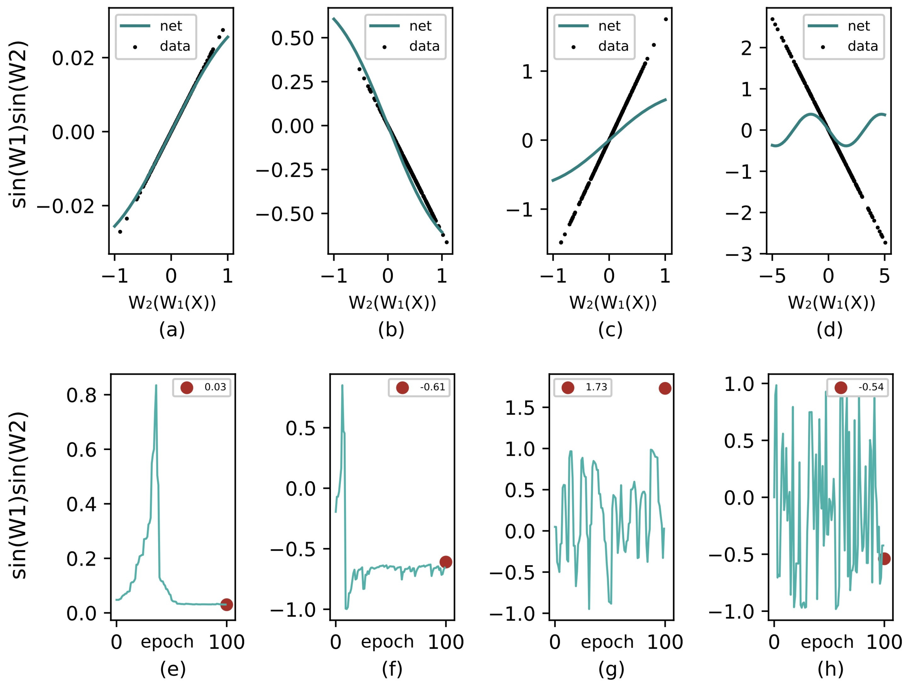
To better illustrate how the learning algorithm works, we let a simple model fit a straight line. Consider a model of only two neurons, each forming a layer, and we have a model that outputs in which the non-linearity is omitted. Using the trigonometric training method, we trained this model with different choices of parameter initials, input ranges, and target line slopes. If the target line is denoted as , the goal is to train the model that will be stable at . Figure 4 summarizes the fitting results and learning dynamics of the proposed algorithm under various conditions. The parameters for the different conditions are summarized in Table 2. In this case, the learning rate is chosen as for avoiding multipliers in the gradient descent stage (note is not required, other approximate values can work as well), and the learning dynamics subplots are drawn from the first 100 iterations. In addition, the training sample size is 300, and the final fitting curves are the results of 100 epochs of training.
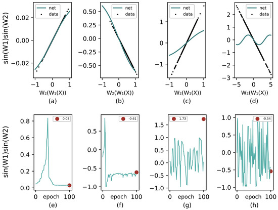
Figure 4.
Line fitting and learning dynamics of trigonometric inference under various conditions. The initial parameters for (a–d) are listed in Table 2. (a,e) represent an ideal condition in which samples are concentrated around 0. (b,f) represents a situation in which samples are drawn from comparatively large means. (c,g) depict the learning dynamics when the slope is larger than 1, which is impossible for sine activation to reach. (d,h) designate a large sample variance.
Table 2.
Initial parameters of the toy example. Note that m stands for the target slope, and denotes the mean and variance of the samples. All samples were normally distributed.
It is clear that the gradient descent functions when Equation (17) is satisfied. When the target slope is larger than 1 (see subfigure (c,g)) or sample data are drawn with large variance (subfigure (d,h)), the proposed algorithm struggles to reach the target; however, samples around 0 are still well approximated (subfigure (d)). Fortunately, in modern deep neural networks, these situations are not common and can be avoided. In addition, even if was set to 500 at the beginning, the algorithm still provided learning. Because trigonometric functions are periodic, a weight that is too large will not affect the convergence of the network.
3.4. Suitable Scenarios
Trigonometric inference allows forward and backward computations without using multipliers. It involves only simple shift-and-add operations to compute trigonometric functions when the CORDIC [1] algorithm is employed. Trigonometric inference is preferred when hardware multipliers are insufficient. Although ReLU is widely used owing to its simplicity and computational ease, many neural network models rely on hyperbolic activation functions. In FPGAs, where hardware multipliers are extremely limited resources, the CORDIC module is a more efficient alternative for computing hyperbolic activation functions [23,32]. When CORDIC modules are utilized for computing activations, a trigonometric inference is preferred because it does not require extra multipliers. By contrast, a classical training approach still requires a large number of multiplications for inference and training, even if CORDIC modules are used for activation calculations.
4. Evaluation
In this section, we use the CIFAR and MNIST datasets to test the effectiveness of the proposed learning algorithm. All computations were conducted on the CUDA devices. Note that in CUDA devices, our algorithm will have no speed gains because CUDA devices (see cuDNN [33]) and modern machine learning frameworks are specially optimized for matrix multiplication operations. We used Chainer [34] to construct the learning system and neural network models. All experiments were conducted on NVIDIA Tesla P100 and GTX1660 Super GPUs.
4.1. Experiments on MNIST
MNIST is a dataset used for handwritten digit classification. On MNIST, even a small neural network can achieve a good accuracy. By using a small neural network, we can easily adjust the model shapes to investigate the performance of a trigonometric inference under various situations. The MNIST images were 32 × 32 in size, and only fully connected layers were used to build the neural net model. In this case, we discuss the training conditions suitable for the algorithm and test the performance for different sine activations. We used a three-layer neural network and tested the convergence of the network by changing the number of intermediate neurons. The results are presented in Table 3. We use Momentum SGD to optimize the models with momentum set to 0.9 and a learning rate of 0.01. The batch size was set to 128, and no data augmentation was used. For the standard model, ReLU was used as the activation function, and as the final accuracy of the pure sine activation and the proposed rectified sine activation.
Table 3.
MNIST test accuracy.
As the results summarized in Table 3 indicate, it is noticeable that trigonometric inference fails to provide learning when the last layer size is inadequate. As the reason for this phenomenon, when the last layer size is too small, the error assigned to each connection will be too large, thus reducing the precision of the sine approximation. For comparison, confirms that trigonometric inference functions when the last layer size is sufficient. It also shows a performance decrease when small layers are adopted in the model. We also tested a model with each layer having 10,000 neurons to check the difference in performance between the proposed algorithm and the classical inference. For small neural net models with large layer sizes, the two algorithms show almost no difference, and interestingly, trigonometric inference outperforms the baseline inference method.
Rows and in Table 3 represent the validation results from a network with a full sine activation and a rectified sine activation, respectively. By comparing their final accuracy, it is clear that the proposed rectified sine activation outperforms the full sine activation by a wide margin.
4.2. Experiments on CIFAR
We then tested our method on the CIFAR-10 and CIFAR-100 datasets, each containing 60,000 RGB images. We trained a downsized VGG model [35] and a 22-layer WideResNet [36] on the CIFAR-10 and CIFAR-100 datasets. Note that Equation (8) is used for backpropagation for TrigInf 1 (method 1), and for TigInf 2 (method 2), Equation (10) is adopted. The configurations of the downsized VGG and WideResNet are shown in Table 4. For VGG, the model width was much smaller than that of the original VGG-11. By decreasing the layer width, we can observe the learning results of trigonometric inference when the network size is relatively small. We trained the model using momentum SGD with the momentum set to and decayed to half for every 25 epochs. The same training method is also used on WideResNet, in which the momentum decays every 40 epochs. The MNIST test indicates that a layer that is too narrow has a negative influence on the overall performance. Therefore, on WideResNet, we avoid using a trigonometric inference on the first layer because the number of filters is too small, which will cause a performance deterioration. We conducted trigonometric inference only on convolutional layers because they contribute the most computational burden. The batch norm was also utilized to accelerate the convergence, and all tasks were trained for 300 epochs with data augmentation. The batch size was set to 128. For comparison, we trained VGG and WideResNet without approximations. ReLU was used as the activation function for comparison groups.
Table 4.
Network configuration of the downsized VGG and the 22-layer WideResNet.
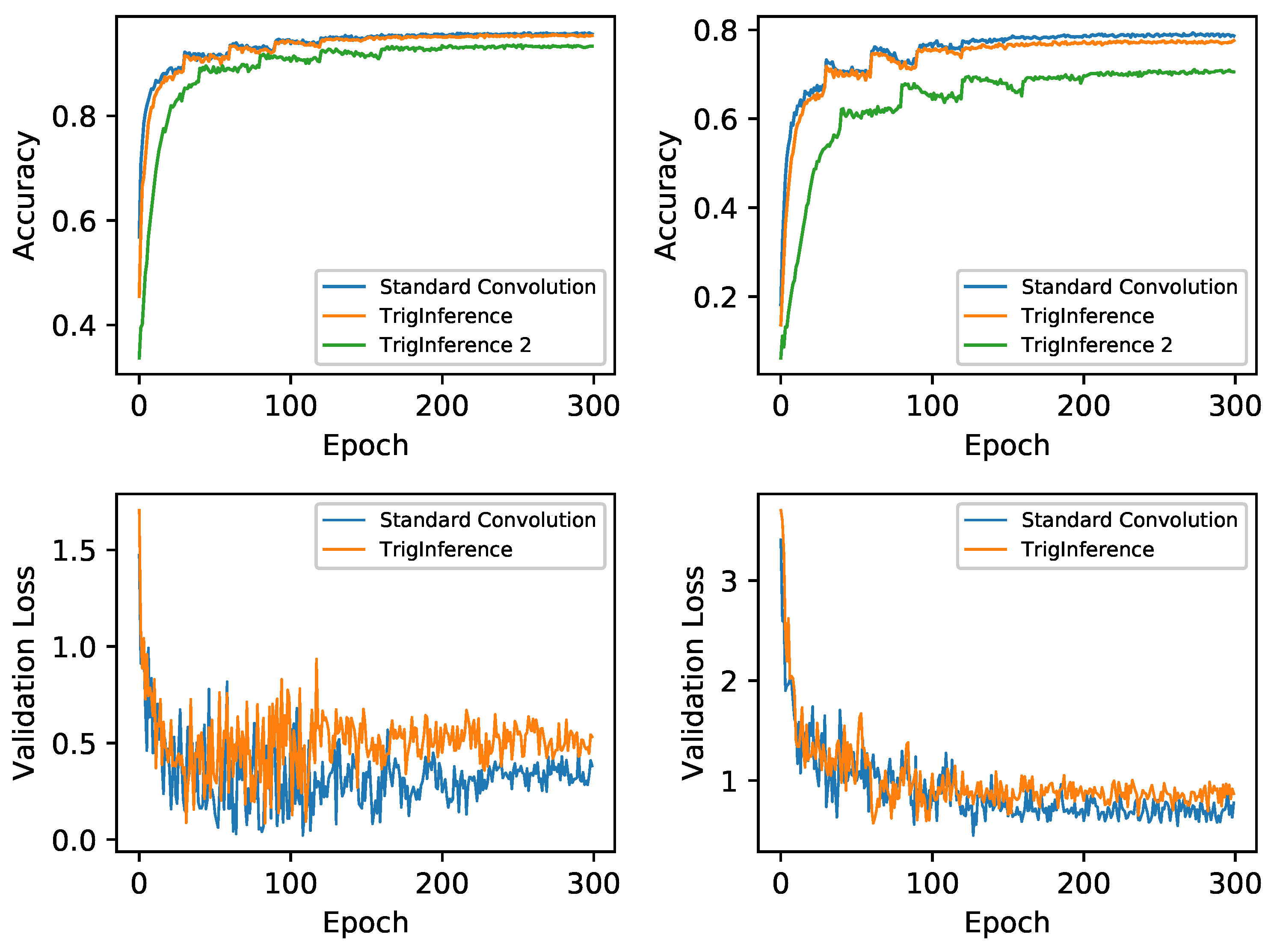
Table 5 summarizes the classification results on two datasets. The training accuracy and loss curves of WideResNet are illustrated in Figure 5. As Figure 5 implies, trigonometric inference provides a close performance to standard convolution counterparts on both CIFAR-10 and CIFAR-100. TriInf 1, which calculates more precise error signals, achieves a higher accuracy and the final results decrease by approximately 1%. Although the accuracy deteriorates by approximately 8% on CIFAR-100, coarse error signals (TrigInf 2) are still recommended on simple tasks because a similar performance is provided on CIFAR-10 and the computations are easier.
Table 5.
Final validation accuracy of CIFAR-10 and CIFAR-100.
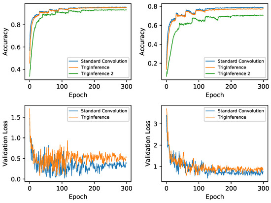
Figure 5.
Training curves of WideResNet on CIFAR-10 and CIFAR-100. The left subplots denote the validation accuracy and loss records on CIFAR-10 and the right subplots denote those on CIFAR-100.
4.3. Narrowing the Accuracy Loss
As Equation (17) indicates, the approximation error of trigonometric inference is upper bounded by: Where x denotes layer inputs and W weights. This approximation error is negligible if the norm between x and W is less than 1. Although most weights and activations in DNNs are very small, there are still a few large ones that affect the final performance. For conventional CNNs the mean of BatchNorm layer is usually set to 1, which is problematic for trigonometric inference since it will bring larger approximation errors. A simple trick to compensate for the accuracy loss is the enforcement of small activations in the batch normalization layers, which introduces no extra computation burdens. To demonstrate this, we did experiments to observe the effect of the mean parameter of batch normalization layers.
We trained ResNet50 models on Cifar-100 dataset, and Momentum SGD was used for gradient descent. For the conventional CNN, we set the mean of BN layers to the default value 1. For TrigInf models, the mean values of BN layers are set to 0.1, 0.5, and 0.7, respectively. We trained each model for 200 epochs (with learning rate decayed to half at (60, 100, 140, 180) epochs) and the results are summarized in Table 6. We can clearly see that the same accuracy and validation loss as the baseline CNN can be obtained by reducing the mean parameter of BN layers.
Table 6.
Evaluation results on Cifar-100 with BN layers’ mean set to different values.
4.4. Compatibility with Other Optimizers
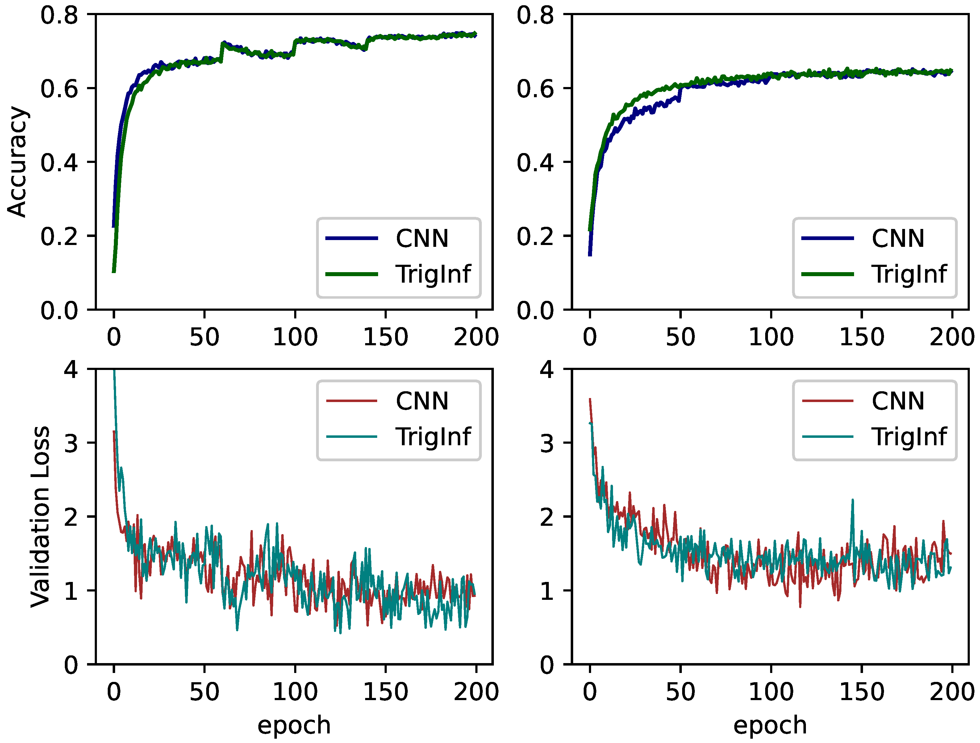
The trigonometric inference is compatible with other gradient descent optimizers such as AdaDelta, Adam, Nesterov Accelerated Gradient (NesterovAG), etc. To show this, we evaluated trigonometric inference on different gradient descent optimizers. Apart from SGD, we tested Adam and NesterovAG with ResNet50 and GoogleNet on Cifar-100, respectively. Figure 6 demonstrates the training curves and validation loss descent curves. As illustrated in Figure 6, on both optimizers trigonometric inference can achieve the same accuracy as conventional CNNs.
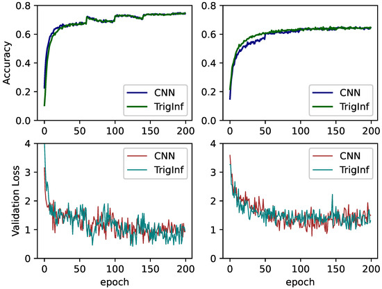
Figure 6.
Training curves and Validation loss of GoogleNet and ResNet5 on CIFAR-100 dataset. The left subplots denote the validation accuracy and loss records on GoogleNet and the right subplots denote those on ResNet50.
5. Future Research and Challenges
To the best of our knowledge, this is the first study to utilize a trigonometric approximation of all parameters in the training of deep neural networks. However, on modern GPUs and CPUs, we were unable to show the efficiency of our training methods because they are specifically optimized for multiplication. We set as our future study the design of a hardware computation engine for trigonometric inference. Here, we briefly discuss the challenges. Although a simple serial CORDIC module requires significantly fewer logic resources than a multiplier, it has certain flaws in terms of speed. To accelerate the CORDIC module for neural network inference, the following two schemes are worth applying:
(1) CORDIC optimization for small values:
Although randomly distributed, layer inputs, weights, and back-propagated errors tend to have small variances in large deep neural networks. Starting the rotation from the mean value can reduce the number of iterations for the CORDIC modules because the mean value can be selected as a pre-computed angle.
(2) Neural network training with lower-precision CORDIC:
As mentioned in Section 2, training with a lower precision can provide a comparable performance under many scenarios. Reducing the model precision to 16-bits, 8-bits, or even fewer bits will significantly decrease the CORDIC iteration times. Therefore, the training efficiency is higher when a lower precision is required.
6. Conclusions
A novel technique for neural network training was introduced in this study. We analyzed the precision of the sine approximation for deep neural network parameters. In addition, we exploited a rectified sine activation function to remove multiplications in inference and training. Trigonometric inference is suitable for scenarios in which the hardware multiplier is insufficient, and is preferred when a hyperbolic activation function is utilized. Our experimental results demonstrate that a comparable performance was achieved using this approach.
The results of this research shed new light on future hardware customization for deep neural networks that aim to take advantage of the CORDIC computation engine and reduce the logic resources and power consumption. It is also practical for applications on weak terminals, such as microcontrollers equipped with CORDIC modules.
Author Contributions
Conceptualization: J.C. and Y.Q. Software: J.C. and M.T. Supervision: H.N. All authors have read and agreed to the published version of the manuscript.
Funding
This research is partly supported by a project, JPNP16007, commissioned by the New Energy and Industrial Technology Development Organization (NEDO) and JSPS KAKENHI, Grant Numbers 21K11804 and 19K11879.
Institutional Review Board Statement
Not applicable.
Informed Consent Statement
Not applicable.
Data Availability Statement
Not applicable.
Conflicts of Interest
The authors declare no conflict of interest.
References
- Volder, J. The CORDIC computing technique. IRE Trans. Electron. Comput. 1959, EC-8, 330–334. [Google Scholar] [CrossRef]
- Tiwari, V.; Khare, N. Hardware implementation of neural network with Sigmoidal activation functions using CORDIC. Microprocess. Microsyst. 2015, 39, 373–381. [Google Scholar] [CrossRef]
- Chen, Y.H.; Chen, S.W.; Wei, M.X. A VLSI Implementation of Independent Component Analysis for Biomedical Signal Separation Using CORDIC Engine. IEEE Trans. Biomed. Circuits Syst. 2020, 14, 373–381. [Google Scholar] [CrossRef]
- Koyuncu, I. Implementation of high speed tangent sigmoid transfer function approximations for artificial neural network applications on FPGA. Adv. Electr. Comput. Eng. 2018, 18, 79–86. [Google Scholar] [CrossRef]
- Shomron, G.; Weiser, U. Spatial correlation and value prediction in convolutional neural networks. IEEE Comput. Archit. Lett. 2018, 18, 10–13. [Google Scholar] [CrossRef] [Green Version]
- Shomron, G.; Banner, R.; Shkolnik, M.; Weiser, U. Thanks for nothing: Predicting zero-valued activations with lightweight convolutional neural networks. In Proceedings of the European Conference on Computer Vision, Glasgow, UK, 23–28 August 2020; pp. 234–250. [Google Scholar]
- Shomron, G.; Weiser, U. Non-blocking simultaneous multithreading: Embracing the resiliency of deep neural networks. In Proceedings of the 2020 53rd Annual IEEE/ACM International Symposium on Microarchitecture (MICRO), Athens, Greece, 17–21 October 2020; pp. 256–269. [Google Scholar]
- Cai, J.; Takemoto, M.; Nakajo, H. A deep look into logarithmic quantization of model parameters in neural networks. In Proceedings of the 10th International Conference on Advances in Information Technology, Bangkok, Thailand, 10–13 December 2018; pp. 1–8. [Google Scholar]
- Sanyal, A.; Beerel, P.A.; Chugg, K.M. Neural Network Training with Approximate Logarithmic Computations. In Proceedings of the ICASSP 2020 IEEE International Conference on Acoustics, Speech and Signal Processing, Barcelona, Spain, 4–8 May 2020; pp. 3122–3126. [Google Scholar]
- Nair, V.; Hinton, G.E. Rectified linear units improve restricted boltzmann machines. In Proceedings of the 27th International Conference on Machine Learning (ICML-10), Haifa, Israel, 21–24 June 2010; pp. 807–814. [Google Scholar]
- Hubara, I.; Courbariaux, M.; Soudry, D.; El-Yaniv, R.; Bengio, Y. Binarized neural networks. Adv. Neural Inf. Process. Syst. 2016, 29, 4107–4115. [Google Scholar]
- Rastegari, M.; Ordonez, V.; Redmon, J.; Farhadi, A. Xnor-net: Imagenet classification using binary convolutional neural networks. In Proceedings of the European Conference on Computer Vision, Amsterdam, The Netherlands, 8–16 October 2016; pp. 525–542. [Google Scholar]
- Banner, R.; Hubara, I.; Hoffer, E.; Soudry, D. Scalable methods for 8-bit training of neural networks. arXiv 2018, arXiv:1805.11046. [Google Scholar]
- Bhandare, A.; Sripathi, V.; Karkada, D.; Menon, V.; Choi, S.; Datta, K.; Saletore, V. Efficient 8-bit quantization of transformer neural machine language translation model. arXiv 2019, arXiv:1906.00532. [Google Scholar]
- Shomron, G.; Gabbay, F.; Kurzum, S.; Weiser, U. Post-Training Sparsity-Aware Quantization. arXiv 2021, arXiv:2105.11010. [Google Scholar]
- Chen, H.; Wang, Y.; Xu, C.; Shi, B.; Xu, C.; Tian, Q.; Xu, C. AdderNet: Do We Really Need Multiplications in Deep Learning? arXiv 2019, arXiv:1912.13200. [Google Scholar]
- Miyashita, D.; Lee, H.E.; Murmann, B. Convolutional Neural Networks using Logarithmic Data Representation. arXiv 2016, arXiv:1603.01025. [Google Scholar]
- Elhoushi, M.; Shafiq, F.; Tian, Y.; Li, J.Y.; Chen, Z. DeepShift: Towards Multiplication-Less Neural Networks. arXiv 2019, arXiv:1905.13298. [Google Scholar]
- Jaime, F.J.; Sánchez, M.A.; Hormigo, J.; Villalba, J.; Zapata, E.L. Enhanced scaling-free CORDIC. IEEE Trans. Circuits Syst. I Regul. Pap. 2010, 57, 1654–1662. [Google Scholar] [CrossRef]
- Mokhtar, A.; Reaz, M.; Chellappan, K.; Ali, M.M. Scaling free CORDIC algorithm implementation of sine and cosine function. In Proceedings of the World Congress on Engineering (WCE’13), London, UK, 3–5 July 2013; Volume 2. [Google Scholar]
- Chen, K.T.; Fan, K.; Han, X.; Baba, T. A CORDIC algorithm with improved rotation strategy for embedded applications. J. Ind. Intell. Inf. 2015, 3, 274–279. [Google Scholar] [CrossRef]
- Tiwari, V.; Mishra, A. Neural network-based hardware classifier using CORDIC algorithm. Mod. Phys. Lett. B 2020, 34, 2050161. [Google Scholar] [CrossRef]
- Heidarpur, M.; Ahmadi, A.; Ahmadi, M.; Azghadi, M.R. CORDIC-SNN: On-FPGA STDP Learning with Izhikevich Neurons. IEEE Trans. Circuits Syst. I Regul. Pap. 2019, 66, 2651–2661. [Google Scholar] [CrossRef]
- Hao, X.; Yang, S.; Wang, J.; Deng, B.; Wei, X.; Yi, G. Efficient Implementation of Cerebellar Purkinje Cell with CORDIC Algorithm on LaCSNN. Front. Neurosci. 2019, 13, 1078. [Google Scholar] [CrossRef] [PubMed] [Green Version]
- Sopena, J.M.; Romero, E.; Alquezar, R. Neural networks with periodic and monotonic activation functions: A comparative study in classification problems. In Proceedings of the 9th International Conference on Artificial Neural Networks, Edinburgh, UK, 7–10 September 1999; pp. 323–328. [Google Scholar]
- Parascandolo, G.; Huttunen, H.; Virtanen, T. Taming the Waves: Sine as Activation Function in Deep Neural Networks. 2016. Available online: https://openreview.net/pdf?id=Sks3zF9eg (accessed on 18 July 2021).
- Ramachandran, P.; Zoph, B.; Le, Q.V. Searching for activation functions. arXiv 2017, arXiv:1710.05941. [Google Scholar]
- Zhang, Y.; Qu, L.; Liu, J.; Guo, D.; Li, M. Sine neural network (SNN) with double-stage weights and structure determination (DS-WASD). Soft Comput. 2016, 20, 211–221. [Google Scholar] [CrossRef]
- Lillicrap, T.P.; Cownden, D.; Tweed, D.B.; Akerman, C.J. Random synaptic feedback weights support error backpropagation for deep learning. Nat. Commun. 2016, 7, 13276. [Google Scholar] [CrossRef]
- Crafton, B.A.; Parihar, A.; Gebhardt, E.; Raychowdhury, A. Direct feedback alignment with sparse connections for local learning. Front. Neurosci. 2019, 13, 525. [Google Scholar] [CrossRef]
- Nøkland, A. Direct feedback alignment provides learning in deep neural networks. arXiv 2016, arXiv:1609.01596. [Google Scholar]
- Heidarpour, M.; Ahmadi, A.; Rashidzadeh, R. A CORDIC based digital hardware for adaptive exponential integrate and fire neuron. IEEE Trans. Circuits Syst. I Regul. Pap. 2016, 63, 1986–1996. [Google Scholar] [CrossRef]
- Chetlur, S.; Woolley, C.; Vandermersch, P.; Cohen, J.; Tran, J.; Catanzaro, B.; Shelhamer, E. cudnn: Efficient primitives for deep learning. arXiv 2014, arXiv:1410.0759. [Google Scholar]
- Tokui, S.; Oono, K.; Hido, S.; Clayton, J. Chainer: A next-generation open source framework for deep learning. In Proceedings of the Workshop on Machine Learning Systems (LearningSys) in the Twenty-Ninth Annual Conference on Neural Information Processing Systems (NIPS), Montreal, QC, Canada, 7–12 October 2015; Volume 5, pp. 1–6. [Google Scholar]
- Simonyan, K.; Zisserman, A. Very deep convolutional networks for large-scale image recognition. arXiv 2014, arXiv:1409.1556. [Google Scholar]
- Zagoruyko, S.; Komodakis, N. Wide residual networks. arXiv 2016, arXiv:1605.07146. [Google Scholar]


Publisher’s Note: MDPI stays neutral with regard to jurisdictional claims in published maps and institutional affiliations. |
© 2021 by the authors. Licensee MDPI, Basel, Switzerland. This article is an open access article distributed under the terms and conditions of the Creative Commons Attribution (CC BY) license (https://creativecommons.org/licenses/by/4.0/).