Inferring Long-Term Demand of Newly Established Stations for Expansion Areas in Bike Sharing System

Abstract

Research on flourishing public bike-sharing systems has been widely discussed in recent years. In these studies, many existing works focus on accurately predicting individual stations in a short time. This work, therefore, aims to predict long-term bike rental/drop-off demands at given bike station locations in the expansion areas. The real-world bike stations are mainly built-in batches for expansion areas. To address the problem, we propose LDA (Long-Term Demand Advisor), a framework to estimate the long-term characteristics of newly established stations. In LDA, several engineering strategies are proposed to extract discriminative and representative features for long-term demands. Moreover, for original and newly established stations, we propose several feature extraction methods and an algorithm to model the correlations between urban dynamics and long-term demands. Our work is the first to address the long-term demand of new stations, providing the government with a tool to pre-evaluate the bike flow of new stations before deployment; this can avoid wasting resources such as personnel expense or budget. We evaluate real-world data from New York City’s bike-sharing system, and show that our LDA framework outperforms baseline approaches.

1. Introduction

A prominent sharing economy business model, the bike-sharing systems, has emerged in recent years as a popular way of public transportation [1]. For society, a bike-sharing system meets the theme of sustainable development because of convenience, lower prices, and environmental protection [2,3]. Consequently, many bike-sharing systems are being established to satisfy the need. One example of a bike-sharing system is Citi Bikes, with more than 85,000 active users [4].

Distributing a suitable bicycle network structure can not only connect the system of urban traffic and commuting but reduce the greenhouse effect. However, constructing unwanted stations in a bike-sharing system will cause environmental damage and resource waste. The framework presented in the paper aims to assist the government and planners in predicting bike demands at a macroscopic level in advance, i.e., evaluating and verifying whether new stations meet the needs of the public.

Research on bike-sharing systems has been widely studied in recent years. Some works [5,6,7,8] depend completely on station-based historical records and features, and their target is to make predictions for already established stations. The works of [9,10] aim to predict the demand in hours or only during rush hour. The work of [11] defines functional zones [12,13] and then predicts that the demand for bike expansion is the most relevant one to our work. Unfortunately, their mobility trip data in the expanded system is inapplicable for our long-term scenario, as it is also regarded as future data in the prediction stage. Different from previous works, we commit to long-term demand prediction, which is faced with two challenges. First, mobility and meteorology data used in previous works are unavailable in expansion areas, for example, taxi usages, temperature, wind speed, etc. Moreover, we cannot directly apply the methodology of existing works, which focus on short-term demand prediction for a single station, since they usually have enough training data but lack future events [5]. Second, the real-world bike stations are mainly built-in batches for expansion areas. However, the different geographical characteristics between regions make the prediction task hard.

To tackle these challenges, we propose a robust framework called LDA (Long-Term Demand Advisor) to predict long-term (e.g., six months) demand in newly established bike regions. Apart from the short-term prediction, which is highly affected by emergencies and other temporal factors [6,7], the proposed long-term prediction can not only reduce inaccuracies resulted from unpredictable social events or traffic accidents but also advise decision-makers on where to build new stations. This framework aims to provide governments with a preliminary estimation of the amount of bike usages in the following periods (e.g., half-year) in the new regions of a city, given merely the locations of the bike stations. Our contributions are as follows:

• To the best of our knowledge, this is the first work to predict long-term bike demand in batches for expansion areas.
• A G-clustering algorithm, a hierarchical POI clustering method to cluster POI categories, is proposed in this work, and it is shown to be effective. Experiments carried out on real-world datasets prove that our LDA framework outperforms baseline approaches.

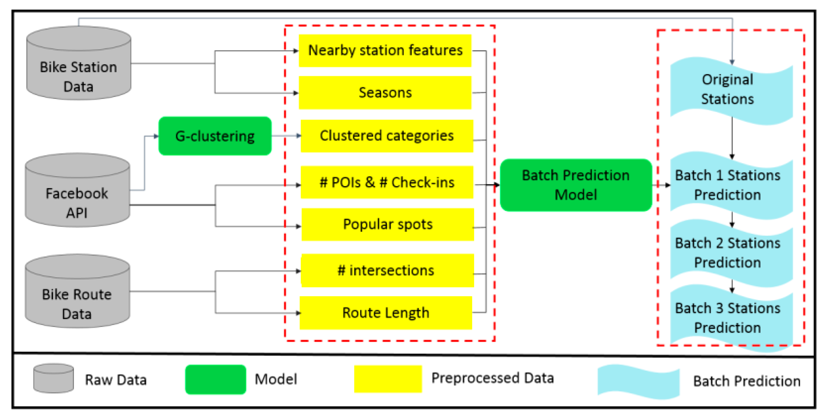
2. Overview

We propose a robust framework called LDA (Long-Term Demand Advisor) to predict long-term (e.g., six months) demand in newly established bike regions. We first extract spatial and temporal features from multi-source open data, then apply our proposed G-clustering algorithm to measure the geographical characteristics and urban correlations in a city. The G-clustering algorithm takes the surrounding locations of the target candidate location into consideration to make a better prediction. Moreover, we extract the urban factors correlated with the long-term demand of sharing bikes, such as POIs (Point of Interests), road structure, and time. On the other hand, features from existing neighbor stations and future stations that have an overlapping operating period are also applied to new bike stations predictions since they will influence the number of demands and transit behaviors.

Our work focuses on long-term prediction, e.g., six months, since the short-term prediction (e.g., one month) is too difficult to predict and not worth studying in practice due to initially unstable environments. Moreover, the long-term effectiveness of stations seems worth investigating to aid in the government’s decision and urban planning. For the reasons above, we consider that the predictions of no less than six months are relatively appropriate for urban decision-making. Figure 1 shows our proposed LDA framework, which consists of two major components: data preprocessing and batch prediction.

Figure 1. The overview of LDA Framework.

Data preprocessing. We first collect government open data and fetch others from Facebook Place API. We also record the latitude and the longitude of all bike stations. Next, we extract spatial features for each station, including nearby station features, seasons, number of POIs and number of check-ins, popular spots, number of intersections, and the length of bike routes based on the parameter r of the reachable station region. Finally, the proposed G-clustering algorithm is applied to cluster categories, and all of the extracted features are prepared to be fed into prediction models. Numerical data normalization, data cleaning, and missing data imputation are also applied to all features.

Batch prediction. We observe that new stations are sometimes constructed in batches in the real world. For example, the bike station deployment of New York from 2013 to 2017 can be mainly divided into four stages. Each stage contains at least 97 stations to be established in a newly expanded area. After data preprocessing, we split stations into original ones and the others in batches according to their month of establishment. From Batch 1 to Batch n (n = 3 for the NYC example) predictions, stations established before the corresponding period are set as training sets, and those in the period are testing sets. Finally, a strong prediction model can be applied to finish n batches of predictions.

3. Methodology

In this section, we introduce (a) our proposed G-clustering algorithm, (b) extracted features correlated with rental/drop-off demand, and (c) demand prediction. We define notations used in this paper in Table 1. Problem definitions and our proposed framework are explained in Section 3.1.

Table 1. Notations used in this paper.

Notations	Descriptions
S	The station set S = {S1, S2, …Sn}
C	The category set C = {CT1, CT2, …CTm}
POI	The POI set POI = {P1, P2, …Pl}
R	The bike route set R = {R1, R2, …Rk}
n, m, l, k	Number of stations/categories/POIs/bike routes
Si	The feature set of ith station
Si·rent	Rental demand for Si six months after the establishment
Si·drop	Drop-off demand for Si six months after the establishment
Si·lat	Latitude of Si
Si·long	Longitude of Si
Si·date	The established date (e.g., operating date) of Si
CS (Si, Sj)	Cosine similarity between Si and Sj
Pl×m	Category matrix corresponding to POIs

3.1. Preliminary and Problem Definition

Definition 1.

Reachable Station Region. Considering how far a resident is willing to move and to get appropriate modeling of spatial factors, we define r as the radius of the farthest influencing area of a new station. In other words, when considering a location to build a new bike station, we propose to set a Euclidean distance r to extract the neighbor characteristics and features. Figure 2 gives an example. S_i is the target location, and we extract the density of our pre-defined POIs, which may be correlated with bike demands within the region.

Figure 2. An illustration of the reachable region of station S_i and the corresponding bike routes.

Definition 2.

Nearby Stations. For the target location of a new station, we extract its top-k nearest stations whose establishment dates are earlier than the corresponding nearby stations. Three features of corresponding nearby stations are considered in our work: the difference of establishment dates, the number of cumulative demands, and the Euclidean distance between the target location and the nearby stations.

Definition 3.

Bike Route Structure. We consider the road length of bike routes and the number of intersections in road structure as features to improve the demand prediction effectiveness. The reason that we consider the road length of bike routes is because a bike station might have a great demand in the long-term if its surrounding environment contains many bike routes, which are convenient for riders to travel by taking bikes. The high number of intersections might also indicate a traffic hub with significant human mobility, leading to increased potential bike flows.

In Figure 3, there are three kinds of bike routes, and a bike route R_i is composed of multiple intersections (red points) and road segments (black dotted lines). Those route segments and intersections within the reachable station region of S_i are needed to be included. That is, the features extracted from R₁, R₂, and partial of R₃ in Figure 2 should be taken into consideration.

Figure 3. Examples of bike route intersection.

Definition 4.

Season. The period after building a station will span multiple seasons, and all of them should be considered since the commuting behavior of people will change with seasons. For each target station, we calculate how many months it will operate in each season. Spring is defined as the months from March to May, and the season changes every three months.

Definition 5.

Category Vector P_i for Each POI. A POI P_i may have more than one corresponding category defined in Facebook Place API. Then, we define P_i as:

P_i = {p_{i, j}}

(1)

where p_i,j = 1, if P_i belongs to CT_j; or 0, otherwise.

Where CT_j is the jth element in the category set defined by Facebook.

Problem Definition.Rental/Drop-off demand prediction. Given k new bike station locations S_N = {S₁, S₂, …, S_k}, we want to predict the rental/drop-off demands of each station six months after its establishment; that is, S_i rent/S_i drop defined in Table 1.

3.2. G-Clustering

Since thousands of corresponding categories for POIs exist in certain regions, it is impractical to perform a one-to-one clustering for mapping a single category to a class. Therefore, we propose G-clustering to allocate categories into classes, where the characteristics of each category are similar to those of all the other categories in the same class. The G-clustering is inspired by the Gini coefficient [14], which is an index proposed by Corrado Gini to judge the fairness of annual income distribution according to the Lorenz curve. In order to apply the concept of the Lorenz Curve in our work, we modify the definition of it, which is illustrated in Figure 4. The Gini coefficient is equal to the area ratio between A and (A + B), and it is also equal to 2A since the sum area of A and B is 0.5.

Figure 4. Lorenz Curve.

We apply this index to evaluate the distribution for each category in several regions clustered by geographical locations in the given problem space, and thus categories with similar distribution into the same clusters. The pseudocode for the G-clustering algorithm is depicted in Algorithm 1.

Algorithm 1 G-Clustering Algorithm

Input:  C,  POI, $\mathit{P}$; Output:$\mathit{C}{\mathit{C}}^{\mathit{D}}$; 1.  Cluster POI into $D_1$ clusters: $C_1,C_2,C_3\dots C_{D_1}$ by DBSCAN according to POI geographical locations; 2.  Initialize ${\mathit{H}}^{\mathit{D}}=0$; 3.  for i = 1 : $m$ do 4.      for j = 1: $l$ do 5.         if $p_{j,i}$ == 1 then 6.       $h_{i,C_d}$+= 1; 7.  end for 8.  Initialize $\mathit{C}{\mathit{C}}^{\mathit{D}}=\left\{\mathit{C}{\mathit{C}}_{\mathbf{0}}, \mathit{C}{\mathit{C}}_{\mathbf{1}},\dots \mathit{C}{\mathit{C}}_{\mathit{l}}\right\}$; 9.  for k = 1: m do 10.    Category_point = CVF ($h_k$); 11.    idx = [10* Category_point] − 2; 12.   $\mathit{C}{\mathit{C}}_{\mathit{i}\mathit{d}\mathit{x}}$ append category k; 13. end for 14. function CVF (array A) 15.    A_norm = normalized(A); 16.    category_value_point = (1 − gini(A_norm)) + $\frac{\mathrm{gini}\left(A\_norm\right)}{{\log }_{10}(sum\left(A\_norm\right))+1}$; 17. return category_value_point

The proposed G-clustering is composed of three parts: initialization (line 1), construction for heat matrix (line 2 to 7), clustering for categories (line 8 to 13). First, POI is clustered into $D_1$ clusters, where $D_1$ is adjustable and set to 20 in our evaluation. Next, a heat matrix ${\mathit{H}}^{\mathit{D}}=\left\{h_{i,j}\right\}$ is constructed with $h_{i,j}$ representing the number of the $i\mathrm{th}$ category in the $j\mathrm{th}$ cluster according to $\mathit{P}$. Meanwhile, $C_d$ refers to the corresponding cluster result of the $j\mathrm{th}$ POI in line 1. We divide each category into different groups according to its value point; the result $\mathit{C}{\mathit{C}}^{\mathit{D}}$ is returned once all categories are run through and assigned to a certain cluster. Each item in $\mathit{C}{\mathit{C}}^{\mathit{D}}$ indicates a set of the same level categories; meanwhile, we set $l$ = 6 in the following evaluation.

Line 14 to 17 is a function that calculates the category value point. In this function, the Gini coefficient is applied to measure the distribution of each category in different clusters. The more even the distribution is, the closer this index gets to 0 (closer to the blue line in Figure 4); otherwise, it gets closer to 1 (closer to the red line in Figure 4). The function in lines 14 to 17 is designed to determine whether a category is indicative or not. The more even the distribution, the higher the value point, and the less indicative the category is. On the other hand, we also apply K-means to reallocate POI into $D_2$ clusters as described in line 1, where $D_2$ is set to 20 in our evaluation, and all other steps for G-clustering are left the same. The two types of clustering results are listed in Table 2.

Table 2. Results of G-clustering.

	POI Categories
	DBSCAN	K-Means
Cluster 1	Reptile Per Store, Boat/Sailing, Instructor, Night Market	Archery Shop, Night Market, Squash Court
Cluster 2	Art Gallery, Local Business, Arts and Entertainment	Consulate and Embassy
Cluster 3	Elementary School, Language School, Lawyer and Law Firm	Art Gallery, Airport Lounge, Airport Terminal, Cruise Line
Cluster 4	Travel Service, Video Game, Junior High School, Public Swimming Pool	Surfing Spot, Landmark and Historical Place, College and University
Cluster 5	Music Video, Skate Shop, Football Stadium Education Company	Junior High School, Lawyer and Law Firm, Taxi Service
Cluster 6	Aquarium, Diagnostic Center, Drive-In Movie Theater	Public Swimming Pool, Bus Station, Supermarket, Pizza Place
Cluster 7	Fitness Venue, Hockey Arena, Retail Bank	Gas Station, Catholic Church

We list several representative categories in each cluster to explain the effectiveness of the G-Clustering algorithm. In the left column of Table 2 (DBSCAN), categories more evenly distributed in the area such as Fitness Venues and Retail Banks are clustered in the same class since these types of POIs have no obvious regional characteristics. In other words, there is no excessive demand from these categories in specific districts. On the contrary, the number of Night Markets and Art Galleries is obviously larger in certain areas and thus may be regarded as indicative categories in the prediction. A similar trend can also be found in the right column of Table 2 (K-means). The small difference between DBSCAB and K-means clustering results in some categories being clustered in different hierarchies. For example, Art Galleries and Junior High Schools are in different clusters, which might be due to their different local characteristics. The clustering results will then be used as important categorical features for the bike stations.

3.3. Feature Extraction

We divide all features into six categories based on their data sources. They are I.#POI and #Checkins, II. Nearby station features, III. Popular spots, IV. G-clustering, V. Bike route structure, VI. Season. In the experiment, we will evaluate the effectiveness of these six categories. In Table 3, we give an overview of features.

Table 3. All Features and their Descriptions.

Features
Feature Name	Description
POIs	#POIs in Facebook
check-ins	# check-ins in Facebook
Nearby station features	The difference of establishing dates, the number of cumulative demands, and the Euclidean distance between the target location and their nearby stations
G-clustering (DBSCAN)	Category clustering results by applying DBSCAN
G-clustering(K-means)	Category clustering results by applying K-means
Bike route structure	Sum of total route length and the number of intersections of bike routes in the reachable region of the station
Season	Operating seasons

I. #POI and #Checkins. The number of POIs (Point-Of-Interests) and check-ins can be indicated as the level of prosperity in an area and therefore results in a higher frequency of bike demands. We extract #POI and #Checkin’s based on Facebook API.

II. Nearby station features. A new station is usually highly related to the nearby stations due to spatial effect and human mobility. Three features of top-k nearby stations are considered in our work: the difference in establishing dates, the number of cumulative demands, and the Euclidean distance between the target location and their nearby stations. If a nearby station is built later than the target location, the number of cumulative demands will be set as zero. After extraction, we obtain a total of 3 k features for nearby stations. Such a large number might dominate the prediction result of the classifier. Therefore, PCA (Principal Component Analysis) is applied to reduce feature dimensions.

III. Popular spots. We define popular types of POIs (e.g., over 1000 stores in New York) specifically, calculating the number of corresponding types of POIs and check-ins of each station in its reachable station region.

IV. G-clustering. We perform the G-clustering algorithm to use the clustering result as our features. We set two kinds of clustering methods in step 1 of G-clustering: one is DBSCAN, and the other is K-means.

IV-D. Category clustering results applying DBSCAN.

IV-K. Category clustering results applying K-means.

V. Bike route structure. The more bike routes near a station, the higher the probability the bikes will be rented for convenience. We then calculate the sum of total route length and the number of intersections of bike routes in the reachable region of station $S_i$.

VI. Season. Seasons will greatly affect people’s willingness to ride a bike. For example, users tend to rent a bike in spring rather than in winter, so data in December is obviously less than in May. According to Definition 4, if station $S_i$starts operating in May, then the number of months in the following six months from spring to winter is 1, 3, 2, 0.

3.4. Batches Prediction

Constructing a bike-sharing system in most cities can be realized in several steps (batches). First, the government sets up a large number of bike station locations in the downtown area where lots of commercial buildings and tourist attractions are located, spreading out to nearby regions in the following months, perhaps with a short lull. However, as the frequency of shared bikes and new users increases, the government needs to distribute a wider range of bike locations to satisfy users’ demand, and therefore the area expands to the suburbs and even empty districts in the city center to relieve excessive demand.

Definition 6.

Batches Prediction. Our work focuses on batch prediction; in other words, site prediction established in later stages in the suburbs or border zones, which are also defined as expansion areas in this paper. We propose to utilize EMA (Exponential Moving Average) to determine the periods of batches given a continuous time interval. The EMA is a type of average that applies weighting factors that decrease exponentially to the past. We define a batch that exists if the EMA values of month demands are continuously not less than a given threshold for several months. Figure 5 shows the EMA distribution that we perform using 2, 3, and 6 months as the average units. For example, if we define the threshold as 30 using the two months average of EMA for New York City, we can then identify three batches(peaks) from 2013 to 2018. The corresponding periods of the first, second and third batches of NYC are shown in Table 4. Our framework provides the government the estimation of the demands of newly established stations through given locations, and this can also be applied to the expansion of other facilities.

Figure 5. EMA of each month.

Table 4. Data source and detailed contents.

	New York Citi Bike System
Time Span	Origin	Batch 1	Batch 2	Batch 3
	June 2013~June 2015	August 2015~September 2015	August 2016~September 2016	September 2017~October 2017
# Stations	329	121	127	97
	Facebook Place API
# Check-ins	175+ billion
# POI Categories	1279
	New York Bike Route
# Intersections	26,868
Total Length	1300+ km

In this work, we mainly use XGBoost [15] to make the prediction for each batch. Apart from XGBoost in this work, other machine learning approaches can also be applied under our framework. We will compare their effectiveness in our experiments.

4. Experiments

To evaluate the performance of our framework, we conduct experiments on a real-world dataset from New York Citi Bike. Details of multi-source open data are in Table 4. Bike station data are collected from June 2013 to November 2018, and stations operating for less than six months, or with a monthly average demand of less than 300, are removed. Batches can be realized as the time period of a relatively large number of bike stations construction. Stations with established dates from June 2013 to July 2015 are the origin. From Batch 1 to 3 prediction, we divide stations in the training set and testing set according to their established date. For instance, in Batch 2 prediction, stations established earlier than August 2016 are training data, and the other stations established during August 2016 to September 2016 are testing data. We retrieve multi-source open data from Citi Bike (the bike-sharing system in New York), bike routes data, and Facebook Place API. Detailed datasets are listed in Table 4. The settings for radius r of the reachable station region are 500 m, and we extract the top-15 nearby station features in our experiment.

4.1. Experimental Settings

We evaluate the effectiveness of different combinations of feature sets, which are listed in Table 5. A single factor is not listed due to the low performance; however, important factors such as I and II are included in each set.

Table 5. Feature set combination.

Feature Set	Features
	I + II	III	IV-D	IV-K	V	VI
A	■		■
B	■				■
C	■	■	■			■
D	■			■	■
E	■	■			■	■
F	■	■	■		■	■
G	■	■		■	■	■
CC-XGB	■	■	■	■	■	■

4.1.1. Baselines

The framework proposed in our work is denoted as Category Clustering applying eXtremeGradient Boosting (CC-XGB). XGBoost [15] is regarded as one of the most powerful techniques in the public transportation domain.

Regressors such as RF (Random Forest), LR (Linear Regression), and SVR (Support Vector Regression) are used in comparison; NN (Neural Network) is also included as a predictor. Moreover, the following compared baselines according to historical average demand are used to verify the performance of our models.

HA (History Average). History rental/drop-off average of stations whose established months are earlier than the predicted station $S_i$.

HSA (History Similarity Average). History rental/drop-off average of stations whose established month is earlier and is in the top-five high cosine similarity with the predicted station $S_i$.

HSW (History Similarity Weight). Let $S_{i,1}~S_{i,5}$ be the top-five high cosine similarity stations to the predicted station $S_i$.

$$\mathrm{HSW}\left(S_i\right)=\frac{{\sum }_{k=1}^5\left(S_i·rent\right)\ast CS\left(S_i,S_{i,k}\right)}{{\sum }_{k=1}^{5}CS\left(S_i,S_{i,k}\right)}$$

(2)

HSC (History in the Same Cluster). History rental/drop-off average of stations whose established months are earlier in the same DBSCAN cluster with station $S_i$.

HNN (History Nearest Neighbors). History rental/drop-off average of stations whose established month is earlier and distance in the top-k nearest with the predicted station $S_i$.

4.1.2. Evaluation Metric

Since bike demands vary dramatically due to many factors, RMSLE (Root Mean Squared Logarithmic Error) is a more appropriate metric to adopt.

$$\sqrt{\frac{1}{N}{\displaystyle \sum }_{i=1}^N{\left(\log \left((S_i·rent/drop\right)-\left(\log \left((S_i·{rent}^{\prime }/{drop}^{\prime }\right)\right)\right)}^2}$$

(3)

$S_i·rent/drop$ is the ground truth of demand in six months of $S_i$, and $S_i·{rent}^{\prime }/{drop}^{\prime }$ is the corresponding prediction result of the ground truth.

4.2. Batch Prediction Results

4.2.1. Overall Comparison

In this part, we show the effectiveness of the proposed LDA and the comparison to the baselines.

Results of Baselines: Figure 6a,b represent the baseline results of rental and drop-off, respectively. Baselines without machine learning such as HA, HSA, and HSW are worse than regression or NN results. CC-XGB, our proposed framework, defeats the second-best with an average of 0.2 to 0.3 approximately in RMSLE, whether in a rental or drop-off situation.

Figure 6. Performance of baselines. (a) represents the rental demand and (b) represents the drop-off one.

Results of Feature Combination: Figure 7a,b represent the results of the different combinations of features in rental and drop-off, respectively. The result of feature set E without features of category clustering in Figure 7b has poor performance evidently, confirming that G-clustering is effective. No one always performs better between IV-D and IV-K; one reason may be due to slight differences in clustering results. Though the differences in the batches are not obvious, CC-XGB performs much better than other feature sets in batch 2 and 3, confirming the applicability of our framework.

Figure 7. Performance of different feature combinations. (a) represents the rental demand and (b) represents the drop-off one.

Analyze for Batches: Under the prediction result of CC-XGB, our proposed framework, RMSLE decreases from Batch 1 to 3 in drop-off mode; yet results in Batch 3 are worse than in Batch 2 in rental mode. We infer that the demand for renting bikes downtown is more stable than in other areas; in other words, users are less willing to rent a bike from newly established stations, making the prediction difficult. On the other hand, the drop-off demand is hard to predict for the first batch stations.

4.2.2. Region Size Setting for Extracted Features

In our experiment, the reachable station region is set as 500 m (Figure 1 (left)) for the appropriate number of POIs and check-ins. In this part, we would like to compare how different radiuses affect the results. Features I, III, and V are related to the reachable station number. Experiments are conducted from 300 m to 1000 m in Figure 8. As shown in Figure 8, a larger radius does not necessarily mean a better prediction result. We can observe that in Figure 8, 500 m is a superior radius region for a target station to extract corresponding features since the RMSLE for three batches are relatively low when r = 500 m.

Figure 8. Results of different regions for feature extraction in (a) Rental and (b) Drop-off.

4.2.3. Feature Importance (FI)

Figure 9, Figure 10 and Figure 11 show the feature importance for Batch 1 to Batch 3, and the detailed features whose importance is ranked in the top five are listed aside. Figure 9a, Figure 10a, and Figure 11a show rental feature importance, while Figure 9b, Figure 10b, and Figure 11b show drop-off feature importance. Overall, the nearby station features are extremely important in prediction since they have the highest scores in all situations; in particular, the score gap is more significant in Batch 3 (Figure 11a,b), explaining that nearby stations are highly correlated to newly established stations. The feature importance obtained from G-clustering is all ranked in the top five in those five figures (top-6 in Figure 11a), proving that our idea of clustering categories is reasonable and useful.

Figure 9. Feature importance of Batch 1. (a) Represents rental demand, and (b) represents the drop-off one.

Figure 10. Feature importance of Batch 2. (a) Represents rental demand, and (b) represents the drop-off one.

Figure 11. Feature importance of Batch 3. (a) Represents rental demand, and (b) represents the drop-off one.

4.2.4. Prediction of Different Periods

Our work focuses on long-term prediction, e.g., six months, since the short-term prediction (e.g., one month) is too difficult to predict and not worth studying in practice due to initially unstable environments. The experiments conducted on one, three, six and nine month(s) in Figure 12 and Figure 13 have shown that the six months’ prediction has the best performance. The nine months case is worse than the six months. The reason comes from the data instead of our model. In our dataset, we observe that there are some new stations built surrounding the existing stations after six months so that the demands of some stations in a certain batch were influenced by new stations. The prediction then would become not so accurate. For batch 1, batch 2, and batch 3, the RMSLE of six months is the lowest comparing to one month, three months, and nine months. In batch 1, the gap between six-month and others for rental is from 0.02 to 0.31, and the gap for drop-off is from 0.07 to 0.36. In batch 2, the gap between six-month and others for rental is from 0.07 to 0.2, and the gap for drop-off is from 0.01 to 0.11. In batch 3, the gap between six-month and others for rental is from 0.09 to 0.2, and the gap for drop-off is from 0.03 to 0.09.

Figure 12. Different periods of prediction for Rental.

Figure 13. Different periods of prediction for Drop-off.

4.3. Random Prediction Results

Similar to works focusing on predicting demand through splitting data into the training set and testing set without considering established time, we also repeat the same steps in our experiment to verify the usefulness of our LDA framework. In other words, we conduct the prediction experiment of rental/drop-off demand 10,000 times through randomly divided stations and return the average RMSLE result (Figure 14). The result of CC-XGB still performs the best. However, our superiority is not so apparent since our proposed features are relatively suitable for batch prediction rather than random prediction.

Figure 14. Random prediction for rental/drop-off.

5. Discussion of the Results

In this research, we are facing the demand prediction problem of real-world bike-sharing systems. In the previous experiments, we can observe that two important factors in LDA settings are worth discussing, considering real-world applications. One is batch deployment. Another is the prediction time period. These two factors are mutually high-correlated.

Discussion of batch deployment: In the past, existing works usually aimed to predict human flows for each individual station in a short time, such as next hour, next day, and next 1–3 days. However, in real-world applications, we claim that predicting long-term demands for station deployment is also critical for urban planning and construction. Therefore, we propose an LDA framework, which can help governments or transportation companies to make decisions for deploying bike-sharing services in a smart city. We have observed that the real-world bike stations are mainly built-in batches for expansion areas in modern cities. That is, we can use only the historical demand data from previously deployed areas for prediction. The batch consideration in the LDA framework confirms that our work is the first to address the long-term demand of new stations for future batch stations, providing the government with a tool to pre-evaluate the bike flow of new stations before deployment. LDA can avoid wasting resources such as personnel expense or budget.

Discussion of prediction periods: In Section 4.2.4, our experiment shows that the six months’ prediction has the best performance. The reason is we observe that in the New York Citi bike sharing system there are some new stations built surrounding the existing stations after six months so that the demands of some stations in a certain batch were influenced by new stations. However, we believe our proposed LDA framework is also helpful for making decisions using the prediction results of periods that are more than six months since the prediction error is mainly from the crawled future data. To conclude, our LDA framework can work as a web service to assess the effectiveness of new bike stations for expansion areas in different cities.

6. Related Work

Impacts of bike-sharingsystems. Many studies analyzed the impact of bike-sharing systems on different aspects of society. The work of [16] mentioned that bike-sharing programs have significantly positive externalities, including the economy, the environment, and health-related externalities. Moreover, introducing bike-sharing systems gives an opportunity to organize public transport interchanges better [17]. Shared bicycles facilitate allow getting to stops and stations for those who do not own a private bike. Additionally, bike-sharing gives more flexibility–shared bicycles users are not burdened with the threat of theft or an obligation to service the bicycle. The study of [18] developed a spatial Agent-based model to simulate the use of bike-sharing services and other transport modes in Taipei city. The simulation results indicate that free use of bike-sharing to connect the transit system can be more sustainable with 1.5 million US dollars in transportation damage cost saved per year and 22 premature deaths further prevented per year due to mode shift to cycling and walking based on the business. The work of [19] demonstrated the importance of user-interface (UI) design, social influence, and new media in affecting users’ awareness of and attitude towards uncivilized behaviors, which in turn improve their intention of bike-sharing services use.

The emergence of dockless bike-sharing services has revolutionized bike-sharing markets in recent years. The work of [20] suggested that the dockless design of bike-sharing systems significantly improves users’ experiences at the end of their bike trips. However, the availability and usage rates of dockless bike-sharing systems imply that they may seriously affect individuals’ subjective well-being by influencing their satisfaction with their travel experiences, health, and social participation, which requires further exploration. The work of [21] mentioned that, as Chinese enterprises already invest heavily in Europe, it is crucial for policymakers to introduce rules that would counteract potentially negative consequences of the introduction of a new system of bike-sharing and support positive effects.

Behavior analysis in bike-sharing systems. The behavior patterns of users in bike-sharing systems are also worth exploring. The estimation results of [22] show that descriptive norm, conformity tendency, and past behavior are important factors that affect both e-bike riders’ intention to violate traffic rules and accident proneness. The work of [23] found that perceived ease of use positively influences the attitude towards the systems and the use intention. Therefore, the bike-sharing operating companies should carefully design the usage procedures to make them as simple as possible. The work of [24] adopted machine learning to show that speed, travel distance, and the number of parks and recreational facilities seem to be critical spatial predicting factors of the travel choice in bike-sharing systems. Moreover, considering the impact of COVID-19 on bike-Sharing systems, the work of [25] indicated that usage bike-sharing is more likely to become a more preferable mobility option for people who were previously commuting with private cars as passengers and people who have already registered users in a bike-sharing system. The bike-sharing systems have proved in the study of [26] to be more resilient than the subway system, with a less significant ridership drop and an increase in its trips’ average duration. The work of [27] shows that a high availability rate, a low price, and a large difference in travel time between bike-sharing and other travel modes make potential customers more likely to use a bike-sharing program by modeling a different aspect of travel behavior: heterogeneous time-sensitive customers.

Bike station deployment. Research on bike-sharing systems is becoming more and more prevalent worldwide; topics covered range from site selection to rebalancing bike distribution. The works of [28,29] try to figure out the best locations for bike stations from candidate sites. The work of [30] proposes a mixed model to minimize fixed construction costs and variable operational costs. Research combining probability and simulation such as in [31] develops a probabilistic model to infer future demand, and the work of [32] adopts Monte Carlo to predict the over-demand probability in each bike station cluster. On the other hand, the works of [8,33,34,35] focus on bike imbalance and rebalancing problems, proposing methods to transfer bikes between stations.

Bike demand analysis and prediction. In all bike-related problems, the most widely studied is bike demand or traffic flow prediction. The studies of [22,36] have identified the importance of natural environmental factors such as temperature, precipitation, and humidity on cycling activities across different cities. At the feature level, studies [5,37] consider a single factor instead of multiple aspects features and thus may neglect representative elements. Other works collect historical data such as public transportation pattern records [38], crowd flow [39], meteorology data [7,8,40], and so on. Clustering methods applied to bike stations are more and more common in recent works since bike stations share partially similar regional characteristics and will reduce the variance and improve prediction accuracy. The difference between these works is what the cluster is based on. The works of [7,9,32,41] cluster stations according to bike transition pattern records, geographical locations, bike usage, etc. The study of [42] employs SimRank to calculate the similarities between stations and then adopts the density clustering algorithm OPTICS.

However, the works above are not applicable for our scenario since they rely on the historical mobility data and therefore are unavailable for batch prediction in newly established stations in expansion areas. Furthermore, they mostly aim to predict demand in a relatively short period from hourly [11,43], rush hours [9], to weekends and holidays [32], and thus cannot be applied to our long-term prediction.

7. Conclusions

In this paper, we propose a framework consisting of spatial and temporal features to predict long-term rental/drop-off demand in newly established stations, e.g., in expansion areas. Specifically, we extract features from multi-source open data, propose G-clustering, and apply regression models to predict the demand of stations in three batches according to the established periods. Experiments carried out in the New York Citi bike sharing system demonstrate that our framework for long-term prediction in expansion areas is applicable and outperforms baselines. In the future, we aim to analyze more factors, such as transfer probability from downtown to the suburbs and deal with unusual events to improve predicting accuracy.

References

1. Chen, S.-Y. Using the Sustainable Modified Tam and Tpb to Analyze the Effects of Perceived Green Value on Loyalty to a Public Bike System. Transp. Res. Part A Policy Pract. 2016, 88, 58–72. [Google Scholar] [CrossRef]
2. Cohen, B.; Kietzmann, J. Ride On! Mobility Business Models for the Sharing Economy. Organ. Environ. 2014, 27, 279–296. [Google Scholar] [CrossRef]
3. Eckhardt, G.M.; Bardhi, F. The Sharing Economy Isn’t About Sharing at All. Harv. Bus. Rev. 2015, 28, 881–898. [Google Scholar]
4. Schor, J.B.; Fitzmaurice, C.J. Collaborating and Connecting: The Emergence of the Sharing Economy. Handb. Res. Sustain. Consum. 2015, 26, 410–425. [Google Scholar]
5. Alvarez-Valdes, R.; Belenguer, J.M.; Benavent, E.; Bermudez, J.D.; Muñoz, F.; Vercher, E.; Verdejo, F. Optimizing the level of service quality of a bike-sharing system. Omega 2016, 62, 163–175. [Google Scholar] [CrossRef]
6. Kalvapalli, S.P.K.; Chelliah, M. Analysis and Prediction of City-Scale Transportation System Using XGBOOST Technique. In Recent Developments in Machine Learning and Data Analytics; Springer: Berlin/Heidelberg, Germany, 2019; pp. 341–348. [Google Scholar]
7. Li, Y.; Zheng, Y.; Zhang, H.; Chen, L. Traffic prediction in a bike-sharing system. In Proceedings of the 23rd ACM SIGSPATIAL International Conference on Advances in Geographic Information Systems, Seattle, WA, USA, 3–6 November 2015; pp. 1–10. [Google Scholar]
8. Liu, J.; Sun, L.; Chen, W.; Xiong, H. Rebalancing bike sharing systems: A multi-source data smart optimization. In Proceedings of the 22nd ACM SIGKDD International Conference on Knowledge Discovery and Data Mining, San Francisco, CA, USA, 13–17 August 2016; pp. 1005–1014. [Google Scholar]
9. Feng, Y.; Affonso, R.C.; Zolghadri, M. Analysis of bike sharing system by clustering: The Vélib’case. IFAC-PapersOnLine 2017, 50, 12422–12427. [Google Scholar] [CrossRef]
10. Lin, L.; He, Z.; Peeta, S. Predicting station-level hourly demand in a large-scale bike-sharing network: A graph convolutional neural network approach. Transp. Res. Part C Emerg. Technol. 2018, 97, 258–276. [Google Scholar] [CrossRef] [Green Version]
11. Liu, J.; Sun, L.; Li, Q.; Ming, J.; Liu, Y.; Xiong, H. Functional zone based hierarchical demand prediction for bike system expansion. In Proceedings of the 23rd ACM SIGKDD International Conference on Knowledge Discovery and Data Mining, Halifax, NS, Canada, 13–17 August 2017; pp. 957–966. [Google Scholar]
12. Long, Y.; Shen, Z. Discovering functional zones using bus smart card data and points of interest in Beijing. In Geospatial Analysis to Support Urban Planning in Beijing; Springer: Berlin/Heidelberg, Germany, 2015; pp. 193–217. [Google Scholar]
13. Yuan, N.J.; Zheng, Y.; Xie, X.; Wang, Y.; Zheng, K.; Xiong, H. Discovering urban functional zones using latent activity trajectories. IEEE Trans. Knowl. Data Eng. 2014, 27, 712–725. [Google Scholar] [CrossRef]
14. Gini, C. Measurement of Inequality of Incomes. Econ. J. 1921, 31, 124–126. [Google Scholar] [CrossRef]
15. Chen, T.; Guestrin, C. Xgboost: A scalable tree boosting system. In Proceedings of the 22nd Acmsigkdd, San Francisco, CA, USA, 13–17 August 2016; pp. 785–794. [Google Scholar]
16. Qiu, L.-Y.; He, L.-Y. Bike Sharing and the Economy, the Environment, and Health-Related Externalities. Sustainability 2018, 10, 1145. [Google Scholar] [CrossRef] [Green Version]
17. Brunner, H.; Hirz, M.; Hirshberg, W.; Fallast, K. Evaluation of various means of transport for urban areas. Energy Sustain. Soc. 2018, 8, 9. [Google Scholar] [CrossRef] [Green Version]
18. Lu, M.; Hsu, S.-C.; Chen, P.-C.; Lee, W.-Y. Improving the sustainability of integrated transportation system with bike-sharing: A spatial agent-based approach. Sustain. Cities Soc. 2018, 41, 44–51. [Google Scholar] [CrossRef]
19. Jia, L.; Liu, X.; Liu, Y. Impact of Different Stakeholders of Bike-Sharing Industry on Users’ Intention of Civilized Use of Bike-Sharing. Sustainability 2018, 10, 1437. [Google Scholar] [CrossRef] [Green Version]
20. Chen, Z.; Lierop, D.V.; Ettema, D. Dockless bike-sharing systems: What are the implications? Transp. Rev. 2020, 40, 333–353. [Google Scholar] [CrossRef]
21. Bieliński, T.; Ważna, A. New Generation of Bike-Sharing Systems in China: Lessons for European Cities. J. Manag. Financ. Sci. 2018, 11, 25–42. [Google Scholar]
22. Tang, T.; Guo, Y.; Zhou, X.; Labi, S.; Zhu, S. Understanding electric bike riders’ intention to violate traffic rules and accident proneness in China. Travel Behav. Soc. 2021, 23, 25–38. [Google Scholar] [CrossRef]
23. Yu, Y.; Yi, W.; Feng, Y.; Liu, J. Understanding the Intention to Use Commercial Bike-sharing Systems: An Integration of TAM and TPB. The Sharing Economy. In Proceedings of the 51st Hawaii International Conference on System Sciences, Waikoloa, Big Island, HI, USA, 3–6 January 2018. [Google Scholar]
24. Zhou, X.; Wang, M.; Li, D. Bike-sharing or taxi? Modeling the choices of travel mode in Chicago using machine learning. J. Transp. Geogr. 2019, 79, 102479. [Google Scholar] [CrossRef]
25. Nikiforiadis, A.; Ayfantopoulou, G.; Stamelou, A. Assessing the Impact of COVID-19 on Bike-Sharing Usage: The Case of Thessaloniki, Greece. Sustainability 2020, 12, 8215. [Google Scholar] [CrossRef]
26. Teixeria, J.F.; Lopes, M. The link between bike sharing and subway use during the COVID-19 pandemic: The case-study of New York’s Citi Bike. Transp. Res. Interdiscip. Perspect. 2016, 6, 100166. [Google Scholar] [CrossRef] [PubMed]
27. Chen, Y.; Wang, D.; Chen, K.; Zha, Y.; Bi, G. Optimal pricing and availability strategy of a bike-sharing firm with time-sensitive customers. J. Clean. Prod. 2019, 228, 208–221. [Google Scholar] [CrossRef]
28. Liu, J.; Li, Q.; Qu, M.; Chen, W.; Yang, J.; Xiong, H.; Zhong, H.; Fu, Y. Station site optimization in bike sharing systems. In Proceedings of the 2015 IEEE International Conference on Data Mining, Atlantic City, NJ, USA, 15–17 November 2015; pp. 883–888. [Google Scholar]
29. Martinez, L.M.; Caetano, L.; Eiró, T.; Cruz, F. An optimisation algorithm to establish the location of stations of a mixed fleet biking system: An application to the city of Lisbon. Procedia-Soc. Behav. Sci. 2012, 54, 513–524. [Google Scholar] [CrossRef] [Green Version]
30. Cao, J.X.; Xue, C.C.; Jian, M.Y.; Yao, X.R. Research on the station location problem for public bicycle systems under dynamic demand. Comput. Ind. Eng. 2019, 127, 971–980. [Google Scholar] [CrossRef]
31. Gast, N.; Massonnet, G.; Reijsbergen, D.; Tribastone, M. Probabilistic forecasts of bike-sharing systems for journey planning. In Proceedings of the 24th ACM International on Conference on Information and Knowledge Management, Melbourne, Australia, 18–23 October 2015; pp. 703–712. [Google Scholar]
32. Chen, L.; Zhang, D.; Wang, L.; Yang, D.; Ma, X.; Li, S.; Wu, Z.; Pan, G.; Nguyen, T.M.; Jakubowicz, J. Dynamic cluster-based over-demand prediction in bike sharing systems. In Proceedings of the 2016 ACM International Joint Conference on Pervasive and Ubiquitous Computing, Heidelberg, Germany, 12–16 September 2016; pp. 841–852. [Google Scholar]
33. Liu, Z.; Shen, Y.; Zhu, Y. Inferring dockless shared bike distribution in new cities. In Proceedings of the Eleventh ACM International Conference on Web Search and Data Mining, Marina Del Rey, CA, USA, 5–9 February 2018; pp. 378–386. [Google Scholar]
34. Singla, A.; Santoni, M.; Bartók, G.; Mukerji, P.; Meenen, M.; Krause, A. Incentivizing users for balancing bike sharing systems. In Proceedings of the Twenty-Ninth AAAI Conference on Artificial Intelligence, Austin, TX, USA, 25–30 January 2015. [Google Scholar]
35. Vogel, P.; Greiser, T.; Mattfeld, D.C. Understanding bike-sharing systems using data mining: Exploring activity patterns. Procedia-Soc. Behav. Sci. 2011, 20, 514–523. [Google Scholar] [CrossRef] [Green Version]
36. Eren, E.; Uz, V.E. A review on bike-sharing: The factors affecting bike-sharing demand. Sustain. Cities Soc. 2020, 54, 101882. [Google Scholar] [CrossRef]
37. Schuijbroek, J.; Hampshire, R.C.; van Hoeve, W.-J. Inventory rebalancing and vehicle routing in bike sharing systems. Eur. J. Oper. Res. 2017, 257, 992–1004. [Google Scholar] [CrossRef] [Green Version]
38. Wang, D.; Wu, E.; Tan, A.-H. Analysis of Public Transportation Patterns in a Densely Populated City with Station-based Shared Bikes. In Proceedings of the 3rd International Conference on Crowd Science and Engineering, Singapore, 28–31 July 2018; pp. 1–8. [Google Scholar]
39. Hoang, M.X.; Zheng, Y.; Singh, A.K. FCCF: Forecasting citywide crowd flows based on big data. In Proceedings of the 24th ACM SIGSPATIAL International Conference on Advances in Geographic Information Systems, Burlingame, CA, USA, 31 October–3 November 2016; pp. 1–10. [Google Scholar]
40. Yang, Z.; Hu, J.; Shu, Y.; Cheng, P.; Chen, J.; Moscibroda, T. Mobility modeling and prediction in bike-sharing systems. In Proceedings of the 14th Annual International Conference on Mobile Systems, Applications, and Services, Singapore, 26–30 June 2016; pp. 165–178. [Google Scholar]
41. Etienne, C.; Latifa, O. Model-based count series clustering for bike sharing system usage mining: A case study with the Vélib’system of Paris. ACM Trans. Intell. Syst. Technol. (TIST) 2014, 5, 1–21. [Google Scholar] [CrossRef]
42. Liu, L.; Hu, Z.; Zhou, C.; Xu, G. Research on the clustering algorithm of the bicycle stations based on OPTICS. Concurr. Comput. Pract. Exp. 2019, 31, e4876. [Google Scholar] [CrossRef]
43. Hulot, P.; Aloise, D.; Jena, S.D. Towards station-level demand prediction for effective rebalancing in bike-sharing systems. In Proceedings of the 24th ACM SIGKDD International Conference on Knowledge Discovery & Data Mining, London, UK, 19–23 August 2018; pp. 378–386. [Google Scholar]