Article

Localization of LHD Machines in Underground Conditions Using IMU Sensors and DTW Algorithm

KGHM Cuprum Research and Development Centre Ltd., gen. W. Sikorskiego 2-8, 53-659 Wroclaw, Poland
*
Author to whom correspondence should be addressed.
Appl. Sci. 2021, 11(15), 6751; https://doi.org/10.3390/app11156751
Submission received: 23 June 2021 / Revised: 15 July 2021 / Accepted: 18 July 2021 / Published: 22 July 2021
(This article belongs to the Section Transportation and Future Mobility)

Abstract

:
This article presents the concept of using the DTW algorithm to partially solve the problem of locating LHD (load, haul, dump) in an underground mine. The concept assumes the recognition of characteristics—patterns that are hidden in vibrations recorded by vehicles—in segments of the route in the underground excavation, which under appropriate conditions enables the obtainment of information similar to that obtained through the use of RFID gates. With the use of this solution in practice, there are several problems that are addressed in this article. One of the main issues is the different arrangement of the signal fragments resulting from driving along with characteristic parts of the route (bumps, paving damage, lumps of excavated material, etc.) at different driving speeds. This problem was solved by using a combination of the road quality detection algorithm and the DTW algorithm, which estimates the similarity of time series with different lengths. The concept was developed and pre-tested using a test rig and a constructed wheeled robot, and then validated in the conditions of the KGHM underground copper mine in Poland, where the readings from the typical haulage process of an LHD vehicle were analyzed.

1. Introduction

There is a growing trend in the mining industry to develop towards big data, IoT, and robotization solutions. Considering the enormous amount of data collected from industrial automation, machinery, and equipment monitoring systems, the potential for the development of new technology to monitor mobile asset performance and technical conditions is very significant. Processing such an amount of data can be a task on its own. Very often, in the case of data collected on mobile assets, the factor limiting the scope of the analysis is the lack of spatial reference, which is crucial from the viewpoint of so-called awareness of operating context. This is especially important in the case of underground mines, where a multitude of different factors and variables can affect the collected measurements and in some cases—without a spatial context—can be very difficult to interpret in a commonly used data-driven approach. For example, the machine will enter a less ventilated area of the mine, which will result in exceeding the temperature data thresholds not related to its technical condition. In addition, having location methods tailored to the specific conditions of an underground mine, it is possible to develop methods of machine navigation, production optimization (e.g., indicating optimal haulage routes, mitigation of blockages), development of anti-collision systems, crisis management (indicating evacuation routes), or autonomous machines [1,2,3,4,5,6,7].
Obtaining information about the location of mobile vehicles is not a problem in the case of open-pit mines, thanks to the usage of Global Navigation Satellite Systems (GNSS), which of course cannot be utilized in an underground case [8]. Therefore, localization of mobile assets (i.e., LHD in the underground condition) is still an ongoing problem, especially in terms of autonomous haulage. As reported by [9], the first generation of Autonomously Guided Vehicles (AGVs) was developed in the 1960s, 1970s, and early 1980s. The principle of their operation was to follow wires buried in, or lines painted on, the floor. This type of navigation is called reactive navigation; the machine reacts to something in its immediate environment. The first methods of locating machines in underground mining excavation appeared in the 1990s. One of the first considerations that appears in conceptual work related to LHD automation has been shown in [10,11]. The industrial applications were also focused on the teleoperation of LHDs during this period, which was less efficient in production than conventional manned systems [12,13]. The author of [14] developed an approach based on the retroreflective stripe on the tunnel roof (back) detected by cameras to guide the vehicle. It was burdensome due to the constant need to change the reflector system with each change of haulage routes. Other work tested optical [15] and inductive detection [16]. However, in [17], it was proposed to use ultrasonic sensors to follow the walls of a tunnel. This approach was dedicated to planning activities, especially traffic management. Unfortunately, it did not fully meet the expectations because of the lack of an Earth-fixed coordinate system. In [18], the authors proposed the use of inertial sensors using a Kalman filter to integrate the signals. This approach, however, suffers from underutilization of data. Another article presents experimental work on LHD localization [19]. The proposed solution is based on explicit modeling of slip parameters as the vehicle maneuvers over rough terrain, and the use of inertial measurements to calculate these parameters. However, in [20], the authors proposed to install beacons to support the navigation system to locate LHD in underground mines. The method has already been tested in LKAB’s Kiruna mine. Generally, between the 1990s and 2000s, absolute navigation developed strongly, in which the estimated absolute position is related to the fixed real-world coordinate system and known at all times [21,22]. These methods required the combination of the machine’s onboard monitoring system with external sensors. Their disadvantage is that the internal sensors (especially inertial, odometry, and heading angle) are subject to scale errors and offsets which lead to unbounded errors on the position estimate. Therefore, they must be corrected from time to time via the external absolute position measurement [9]. For outdoor conditions, correction can be made using GPS. On the other hand, in closed conditions, especially underground, the correction requires the use of detection of artificial beacons (e.g., retro-reflectors or radio transponder tags) or the use of natural features of the environment (e.g., unique excavation profiles when using a laser scanner). For this reason, the issue of mapping indoor environments became concurrent with the localization. You can refer to the chicken or the egg paradox. Hence, the new directions of absolute navigation were born, such as Simultaneous Localization and Map Building (SLAM) or Concurrent Mapping and Localization (CML). The topic also developed strongly in the 2000s in mobile robotics [23]. However, this did not stop the further development of reactive navigation [24,25]. A preliminary model of the machine location without expanding the infrastructure is presented in [26]. All equipment used was embedded on the LHD. The data acquisition module consisted of a computer and articulation angle sensor, odometer, gyroscope, and two laser scanners. The method was based on the fusion of dead reckoning and position measurement using the natural features of the walls of the tunnels. The location using a gyroscope and an inclinometer in conjunction with a laser scanner for the perception of the environment is presented in [27]. In work on a test with a wheeled robot, [28] proposed an expanded node method according to the specific requirement for the path planning problem related to the unmanned underground LHD. The main purpose of the method is to adjust the characteristics of the LHD trajectory based on the estimated threat cost related to vehicle collision with the walls of the excavation.
The literature review showed that most of the localization methods require the use of extensive sensors on the machine and in its surrounding, which significantly increases the cost of developing such a system and its further maintenance. There was a lack of solutions using only onboard monitoring, which is particularly cost-effective if the use of location is mainly dedicated to advanced analytics (e.g., predictive maintenance or production planning). To fill this gap, we propose an approach only based on inertial sensors built on the LHD, without the need to expand the infrastructure with external sensors and reference points. The work is an extension of [29], in which the authors proposed a localization method based on the correction of the vehicle motion path estimated by integrating the gyro signal with a digital map and the existing topology rules of the mine’s road infrastructure. The approach is dedicated to room and pillar mining, where the excavation’s structure has the form of a lattice (similar to Manhattan). Another addition was to integrate the detection of turns and machines passing through the intersection presented in [30], which can be treated as an auxiliary algorithm (tracking the passes through the subsequent intersection) and the correction of the gyro indications (recalculation of the angle assuming that the excavations intersect orthogonally). As an extension, in this article we offer an additional procedure of path correction which provides discrete information about natural features of the environment. Its task is to recognize whether a given vehicle at a specific moment in time was passing through a selected, specific part of the excavation, based on specific patterns appearing in the vibration signals recorded during travels with individual parts of the excavations. Thanks to this, we can identify the location of the machine with accuracy with respect to the excavation in which the drive is carried out. The informational potential of such a solution would therefore be comparable to the RFID gates usually used in this regard. The advantage of our approach is that the only equipment needed to apply this method is a three-axis accelerometer and information necessary for the operation of the auxiliary algorithm for the road quality classification (primarily vehicle speed). It is also necessary to collect an extensive database of this type of data from machine travels across various excavations. In practice, this information is usually either a part of the onboard machine’s monitoring system or requires a relatively low-cost expansion of this system. Ground recognition also has its roots extensively in robotics, particularly in perception. In the literature, this problem is widely recognized and is used in adapting the robot’s motor skills to specific conditions, protection against falls, or mitigation of energy consumption [31,32,33,34,35,36]. In the future, our solution may also be adapted to autonomous LHDs. The challenges of robotization of haulage using LHD have been broadly described in [4,6,37].

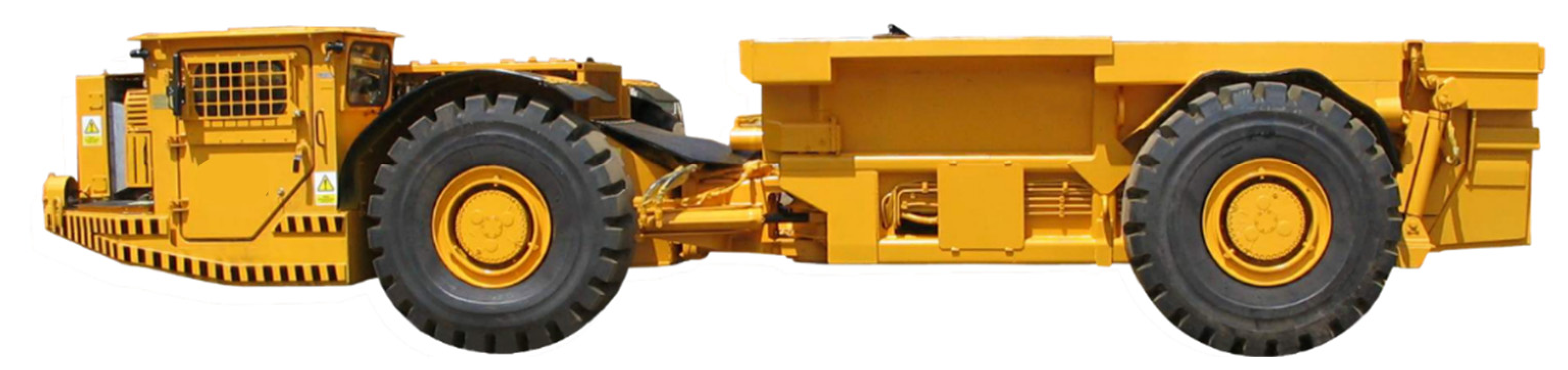
2. General Assumptions in the Machine Location Tracking Problem

This article considers an example of the cyclical operation of a haul truck (Figure 1), which consists of four basic operations:
  •  Loading the cargo box at the mining face;
  •  Hauling material to the dumping point with a grid;
  •  Unloading cargo box into a grid;
  •  Returning to the loading zone at the mining face.
A sequence comprising those four operations is called a haulage cycle, and usually, a single vehicle conducts from a few to several dozen cycles during the working shift. In practice, each individual cycle involves the passage of the machine from point A to point B along a strictly defined route. However, during one shift, there are common events where the machine changes its path. Given the Manhattan-like structure of the underground excavations (mainly straight routes, intersections at similar distances from each other, roads intersecting at 90° angles), it might seem that the problem is not that complicated and can be solved using inertial sensors commonly used in an inertial measurement unit (IMU), especially combining a three-axis accelerometer, gyroscope, and magnetometer and using the gyro integral to estimate the turn angle of the vehicle, as presented below:
α t = 0 t G y r Z x d x
where α(t) is the vehicle’s direction at moment t, and GyrZ is the gyroscope readings from the vertical axis (Z in this case). This, combined with the vehicle’s movement speed readings (which can be estimated from the accelerometer, but this solution reduces the accuracy of the results), can be easily converted into the vehicle position in the X-Y plane, as shown in [39]. This solution, however, has two related problems:
  • Gyroscope drift, being the integral of two components: a slow-changing bias instability and a higher frequency noise—angular random walk (ARW).
  • Unreliable readings from the magnetometer working in underground conditions.
These problems are related in this way: in the surface-based use cases, it is common to use magnetometer readings to correct drift by using, for example, Kalman’s or a complementary filter [40]. On the other hand, this simple solution does not use the aforementioned information on the specific excavation layout of the underground mine. That information could be used in the tracking method to reduce the drift problem, for example by identifying characteristic parts of the route and resetting the drift in those points. A concept of such a method is presented in [29], where each crossing is treated as an instance of a separate class, including its X and Y coordinates and references to the adjacent intersections. Such a graph-based construction has one significant disadvantage: when the position of the vehicle is incorrectly established once, this error affects all the subsequent readings. In the article, a simple method addressing this problem is described.
The method assumes recognizing characteristic vibration-based patterns on the vehicle route. After recognizing such a pattern, the tracking algorithm could correct the determined vehicle position burdened with an error resulting from the drift and other signal-interfering noises. The concept assumes creating a catalog of signals generated by haul trucks on small sections of routes. It would be necessary to select parts of the routes:
  •  with possibly a hardened surface, the characteristics of which are relatively constant over time, e.g., when leaving the heavy machinery chamber, or segments with a rock surface that is not quickly damaged or deformed.
  •  that would be characteristic—signals from the passage of a given section should make it possible to distinguish them from other sections of the route in an unambiguous manner and thus enable the location of a given section in space. Therefore, they cannot be, for example, flat sections of the route, on which the machine vibrations generated while driving will be practically indistinguishable.
The signals from the repeated experimental runs of the machine along such characteristic parts of the route would be used to prepare a “pattern catalog” with which the signals from the machine recorded during its regular operation should be compared. However, before such a solution could be implemented, it would be necessary to address several problems associated with it.
  • Issue 1: The different trajectory of vehicle movement within one pattern:
Driving through the same bumps at slightly different angles or bypassing them by the operator may result in significant changes in the signal recorded on the vehicle by IMU or the on-board monitoring system.
  • Solution: Create a “pattern catalog”:
Multiple passages through the same sections of the route should provide sufficiently extensive reference material that takes into account slight differences in the trajectory of the haul truck.
  • Issue 2: Different speed when covering the same sections of the route and signal length:
Different driving styles of operators and speed of covering given sections of the route may affect the overall length of the signal recorded on a given section and the distribution of characteristic signal fragments to each other.
  • Solution: DTW—Dynamic Time Warping:
DTW is an algorithm that takes into account the different lengths of the compared signals and differences in the position of their characteristic fragments.
  • Issue 3: Unexpected stoppages:
If the haul truck stops while driving along with the pattern, it may be very difficult to identify the pattern with basic methods such as cross-correlation.
  • Solution: DTW—Dynamic Time Warping:
The DTW alignment is not an injection, so it is possible to match multiple consecutive readings from one signal to one read from a signal in a catalog. As a result, many consecutive readings from the period when the machine was not moving are likely to be assigned to a short fragment of the pattern, which will minimize the alignment error.
  • Issue 4: Different machine speed and its influence on vibration level:
When the machine runs over the same sections of the route, it may result in a different level of vibrations recorded by the sensors depending on the driving speed, as described in [39,41], where linear dependence of vibrations on speed was demonstrated and classification thresholds for the adaptive vibrations to the driving speed were proposed.
  • Solution: Use of the road quality classification algorithm:
The prepared road quality classification algorithm is to some extent resistant to the variable speed of the haul truck.
  • Issue 5: Vehicle load and its influence on the vibration level:
The vehicle driving over the same route sections may result in a different level of vibrations recorded by the sensors depending on the load level of the haul truck (filling the cargo box with transported material). The conducted research shows, for example, a significantly higher level of vibrations recorded by the accelerometer in the Z-axis during the same section of the route without a load than with it.
  • Solution: Using the algorithm for identifying the road quality or limiting the method to only run with an empty or full cargo box:
The prepared road quality classification algorithm is resistant to the variable load of the machine. It is also possible to limit the application of the method to empty- or full- cargo box runs only, but this will seriously reduce the area of potential applications.
The suggested DTW algorithm as an answer to issues 2 and 3 are described in greater detail in the latter part of this article.

3. Materials and Methods

The purpose of the method is to parameterize road sections in the underground mine where the mining vehicle is moving. It comes down to the classification of signal fragments into groups corresponding to different types of road sections. The distinguishable fragments of the road will generally correspond to the type, profile, and condition of the road surface. The type and origin of the signal cause a number of the previously described phenomena, where the signal fragments corresponding to the same road segments are not identical. The main problem with this is the varying signal length. This problem is typical of the study of time series. Altogether, our efforts are related to the identification of similarity in signals (or their segments) and is commonly known in the literature as the time series matching approach. An overview of typical methods is presented in [42]. The most popular approach to measuring the similarity/dissimilarity between two time series is to estimate the Euclidean distance on the transformed representation. The method of signal similarity analysis, resistant to above the mentioned phenomenon, is Dynamic Time Warping (DTW).
The problem of detecting patterns in time series has been a current topic for a long time. This is related to the growing popularity of collecting data, a large part of which is inherently temporal data. The authors of [43] emphasized the importance of this problem, whilst also showing that DTW is a good solution. In particular, for years, scientists have been very interested in the topic of human speech recognition [44]. A signal record of each spoken word may be a pattern. These patterns can then be used to recognize words throughout a sentence. However, it is known that words are spoken at different speeds, which shows the need to use a method that is resistant to different pattern lengths. Many different ideas using DTW for this purpose can be found in the literature. For example, the authors of [45] describe the combination of this method with the Mel Frequency Cepstral Coefficient. Another idea for recognizing human speech is to use the Hidden Markov Model (HMM) [46]. In addition to human speech, a similar interesting topic is the use of DTW to recognize bird voices [47]. The obvious next step in recognizing patterns in signals is to use an appropriate classification or clustering method to automatically group similar signal segments corresponding to the same patterns. There are many examples in the literature that combine the DTW algorithm with various machine learning methods. The use of DTW with fuzzy clustering can be found in [48]. Another innovative idea is to connect DTW with neural networks [49].
In line with DTW, other methods are also commonly used, which work better or worse in specific applications. One idea is to use a measure of similarity when comparing time series. In the simplest case, the Euclidean distance is usually used for this purpose. For X , Y signals of length n , the Euclidean distance can be expressed by the following formula:
D X , Y = i = 1 n X i Y i 2 .
However, this measure has limitations in further applications. It requires both signals to be of the same length and it is not immune to time shifts. The signals are compared at the same points in time. If the patterns are of different lengths, this method will not work properly—it will not show their similarity. In this case, the so-called elastic distance measures seem to be better methods. One such method is the Longest Common Subsequence (LCSS) [50]. The method was initially developed for discrete variables. Here, the method is to find the longest string of repeating symbols [51]. It is assumed that the symbols in the sequence need not be adjacent to each other. For the extension to continuous variables, a constant threshold value is introduced, which means whether the given two values fit together. The advantage of this method is noise immunity [50]. There are also extensions to the classic string edit distance methods to time series, for example, Edit Distance for Real sequences (EDR) [52], Edit distance with Real Penalty (ERP) [53], or Time-Warp Edit Distance (TWED) [54]. These methods assume the comparison of two time series as the minimum number of transformations needed to transform one series into another. Therefore, for continuous values, it is necessary to establish a threshold that will indicate whether the two values can be considered the same or not. The disadvantages of the above methods include the need to establish a fixed threshold value. The summary of all the considered methods, along with their advantages and disadvantages, is described in Table 1.
As can be seen in the table above, the DTW algorithm is also best suited for solving the problem presented in this case. The main reason here is the fact that, among the other methods, it performs the best in the case of stretching or shortening of some fragments of the signal, which would correspond to the vehicle operator covering the given route fragments more slowly or quickly, respectively. Similarly, it is also best when a given pattern is disturbed, e.g., by a longer fragment of the signal corresponding to the machine’s stoppage.

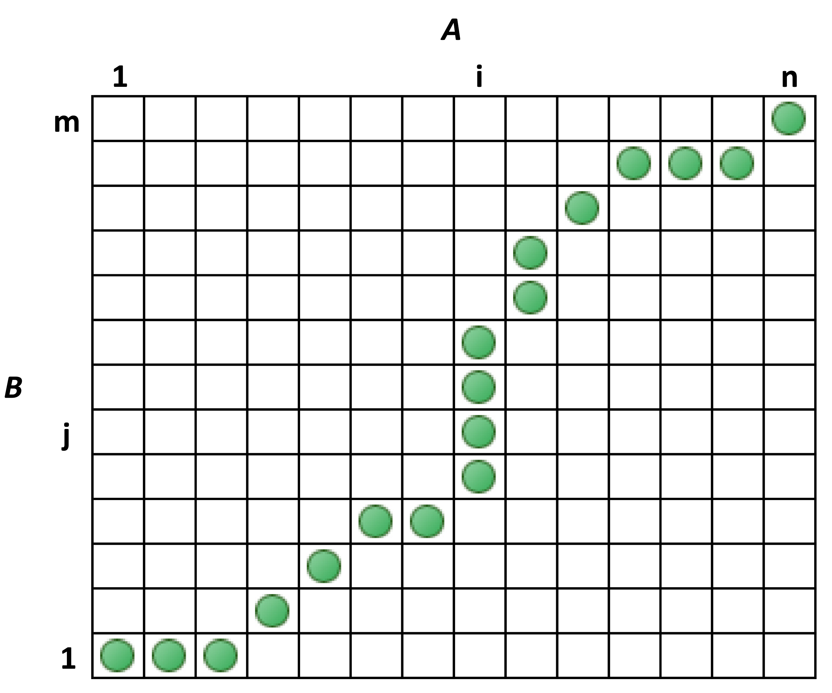
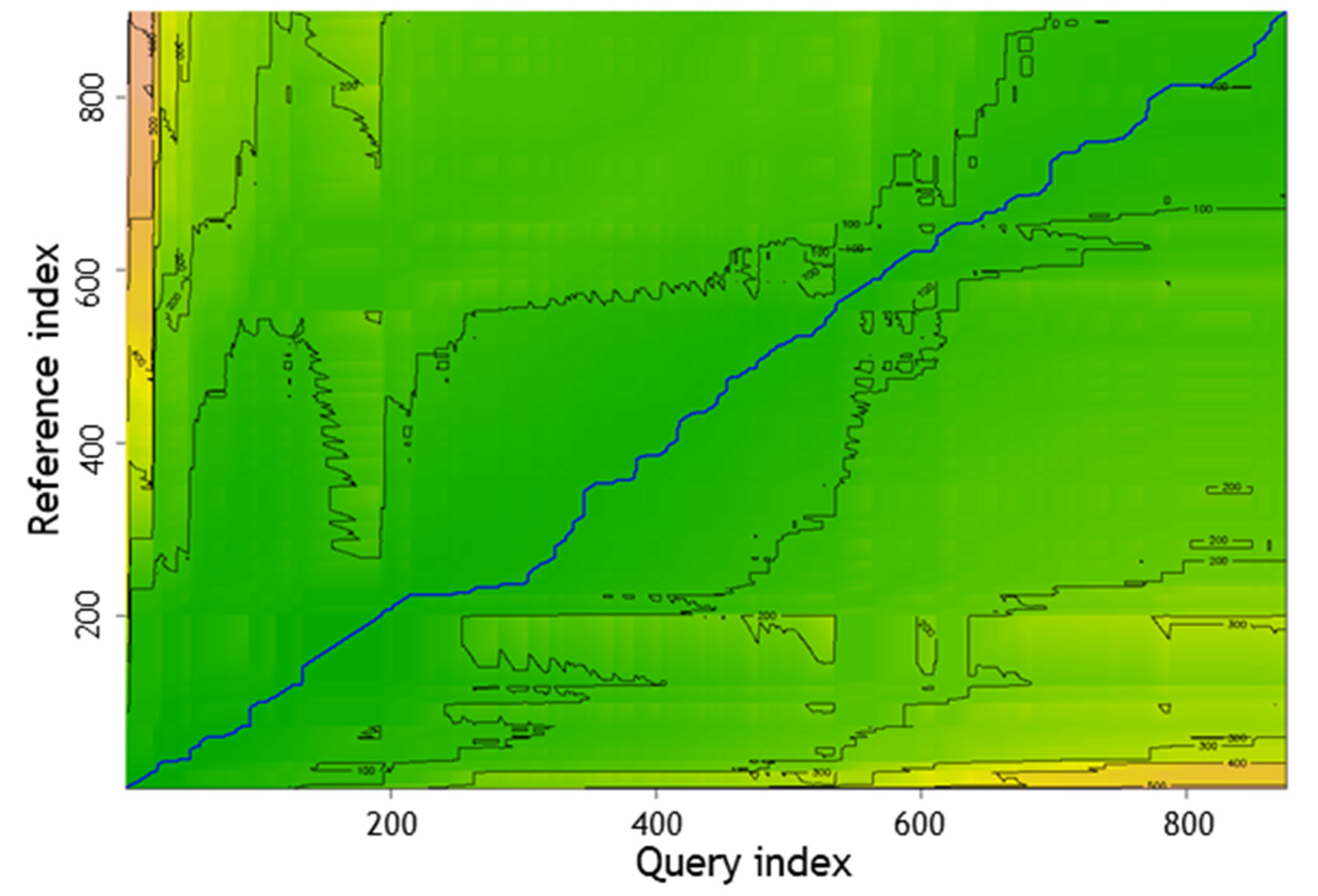
3.1. Dynamic Time Warping

As explained earlier, Dynamic Time Warping (DTW) is one of the algorithms for measuring the similarity between two signals (time series) that may differ in length. The idea of the algorithm in the form of a two-dimensional matrix is presented in Figure 2. Values in the following columns and rows correspond to two signals respectively (e.g., A and B). Let’s consider the following two time series:
A = a 1 ,   a 2 , ,   a i ,   ,   a n , B = b 1 , b 2 , ,   b j ,   ,   b m .
The presented matrix symbolizes all possible matches of the value of signal A to the value of signal B. The green points symbolize the optimal match of two signals, found by DTW. The optimal solution is chosen by minimizing the Euclidean distance between the points. The different length of the signals implies the necessity to match at least one value from the shorter signal to several values from the longer signal (surjection). This is illustrated by points arranged vertically or horizontally.
The above example shows only when the algorithm finds the optimal match indicated by the smallest Euclidean distance value. The values of this distance for each pair of readings, normalized to the range (0, 1), correspond to the probability of matching this pair, where 0 is a full match and 1 is no match. The pseudo-code of the Dynamic Time Warping algorithm is presented in Algorithm 1.
Algorithm 1. Dynamic Time Warping algorithm pseudo-code [55]
//v1 = (a1,…,an), v2 = (b1,…,bm)—time series with n and m observations respecitvely
DTW(v1, v2) {
      Let a two dimensional data matrix S be the store of similarity measures
      such that S[0,…,n, 0,…,m], and i, j, are loop index, cost is an integer.
      // data matrix initialization
      S[0, 0] := 0
      FOR i := 1 to m DO LOOP
            S[0, i] := ∞
      END
      FOR i := 1 to n DO LOOP
            S[i, 0] := ∞
      END
      // incrementally fill in the similarity matrix with the differences of the two time series
      FOR i := 1 to n DO LOOP
            FOR j := 1 to m DO LOOP
               // d function measures the distance between the two points
               cost := d(v1[i], v2[j])
               S[i, j] := cost + MIN(S[i-1, j], S[i, j−1], S[i-1, j−1])
            END
      END
      RETURN S[n, m]
}

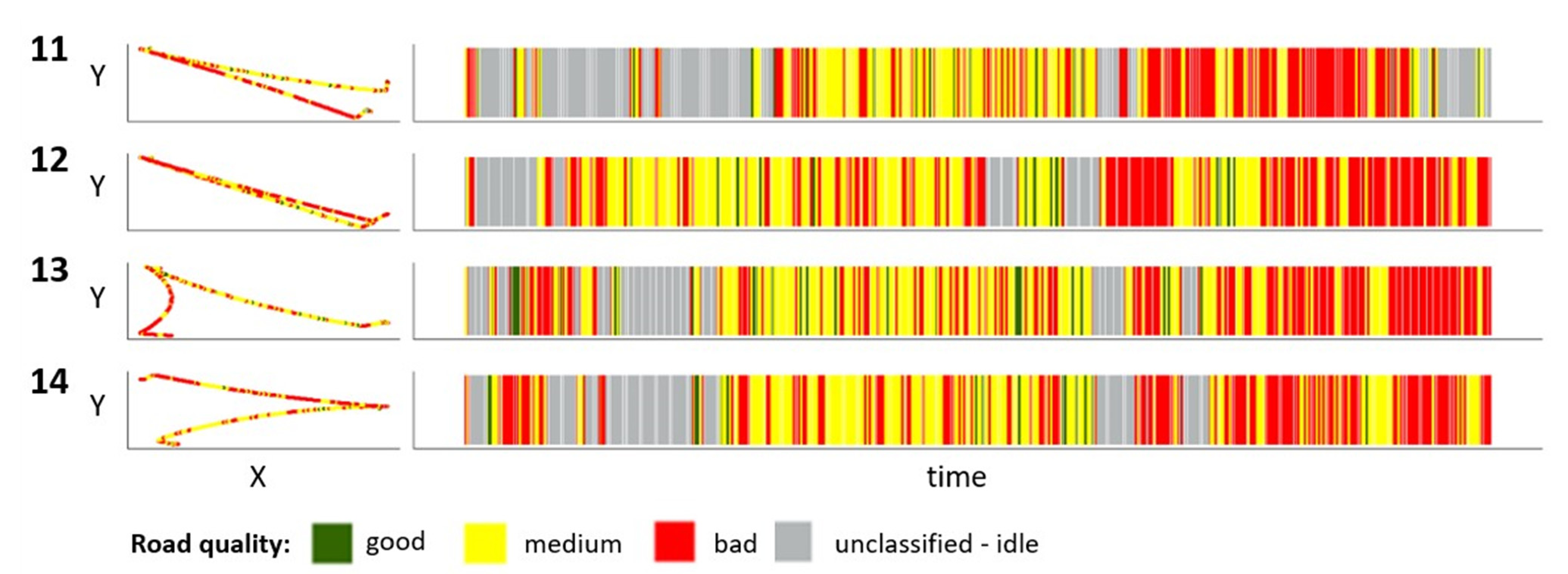
3.2. The Idea of Recognizing the Pattern of the Road

The process of recognizing fragments of the route on which the machine moves can be presented in the following steps:
  •  Creating a catalog of patterns concerning various types of road fragments.
  •  Iterative comparison of successive cut signal fragments with the directory using DTW.
  •  Recording the value of the normalized DTW distance for each of the patterns from the catalogs in the subsequent fragments of signals.
  •  Choosing the best match among the patterns in the catalog to the tested signal.
This concept is also presented in Figure 3.
The way in which the described method can be used in the process of correcting the vehicle location is shown in Figure 4.

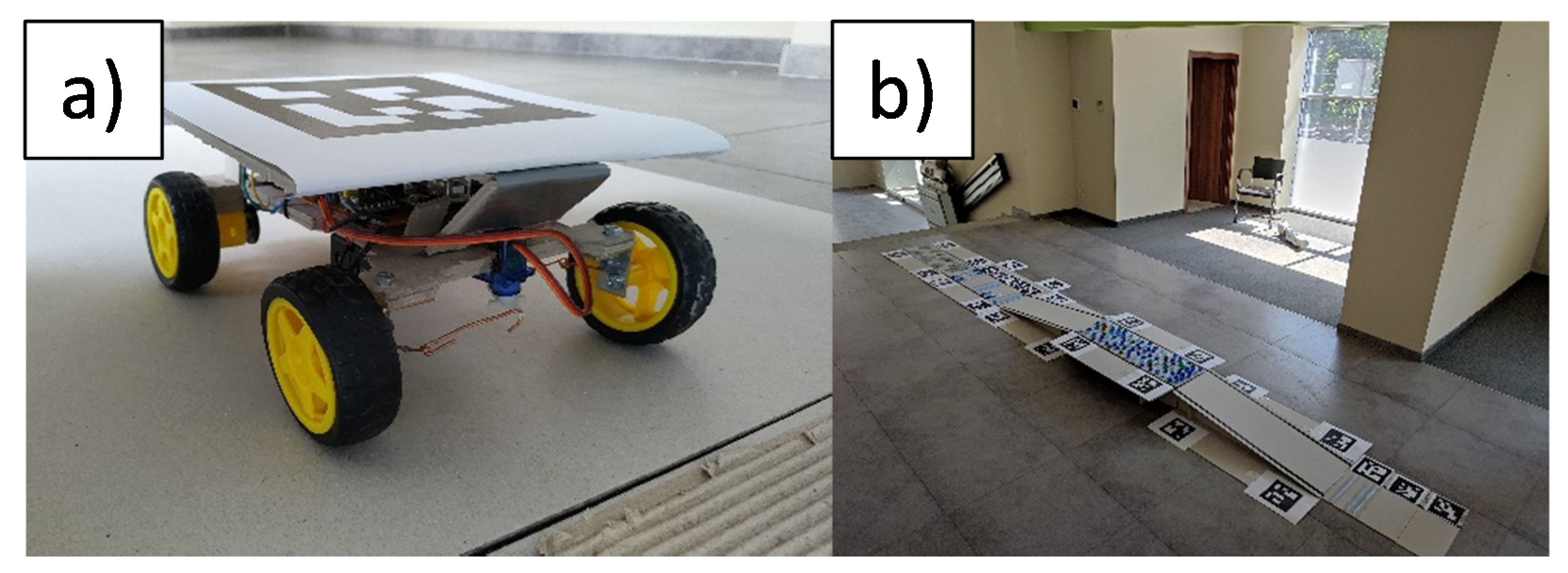
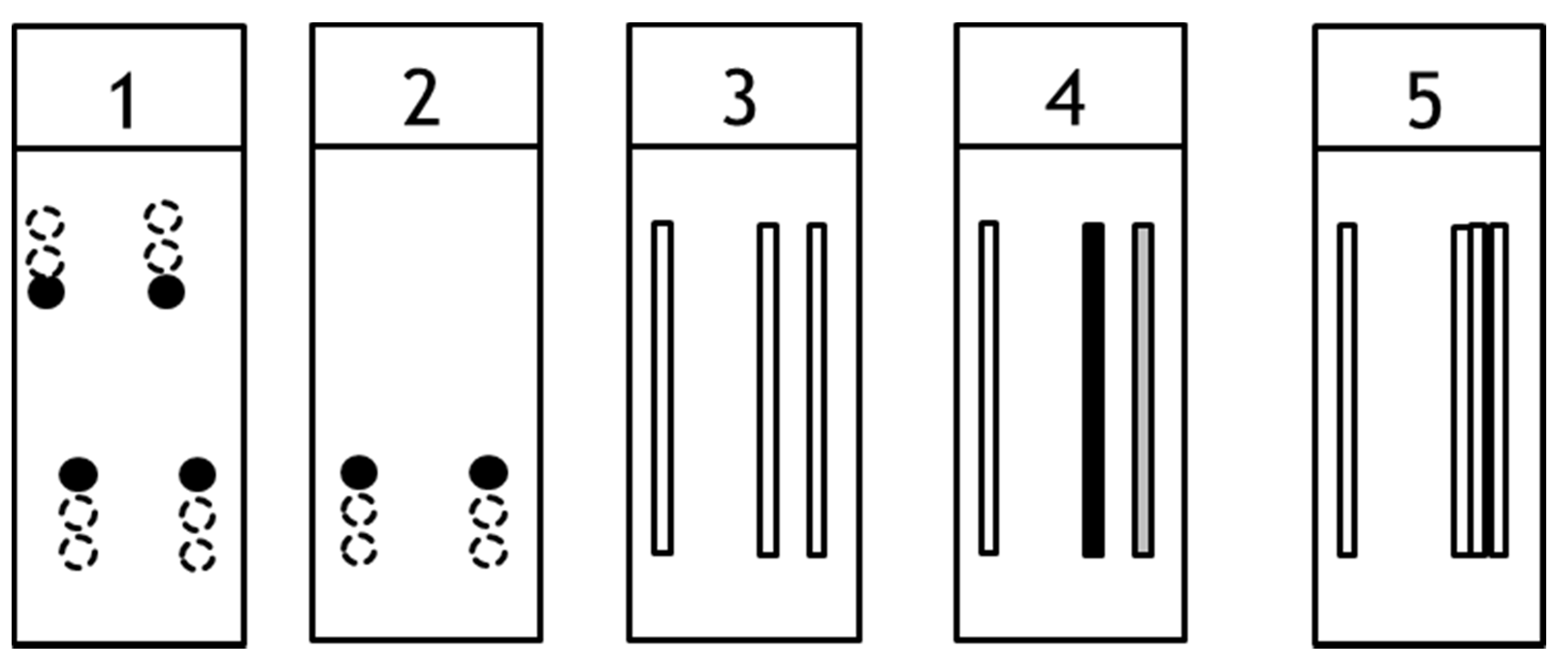
3.3. Description of the Experiment in Laboratory Conditions

In the first step, the proposed algorithm was tested on a test rig with the use of a wheeled robot (Figure 5a) with sensors enabling, among other things, the measurement of driving speed, vibration, gyroscope, and accelerometer signals.
As a part of the experiments, five different 18 cm wide road modules (panels) made of cardboard, bottle caps, and pens were prepared. The combinations of these modules created characteristic patterns on the longer route. The scheme of the prepared patterns is presented in Figure 6. The scheme shows the following patterns: (1) alternating caps; (2) caps evenly distributed on one side; (3) three consecutive humps at different distances, with the same height; (4) modification of pattern three with different hump heights; (5) two humps of the same height, but the second is three times as long.
During the experiment, 10 training drives were performed to learn every single pattern, and then three test drives (for each module) were conducted to verify the pattern recognition algorithm. The training drives were made using the following panel combinations:
(a)
 panels 1–5 arranged directly one after the other,
(b)
 panels 1, 3, and 5 arranged directly one after the other,
(c)
 isolated panels 1, 3, and 5.
The test routes were created by placing one of the patterns at the beginning and the other panels later. Such drives were made for each of the a–c patterns.

3.4. Application of the Algorithm

The signal used for pattern recognition is the Z-axis accelerometer values. These are the linear acceleration values measured along the axis perpendicular to the plane on which the vehicle is driving. These values are therefore proportional to the vibration on this axis and seem to correspond best to the problem presented. Figure 7 shows four examples of accelerometer signals measured during training drives for the first pattern—(a) panels 1–5 directly one after the other. It can be seen that the signals vary in length and it is difficult to visually determine the similarities between them.
Figure 8 shows the graphs of the Z-axis accelerometer for three test drives along the route containing pattern (a). It can be seen that there is a greater variance in the first part of the signal, which corresponds to driving through the panels of the pattern that were placed at the start of the route. At the same time, it can be seen that this fragment is much longer, containing the first 7–8 s of the signal (training drives lasted up to 2 s). This is mainly due to the necessity of frequent correction of the vehicle’s route and deliberate stopping before entering the ramp that was placed behind the pattern.
The accelerometer measurements during the test drives were compared with the signals corresponding to the pattern for each training drive. An example of the results of the normalized Euclidean distance, which is the result of the DTW algorithm, is presented in Figure 9. It can be seen that the signals look very similar in each drive, which results from experimenting in laboratory conditions. It is not expected to obtain similar repeatability during subsequent drives in industrial conditions. In each case, the moment of the pattern occurrence was correctly detected as the fragment with the lowest normalized DTW distance. In Figure 9, these are the fragments marked with a green circle.
The same method was repeated for the subsequent shorter patterns—(b) composed of panels 1, 3, and 5 arranged directly one after the other; and (c) isolated panels 1, 3, and 5. In case (b), despite the shortened pattern, good results were still obtained, where the detection of the moment of pattern occurrence was possible for each signal (an example of matches is presented in Figure 10). However, there were signals in which too high a threshold resulted in a wrong match (the fragment marked with a yellow circle).
On the other hand, when using only single panels as a pattern, it cannot be said that the DTW method allows the determination of the moment of pattern occurrence. Figure 11 shows exemplary results using panel number 3. The erroneous detection of the moment of pattern occurrence is marked in red, and the fragment that should have been detected is marked in green. However, it should be remembered that in this case, the length of the pattern was about 18 cm, which is approximately the wheelbase of the remote vehicle used for testing. This shows that the pattern must be long and complex enough to be detected by the DTW algorithm.
The summary of the tests conducted in the laboratory stands for different lengths of the pattern are presented in Table 2. As it can be seen, the proposed method returns reliable results for the patterns consisting of five and three panels (90 cm and 54 cm respectively), but a one panel pattern turned out to be insufficient for the problem being considered.

4. Application to Industrial Data

Using data from vehicles operating in industrial conditions, it was decided to conduct a simple simulation to verify the conclusions obtained during laboratory tests. The machines have a built-in on-board monitoring system that measures different types of operational parameters, such as vehicle speed. Additionally, the machine was equipped with an IMU, which allows the obtainment of a signal from an accelerometer. The speed and Z-axis accelerometer (direction: up-down) signals made it possible to create a three-state classification of road quality [39,41]. The results of this classification will be used as a signal to test the possibility of recognizing road patterns. Sample results for selected cycles of haulage process from one shift are presented in Figure 11. Subsequent cycles are performed on the same routes. Additionally, in each cycle, the machine traveled to a set point and returned along the same route. However, separate patterns were created for both of these drives. Similarities between the signals can be seen; however, there are different lengths of the same patterns, and time shifts between different sections are also visible.
When comparing two of the presented paths by using DTW implementation in the DTW library in R language, a cumulative cost density with an over-imposed warping path can be plotted using the dtwPlotDensity function. This, applied to cycles 13 and 14 from Figure 12, is presented in Figure 13.
The blue line represents an optimal alignment on a field, where the high cost of an assignment has been presented with a red-orange color and low cost with a green color.

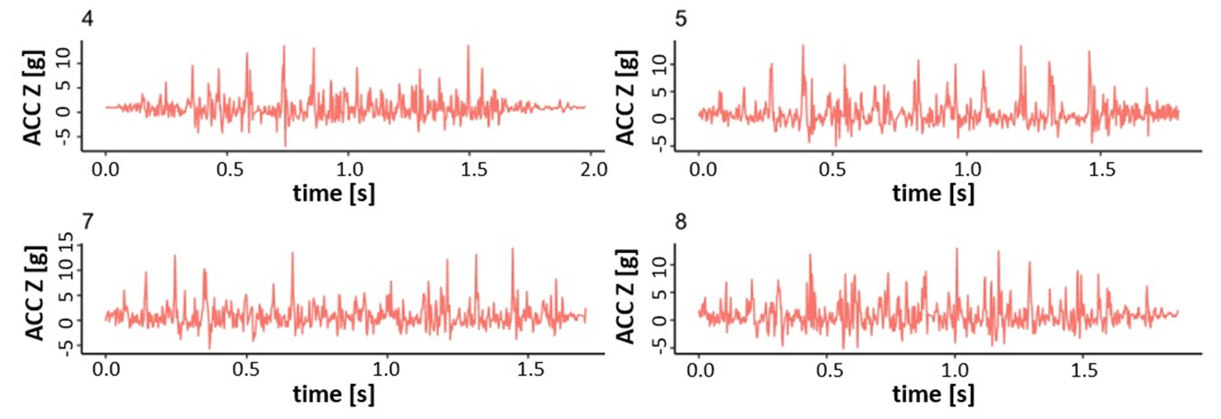
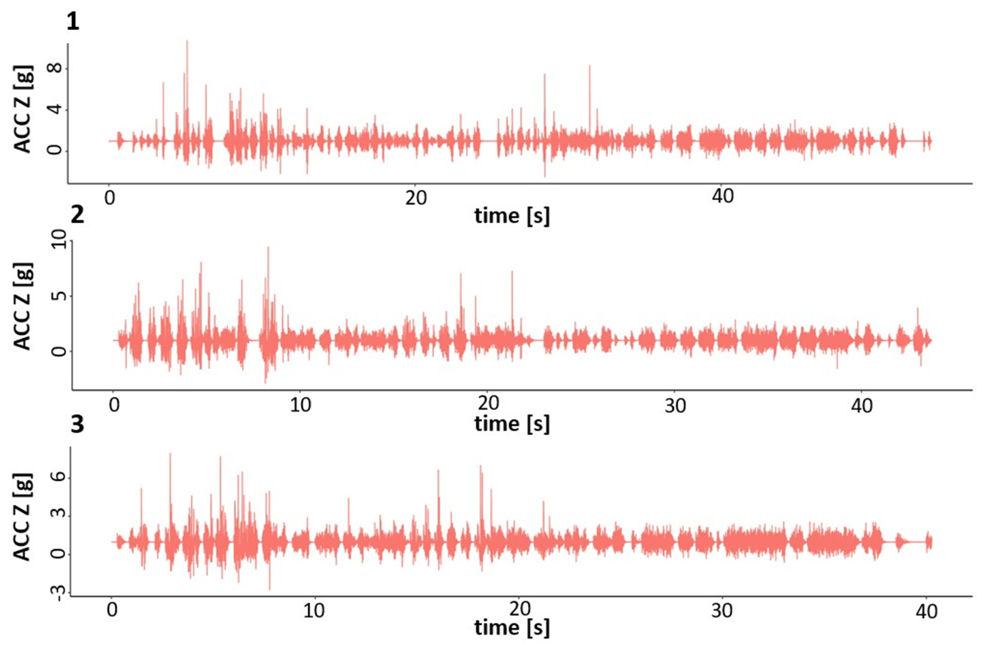
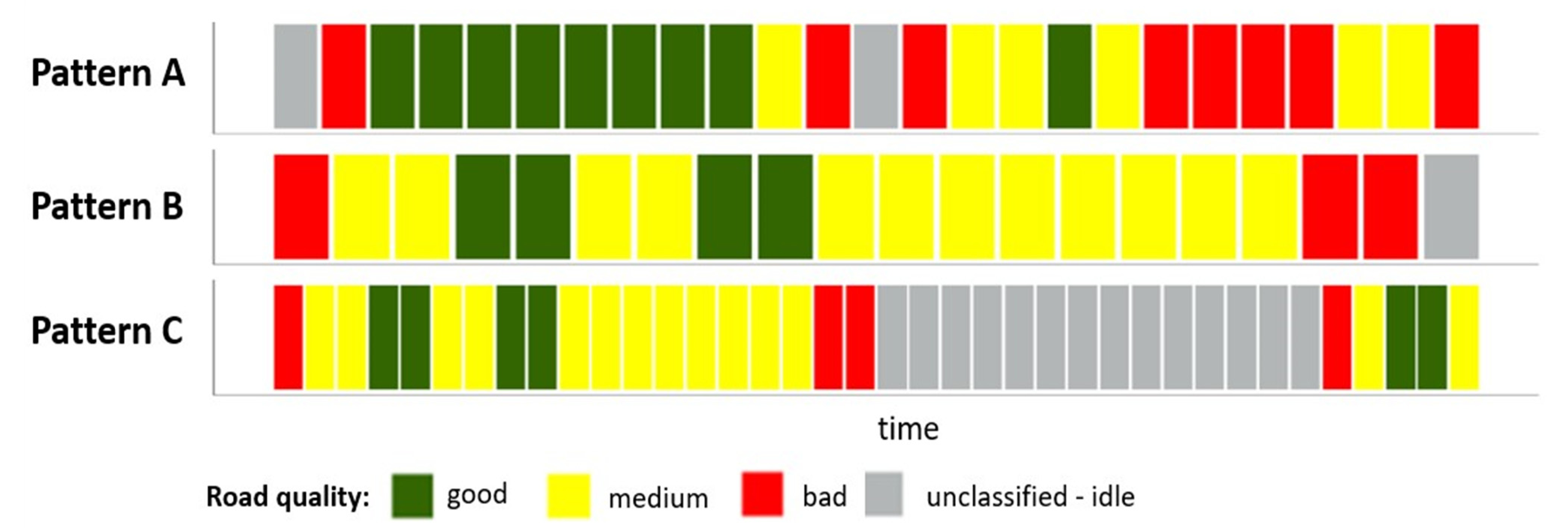
4.1. Creating Patterns

In the signals, it was decided to select fragments that would constitute patterns. For example, for cycle number 13, three patterns were selected: A (duration 24 s), B (19 s) C (37 s), which are shown in Figure 14.
Then, to expand the training sample, it was decided to simulate the distortion of the patterns. This was done by lengthening or shortening some fragments several times. An example of a modification record for a signal consisting of 19 readings can be presented as follows:
a r t i f i c i a l _ s e r i e s = 1 ,   1 ,   1 ,   1 ,   3 ,   1 ,   1 ,   1 ,   1 ,   1 ,   1 ,   1 ,   5 ,   1 ,   1 ,   1 ,   1 ,   1 ,   1 .
Successive values correspond to the number of repetitions of each subsequent signal fragment. This means that the output signal will now be 25 readings long, the first four readings will not be changed, the fifth one will be repeated three times, etc.

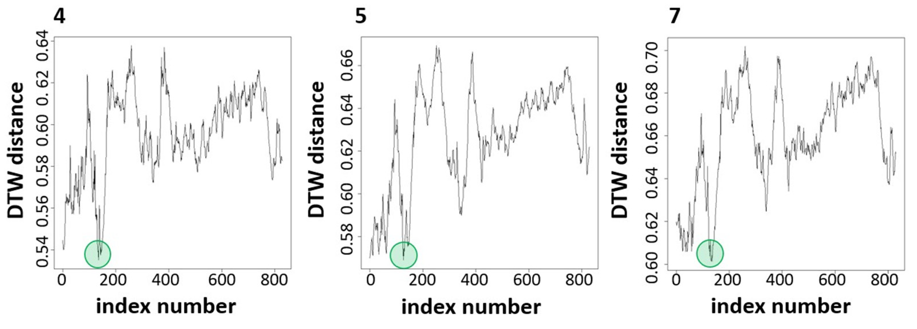
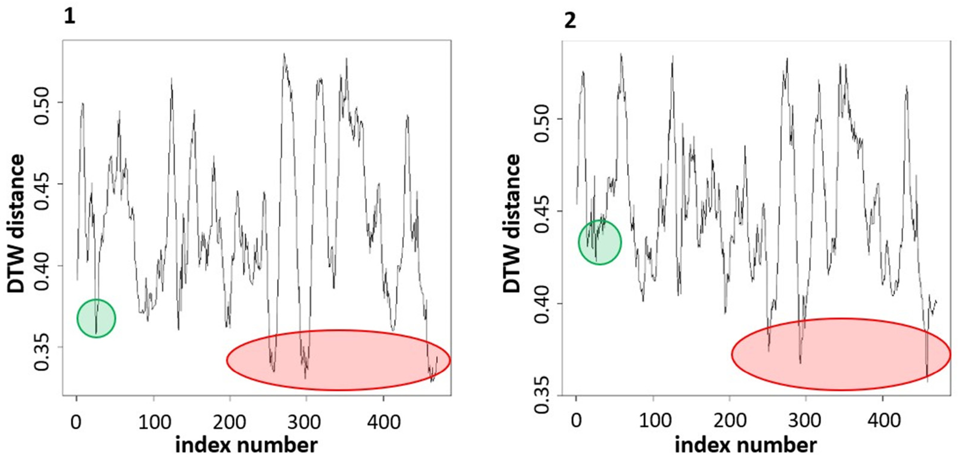
4.2. Pattern Detection

The patterns determined in this way and their distortions could be found in raw signals using the DTW algorithm. An exemplary adjustment of the B pattern and its two modifications to the signal using the DTW method is shown in Figure 15. It can be seen that the DTW distance signal for distorted patterns changes slightly, but the detection of the moment of pattern occurrence is still possible (the fragment is marked on the signal with an ellipse). This shows that the discussed method also allows the detection of path patterns when applied to industrial data. Additionally, it is resistant to different signal lengths, which is a key problem in the case of time series. However, this method would require more comprehensive tests of real conditions, strictly in order to confirm its effectiveness.

5. Conclusions

The location of LHD in underground mining excavations is a key issue not only from the point of view of navigation and automation of the haulage process and increasing safety through anti-collision systems, but also the development of advanced analytics in the field of predictive traffic maintenance, production planning, and optimization of horizontal transport. For indoor conditions, especially underground, the range of available technology is limited. Internal sensors such as inertial, odometry, and heading angle are commonly used to estimate the absolute position of the vehicle in the fixed real-world coordinate system. Their main disadvantage is high susceptibility to scale errors and offsets which lead to unbounded errors on the position estimate. For this reason, it is necessary to correct them through additional sources of information from the LHD environment. In practice, solutions based on the detection of artificial beacons or natural features of the environment are used. Therefore, such solutions require the fusion of data from internal sensors embedded on the machine and the expansion of the infrastructure in its surroundings, which is not cost-effective both from the point of view of construction and maintenance of such a system. For the needs of post-factum analytics development, the mining industry is expected to develop a cheap and possibly non-invasive system, preferably based on a single data source. For this reason, we fill this niche by proposing an approach based solely on the accelerometer signal and digital map. In the article, we have focused on the issue of identifying the characteristic road surface patterns that will serve as control points for the correction of the estimated movement path on the map. In our case, the task comes down to recognizing the patterns hidden in the accelerometer signal along the Z-axis resulting from different height profiles of pavement. These patterns are not visible in the raw signals; therefore, we have proposed using the three-state road quality classification procedure for their extraction. Having a pattern database for various local mine points, we can further identify them while processing subsequent signals. This issue is related to the identification of similarity in signals (or their segments) and is commonly known in the literature as the time series matching approach. The most popular approach to measuring the similarity/dissimilarity between two time series is to estimate the Euclidean distance on the transformed representation. In our case, we chose the DTW algorithm because it is resistant to the boundary conditions of the investigated task (different runs of the machine in relation to the width of the road, unplanned stoppages, and different driving speeds resulting in different signal lengths and pattern distribution, the influence of driving speed and cargo box load on vibration level, and input data in flag form). The described concept was presented and validated on a laboratory stand, with the real industrial data being recorded by the LHD vehicle operating in an underground mine. The minimal length of the pattern was established as three times the wheelbase of the vehicle. For that pattern length, we were able to accurately identify different patterns for each of the three conducted test drives. The advantage of using the DTW method is the algorithm robustness to the signal distortion, consisting of the stretching or shortening of its specific fragments, which would correspond to operators covering given parts of the route more slowly or quickly, respectively.

Author Contributions

Conceptualization, P.S. and B.J.; methodology, P.S. and B.J.; validation, A.S. and W.K.; formal analysis, P.S.; investigation, P.S., B.J., and A.S.; resources, P.S., B.J., and A.S.; data curation, A.S.; writing—original draft preparation, P.S., B.J., and W.K.; writing—review and editing, P.S., B.J., W.K., and A.S.; visualization, B.J. and W.K.; supervision, P.S.; project administration, P.S. All authors have read and agreed to the published version of the manuscript.

Funding

This research was partially funded by the European Union’s Horizon 2020 research and innovation programme under grant agreement No. 780883.

Institutional Review Board Statement

Not applicable.

Informed Consent Statement

Not applicable.

Data Availability Statement

Not applicable.

Conflicts of Interest

The authors declare no conflict of interest.

References

  1. Brzychczy, E.; Gackowiec, P.; Liebetrau, M. Data Analytic Approaches for Mining Process Improvement—Machinery Utilization Use Case. Resources 2020, 9, 17. [Google Scholar] [CrossRef] [Green Version]
  2. Wojaczek, A.; Wojaczek, A. Monitoring the environment and machines in underground mine. Zesz. Nauk. Inst. Gospod. Surowcami Miner. Pol. Akad. Nauk. 2017, 99, 57–70. [Google Scholar]
  3. Stefaniak, P.K.; Zimroz, R.; Sliwinski, P.; Andrzejewski, M.; Wyłomanska, A. Multidimensional signal analysis for technical condition, operation and performance understanding of heavy duty mining machines. In Proceedings of the International Conference on Condition Monitoring of Machinery in Non-Stationary Operation, Lyon, France, 15–17 December 2014; Springer: Cham, Switzerland; Berlin/Heidelberg, Germany, 2014; pp. 197–210. [Google Scholar]
  4. Gustafson, A.; Paraszczak, J.; Tuleau, J.; Schunnesson, H. Impact of technical and operational factors on effectiveness of automatic load-haul-dump machines. Min. Technol. 2017, 126, 185–190. [Google Scholar]
  5. Wodecki, J.; Stefaniak, P.; Michalak, A.; Wyłomańska, A.; Zimroz, R. Technical condition change detection using Anderson–Darling statistic approach for LHD machines–engine overheating problem. Int. J. Min. Reclam. Environ. 2018, 32, 392–400. [Google Scholar] [CrossRef]
  6. Paraszczak, J.; Gustafson, A.; Schunnesson, H. Technical and operational aspects of autonomous LHD application in metal mines. Int. J. Min. Reclam. Environ. 2015, 29, 391–403. [Google Scholar]
  7. Kawalec, P. How Will the 4th Industrial Revolution Influences the Extraction Industry? Inżynieria Miner. 2019, 21, 327–334. [Google Scholar]
  8. Whittaker, W. Utilization of position and orientation data for preplanning and real time autonomous vehicle navigation. In Proceedings of the IEEE/ION PLANS, San Diego, CA, USA, 25–27 April 2006; pp. 372–377. [Google Scholar]
  9. Roberts, J.M.; Duff, E.S.; Corke, P.I. Reactive navigation and opportunistic localization for autonomous underground mining vehicles. Inf. Sci. 2002, 145, 127–146. [Google Scholar] [CrossRef]
  10. Hemami, A. A conceptual approach to automation of LHD-loaders. In Proceedings of the 5th Canadian Symposium on Mining Automation, Vancouver, BC, Canada, 27–29 September 1992; pp. 178–183. [Google Scholar]
  11. Hemami, A. Motion trajectory study in the scooping operation of an LHD-loader. IEEE Trans. Ind. Appl. 1994, 30, 1333–1338. [Google Scholar] [CrossRef]
  12. Labonte, F.; Cohen, P. Perceptual aspects of mining equipment teleoperation. In Proceedings of the 6th Canadian Symposium on Mining Automation, Montreal, QC, Canada, 16–19 October 1994. [Google Scholar]
  13. Labonte, F.; Giraud, J.; Polotski, V. Telerobotics issues in the operation of a LHD vehicle. In Proceedings of the Third Canadian Conference on Computer Applications in the Mineral Industry, Montreal, QC, Canada, 22–25 October 1995; pp. 672–681. [Google Scholar]
  14. Baiden, G. Multiple LHD teleoperation and guidance at Inco Limited. In Proceedings of the International Mining Conference; 1993. [Google Scholar]
  15. Hurteau, R.; St-Amant, M.; Laperrière, Y.; Chevrette, G. Optical guidance system for underground mine vehicles. In Proceedings of the 1992 IEEE International Conference on Robotics and Automation, Nice, France, 12–14 May 1992; IEEE Computer Society: Washington, DC, USA, 1992; pp. 639–640. [Google Scholar]
  16. Amdahl, K.; Lundström, M. Automatic Truck Saves Money Underground; World Mining: London, UK, 1972; pp. 40–44. [Google Scholar]
  17. Steele, J.P.H.; Ganesh, C.; Kleve, A. Control and scale model simulation of sensor-guided LHD mining machines. IEEE Trans. Ind. Appl. 1993, 29, 1232–1238. [Google Scholar] [CrossRef]
  18. Mäkelä, H.; Lehtinen, H.; Rintanen, K.; Koskinen, K. Navigation System for LHD machines. In Intelligent Autonomous Vehicles 1995; Pergamon Press: Oxford, UK, 1995; pp. 295–300. [Google Scholar]
  19. Scheding, S.; Dissanayake, G.; Nebot, E.M.; Durrant-Whyte, H. An experiment in autonomous navigation of an underground mining vehicle. IEEE Trans. Robot. Autom. 1999, 15, 85–95. [Google Scholar] [CrossRef] [Green Version]
  20. Eriksson, G. Automatic loading and dumping using vehicle guidance in a Swedish mine. In Proceedings of the 1st International Symposium on Mine Mechanization and Automation, Golden, CO, USA, 10–13 June 1991; Volume 2, pp. 15–33. [Google Scholar]
  21. Ishimoto, H.; Tsubouchi, T.; Sarata, S. A practical trajectory following of an articulated steering type vehicle. In Field and Service Robotics; Springer: London, UK, 1998; pp. 397–404. [Google Scholar]
  22. Hemami, A.; Polotski, V. Path tracking control problem formulation of an LHD loader. Int. J. Robot. Res. 1998, 17, 193–199. [Google Scholar] [CrossRef]
  23. Thrun, S.; Burgard, W.; Fox, D. A real-time algorithm for mobile robot mapping with applications to multi-robot and 3D mapping. In Proceedings of the 2000 ICRA, Millennium Conference, IEEE International Conference on Robotics and Automation, Symposia Proceedings (Cat. No. 00CH37065), San Francisco, CA, USA, 24–28 April 2000; IEEE: Piscataway, NJ, USA, 2000; Volume 1, pp. 321–328. [Google Scholar]
  24. Duff, E.S.; Roberts, J.M.; Corke, P.I. Automation of an underground mining vehicle using reactive navigation and opportunistic localization. In Proceedings of the 2003 IEEE/RSJ International Conference on Intelligent Robots and Systems (IROS 2003) (Cat. No. 03CH37453), Las Vegas, NV, USA, 27–31 October 2003; IEEE: Piscataway, NJ, USA, 2003; Volume 4, pp. 3775–3780. [Google Scholar]
  25. Larsson, J.; Broxvall, M.; Saffiotti, A. Laser based intersection detection for reactive navigation in an underground mine. In Proceedings of the 2008 IEEE/RSJ International Conference on Intelligent Robots and Systems, Nice, France, 22–26 September 2008; IEEE: Piscataway, NJ, USA, 2008; pp. 2222–2227. [Google Scholar]
  26. Mäkelä, H. Overview of LHD navigation without artificial beacons. Robot. Auton. Syst. 2001, 36, 21–35. [Google Scholar] [CrossRef]
  27. Bakambu, J.N.; Polotski, V. Autonomous system for navigation and surveying in underground mines. J. Field Robot. 2007, 24, 829–847. [Google Scholar] [CrossRef]
  28. Yulong, Q.; Qingyong, M.; Xu, T. Research on Navigation Path Planning for an Underground Load Haul Dump. J. Eng. Sci. Technol. Rev. 2015, 8, 102–109. [Google Scholar] [CrossRef]
  29. Skoczylas, A.; Stefaniak, P. Localization System for Wheeled Vehicles Operating in Underground Mine Based on Inertial Data and Spatial Intersection Points of Mining Excavations. In Intelligent Information and Database Systems, Proceedings of the 13th Asian Conference, ACIIDS 2021, Phuket, Thailand, 7–10 April 2021; Springer: Berlin/Heidelberg, Germany, 2021; pp. 824–834. [Google Scholar]
  30. Witulska, J.; Stefaniak, P.; Jachnik, B.; Skoczylas, A.; Śliwiński, P.; Dudzik, M. Recognition of LHD Position and Maneuvers in Underground Mining Excavations—Identification and Parametrization of Turns. Appl. Sci. 2021, 11, 6075. [Google Scholar] [CrossRef]
  31. Walas, K.; Kanoulas, D.; Kryczka, P. Terrain classification and locomotion parameters adaptation for humanoid robots using force/torque sensing. In Proceedings of the 2016 IEEE-RAS 16th International Conference on Humanoid Robots (Humanoids), Cancun, Mexico, 15–17 November 2016; IEEE: Piscataway, NJ, USA, 2016; pp. 133–140. [Google Scholar]
  32. Mrva, J.; Faigl, J. Feature Extraction for Terrain Classification with Crawling Robots. In ITAT; Charles University: Prague, Czech Republic, 2015; pp. 179–185. [Google Scholar]
  33. Dallaire, P.; Walas, K.; Giguere, P.; Chaib-draa, B. Learning terrain types with the pitman-yor process mixtures of gaussians for a legged robot. In Proceedings of the 2015 IEEE/RSJ International Conference on Intelligent Robots and Systems (IROS), Hamburg, Germany, 28 September–3 October 2015; IEEE: Piscataway, NJ, USA, 2015; pp. 3457–3463. [Google Scholar]
  34. Filitchkin, P.; Byl, K. Feature-based terrain classification for littledog. In Proceedings of the 2012 IEEE/RSJ International Conference on Intelligent Robots and Systems, Vilamoura-Algarve, Portugal, 7–12 October 2012; IEEE: Piscataway, NJ, USA, 2012; pp. 1387–1392. [Google Scholar]
  35. Walas, K. Terrain classification and negotiation with a walking robot. J. Intell. Robot. Syst. 2015, 78, 401–423. [Google Scholar] [CrossRef] [Green Version]
  36. Skoczylas, A.; Stachowiak, M.; Stefaniak, P.; Jachnik, B. Terrain Classification Using Neural Network Based on Inertial Sensors for Wheeled Robot. In Recent Challenges in Intelligent Information and Database Systems; Springer: Berlin/Heidelberg, Germany, 2021. [Google Scholar] [CrossRef]
  37. Gustafson, A. Automation of Load Haul Dump Machines; Luleå Tekniska Universitet: Luleå, Sweden, 2011. [Google Scholar]
  38. KGHM ZANAM. Available online: https://www.kghmzanam.com/en/produkty/mining-machinery/haul-trucks/haul-truck-cb4p-24k/ (accessed on 21 July 2021).
  39. Stefaniak, P.; Anufriiev, S.; Skoczlas, A.; Bartosz, J.; Sliwinski, P. Method to haulage path estimation and road-quality assessment using inertial sensors on LHD machines. Vietnam. J. Comput. Sci. 2020. [Google Scholar] [CrossRef]
  40. Deibe, Á.; Antón Nacimiento, J.A.; Cardenal, J.; López Peña, F. A Kalman Filter for Nonlinear Attitude Estimation Using Time Variable Matrices and Quaternions. Sensors 2020, 20, 6731. [Google Scholar] [CrossRef]
  41. Skoczylas, A.; Stefaniak, P.; Anufriiev, S.; Jachnik, B. Road Quality Classification Adaptive to Vehicle Speed Based on Driving Data from Heavy Duty Mining Vehicles. In Proceedings of the International Conference on Intelligent Computing & Optimization, Hua Hin, Thailand, 22–23 April 2021; Springer: Cham, Germany, 2020; pp. 777–787. [Google Scholar]
  42. Fu, T.C. A review on time series data mining. Eng. Appl. Artif. Intell. 2011, 24, 164–181. [Google Scholar] [CrossRef]
  43. Berndt, D.J.; Clifford, J. Using dynamic time warping to find patterns in time series. In Proceedings of the KDD Workshop, Seattle, WA, USA, 31 July–1 August 1994; Volume 10, pp. 359–370. [Google Scholar]
  44. Vintsyuk, T.K. Speech discrimination by dynamic programming. Cybernetics 1968, 4, 52–57. [Google Scholar] [CrossRef]
  45. Muda, L.; Begam, M.; Elamvazuthi, I. Voice recognition algorithms using mel frequency cepstral coefficient (MFCC) and dynamic time warping (DTW) techniques. arXiv 2010, arXiv:1003.4083. [Google Scholar]
  46. Prasad, V. Voice recognition system: Speech-to-text. J. Appl. Fundam. Sci. 2015, 1, 191. [Google Scholar]
  47. Jančovič, P.; Köküer, M.; Zakeri, M.; Russell, M. Unsupervised discovery of acoustic patterns in bird vocalisations employing DTW and clustering. In Proceedings of the 21st European Signal Processing Conference (EUSIPCO 2013), Marrakech, Morocco, 9–13 September 2013; IEEE: Piscataway, NJ, USA, 2013; pp. 1–5. [Google Scholar]
  48. Chen, G.; Wei, Q.; Zhang, H. Discovering similar time-series patterns with fuzzy clustering and DTW methods. In Proceedings of the Joint 9th IFSA World Congress and 20th NAFIPS International Conference (Cat. No. 01TH8569), Vancouver, BC, Canada, 25–28 July 2001; IEEE: Piscataway, NJ, USA, 2001; Volume 4, pp. 2160–2164. [Google Scholar]
  49. Iwana, B.K.; Frinken, V.; Uchida, S. DTW-NN: A novel neural network for time series recognition using dynamic alignment between inputs and weights. Knowl. Based Syst. 2020, 188, 104971. [Google Scholar] [CrossRef]
  50. Vlachos, M.; Kollios, G.; Gunopulos, D. Discovering similar multidimensional trajectories. In Proceedings of the 18th International Conference on Data Engineering, San Jose, CA, USA, 26 February–1 March 2002; IEEE: Piscataway, NJ, USA, 2002; pp. 673–684. [Google Scholar]
  51. Hirschberg, D.S. Algorithms for the longest common subsequence problem. J. ACM JACM 1977, 24, 664–675. [Google Scholar] [CrossRef] [Green Version]
  52. Chen, L.; Özsu, M.T.; Oria, V. Robust and fast similarity search for moving object trajectories. In Proceedings of the 2005 ACM SIGMOD International Conference on Management of Data, Baltimore, MD, USA, 14–16 June 2005; pp. 491–502. [Google Scholar]
  53. Chen, L.; Ng, R. On the marriage of lp-norms and edit distance. In Proceedings of the Thirtieth International Conference on Very Large Data Bases, Toronto, ON, Canada, 31 August–3 September 2004; Volume 30, pp. 792–803. [Google Scholar]
  54. Marteau, P.F. Time warp edit distance with stiffness adjustment for time series matching. IEEE Trans. Pattern Anal. Mach. Intell. 2008, 31, 306–318. [Google Scholar] [CrossRef] [Green Version]
  55. Fong, S. Using hierarchical time series clustering algorithm and wavelet classifier for biometric voice classification. J. Biomed. Biotechnol. 2012, 2012, 215019. [Google Scholar] [CrossRef] [Green Version]
Figure 1. Investigated object—underground haul truck used in the conducted experiments. Load capacity: 24,000 kg, engine power: 172 kW, top speed: 25 km/h [38].
Applsci 11 06751 g001
Figure 2. The matchings for the compared A and B signals can be presented on a two-dimensional matrix.
Applsci 11 06751 g002
Figure 3. Concept of road pattern recognition from accelerometer readings.
Applsci 11 06751 g003
Figure 4. The concept of using the presented method in the problem of tracking mining vehicles in underground excavation: (a) vehicle position as calculated using method described in [39]; (b) selection of characteristic road patterns; (c) vehicle position after correction, using methods described in [29]; (d) recognition of patterns using DTW algorithm for further evaluation and path correction. It can be seen that during one haulage cycle, the same part of the route is covered by the vehicle in two different directions; therefore, two patterns should be saved in the catalog.
Applsci 11 06751 g004
Figure 5. Test rig used in experiments: (a) wheeled robot, (b) exemplary layout of modular mock-up simulating road conditions in an underground mine.
Applsci 11 06751 g005
Figure 6. Schemes of patterns prepared for the experiments.
Applsci 11 06751 g006
Figure 7. Examples of accelerometer signals for training driving for pattern (a), composed of panels 1–5.
Applsci 11 06751 g007
Figure 8. Accelerometer signals for three test drives for the pattern (a) composed of panels 1–5.
Applsci 11 06751 g008
Figure 9. Normalized DTW distance between signals for three test drives and training drives for pattern (a), composed of panels 1–5.
Applsci 11 06751 g009
Figure 10. DTW distance for selected training and test drives for pattern (b), composed of panels 1, 3, and 5 arranged directly one after the other.
Applsci 11 06751 g010
Figure 11. DTW distance for selected training and test drives for pattern (c)—isolated panel 3.
Applsci 11 06751 g011
Figure 12. Road quality classification for selected haulage cycles. The graphs on the left are a simple estimation of the driving path. The graphs on the right are classification results based on the pavement condition classification algorithm developed in [41] in a time domain.
Applsci 11 06751 g012
Figure 13. Plot generated using the dtwPlotDensity function from the DTW library in R.
Applsci 11 06751 g013
Figure 14. Examples of patterns extracted in cycle number 13.
Applsci 11 06751 g014
Figure 15. DTW distance between the road quality signal for cycle 13 and pattern B and its modifications.
Applsci 11 06751 g015
Table 1. Comparison of different pattern recognition algorithms. Red dot—considered method does not meet the given criteria, yellow dot—criteria are met only partially, green dot—criteria fully met.
Euclidean DistanceCross-correlationLongest Common SubsequenceEdit Distance for Real SequencesEdit Distance for Real PenaltyTime Warp Edit DistanceDynamic Time Warping
Applies to signals of different length Applsci 11 06751 i001 Applsci 11 06751 i002 Applsci 11 06751 i002 Applsci 11 06751 i003 Applsci 11 06751 i003 Applsci 11 06751 i003 Applsci 11 06751 i003
Resistance to shortening/lengthening pattern fragments (different vehicle speed) Applsci 11 06751 i001 Applsci 11 06751 i001 Applsci 11 06751 i001 Applsci 11 06751 i002 Applsci 11 06751 i002 Applsci 11 06751 i002 Applsci 11 06751 i003
Resistance to inserting large fragments of same patterns (vehicle stoppages) Applsci 11 06751 i001 Applsci 11 06751 i001 Applsci 11 06751 i001 Applsci 11 06751 i002 Applsci 11 06751 i002 Applsci 11 06751 i002 Applsci 11 06751 i003
Noise immunity Applsci 11 06751 i001 Applsci 11 06751 i001 Applsci 11 06751 i002 Applsci 11 06751 i003 Applsci 11 06751 i003 Applsci 11 06751 i003 Applsci 11 06751 i003
No need for arbitrary selection of parameters Applsci 11 06751 i003 Applsci 11 06751 i003 Applsci 11 06751 i003 Applsci 11 06751 i001 Applsci 11 06751 i001 Applsci 11 06751 i001 Applsci 11 06751 i003
Table 2. Summary of the laboratory stand results.
Pattern Length5 Panels (5 × 18 cm = 90 cm)3 Panels (3 × 18 cm = 54 cm)1 Panel (18 cm)
% of correctly recognized patterns100% (3 out of 3 drives)100% (3 out of 3 drives)0% (0 out of 3 drives)
Publisher’s Note: MDPI stays neutral with regard to jurisdictional claims in published maps and institutional affiliations.

