
Credit Card Fraud Detection in Card-Not-Present Transactions: Where to Invest?


Abstract
:1. Introduction
2. Credit Card Fraud Detection Challenges
2.1. Lack of Data
2.2. Feature Engineering
2.3. Scalability
2.4. Unbalanced Class Sizes
2.5. Concept Drift
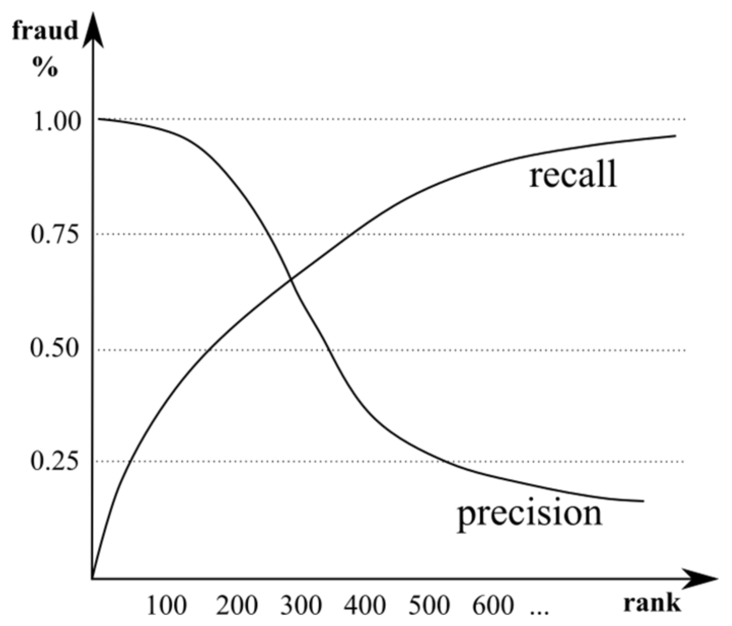
2.6. Performance Measures
2.7. Model Algorithm Selection
3. Related Work
4. Experiment
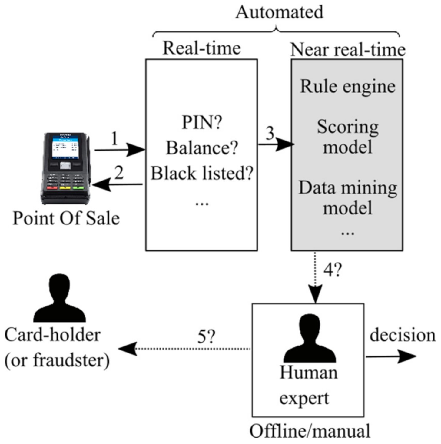
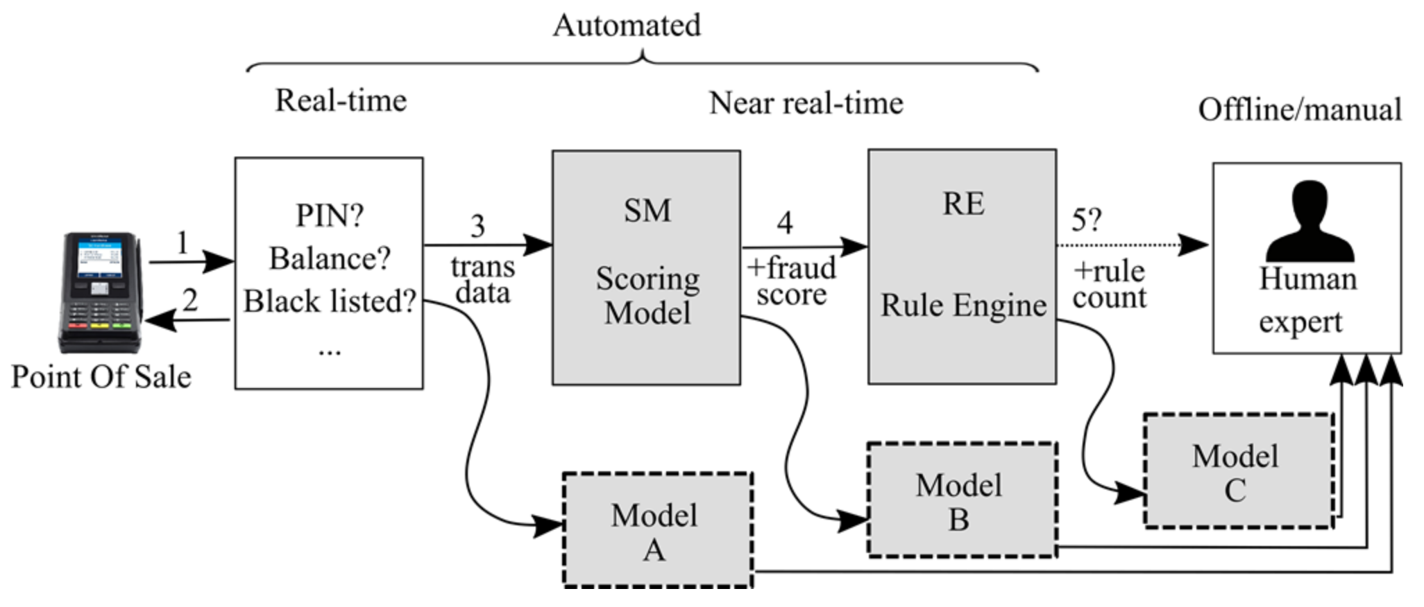
4.1. Baseline System
- Position A: parallel to the SM;
- Position B: parallel to RE, with the model being aware of the fraud score; and
- Position C: after the rule engine, with the model being aware of the rule count.
4.2. Dataset and Experiment Setup
- 66 are transaction features;
- 305 are aggregated features computed from the card’s previous transactions. For instance, one variable is “the number of ATM transactions in the past 30 days”. Current models use only eight aggregated features, and we have aggressively expanded the feature set to evaluate the aggregated features’ impact on the model quality. It should be noted that aggregated features are not free of cost—they incur significant resource costs: to calculate them in near real-time, one must have transaction history at their disposal for fast computation of features. Keeping that in mind, the transaction rate of credit card processing can be quite a technological challenge;
- Depending on the model position, fraud_score and rule_count features are available to models B and C; and
- Target variable: whether a transaction is a fraud or not.
- For the model training purposes, the dataset was divided into training and test datasets:
- Training dataset: 70% of transactions, roughly first two months.
- Test dataset: 30% of transactions, roughly the third month.
- Model position: A, B, or C.
- Fraud percentage: 5% or 50%. The latter is obtained in two ways:
- ○
- Undersampling of the majority class while preserving all fraud transactions—the resulting dataset has ~14 k transactions and is referred to as “small”.
- ○
- Combination of undersampling and oversampling—the resulting dataset has ~120 k transactions and is referred to as “balanced”.
- Basic (transactional) set of 66 features and the full set of features. The former is here referred to as “trans”.
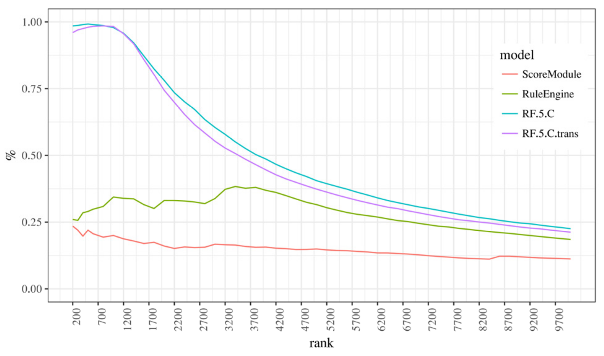
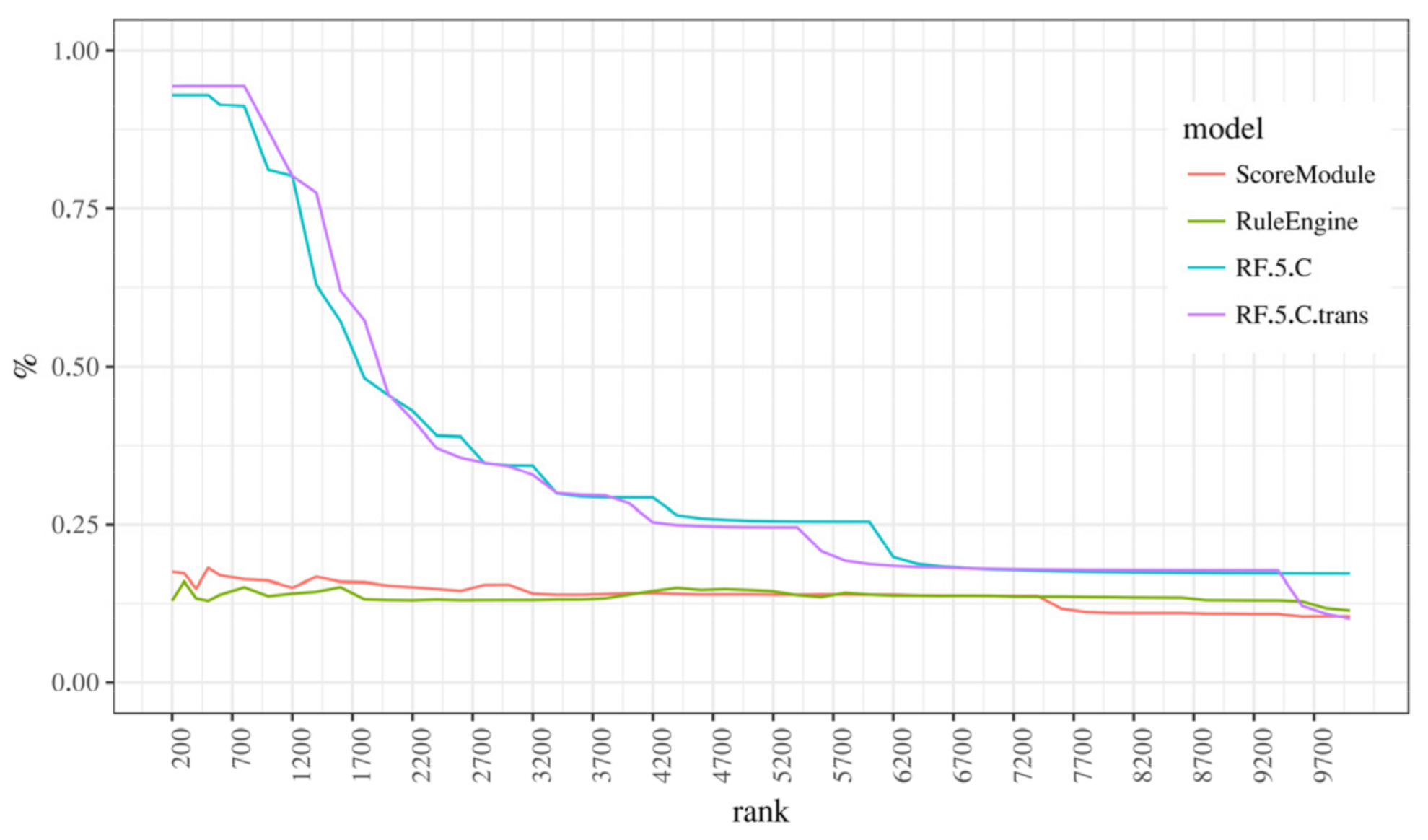
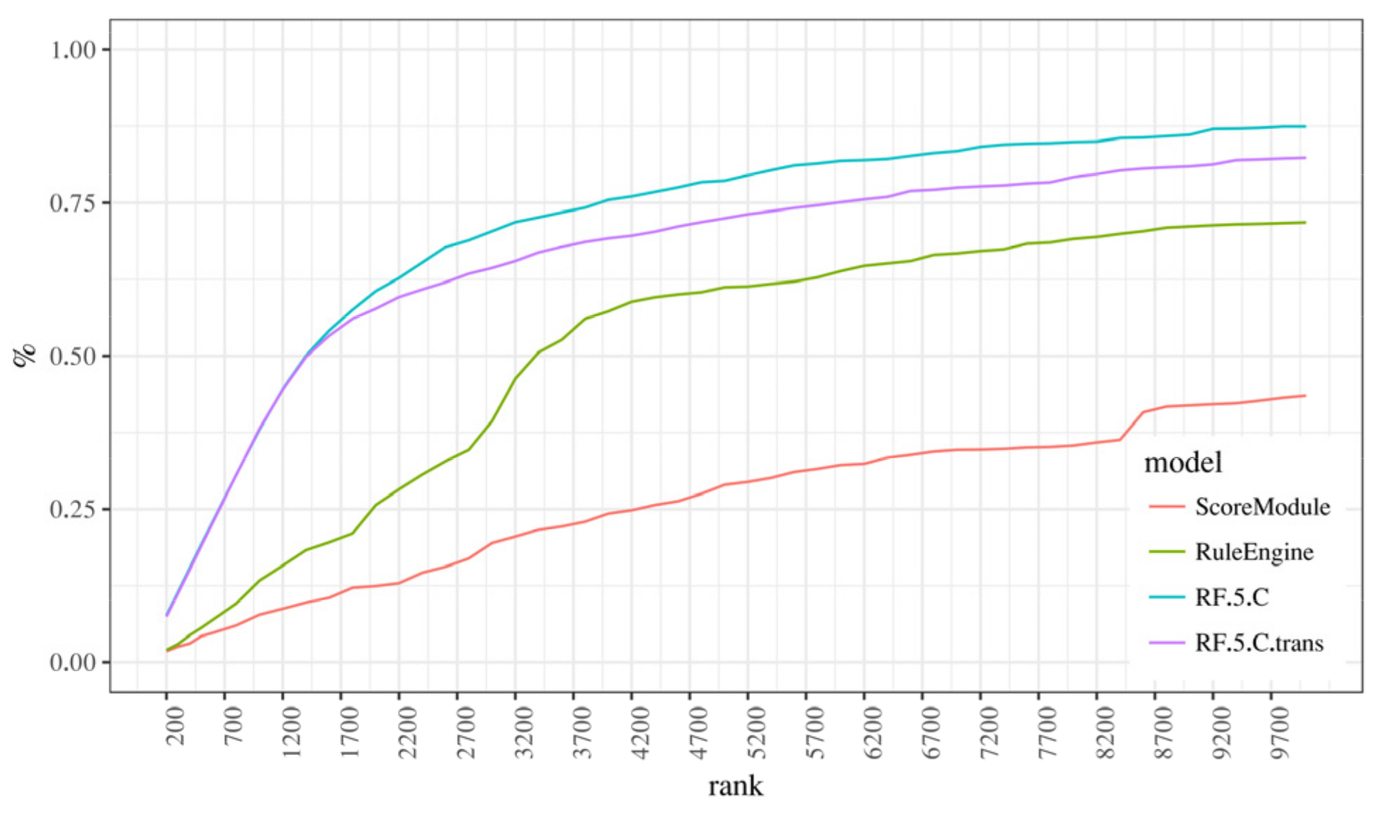
4.3. Performance Measures
5. Methodology
- Logistic regression (LR)—we used the L1 regularization and considered the regularization constant as a hyperparameter. This linear model is similar to the SM model.
- Multilayer perceptron (MLP)—is a fully connected neural network with one hidden layer. This model’s advantage over the LR model is that it produces a nonlinear mapping from inputs to outputs. Thus, it may be able to better capture more complex interactions between input variables, which could lead to more accurate predictions. However, this model’s nonlinear nature makes it much more prone to overfitting, which might offset the mentioned advantages. We used minibatch backpropagation to train the model. For regularization, we used dropout [67] and experimented with different numbers of neurons in the hidden layer (see Table 2 for details).
- Random forest (RF)—is an ensemble of decision trees learned on different feature and data subsets. This model is nonlinear and relatively robust to overfitting. This model’s additional advantages are its short training time and a degree of interpretability of model decisions. Relevant hyperparameters were the minimal size of a tree node and the number of variables to possibly split at each node.
5.1. Scaling Input Data
5.2. Feature Selection
5.3. Classifiers Comparison
5.4. Richer Features vs. More Complex Models
- How large is the difference between the baseline RE model and the developed models?
- How much performance is gained by switching from a linear to a nonlinear model?
- How much performance can be gained by including aggregated features in addition to trans features?
6. On Aggregated Features and Weighted Measures
7. Discussion
8. Conclusions
Author Contributions
Funding
Institutional Review Board Statement
Informed Consent Statement
Data Availability Statement
Acknowledgments
Conflicts of Interest
References
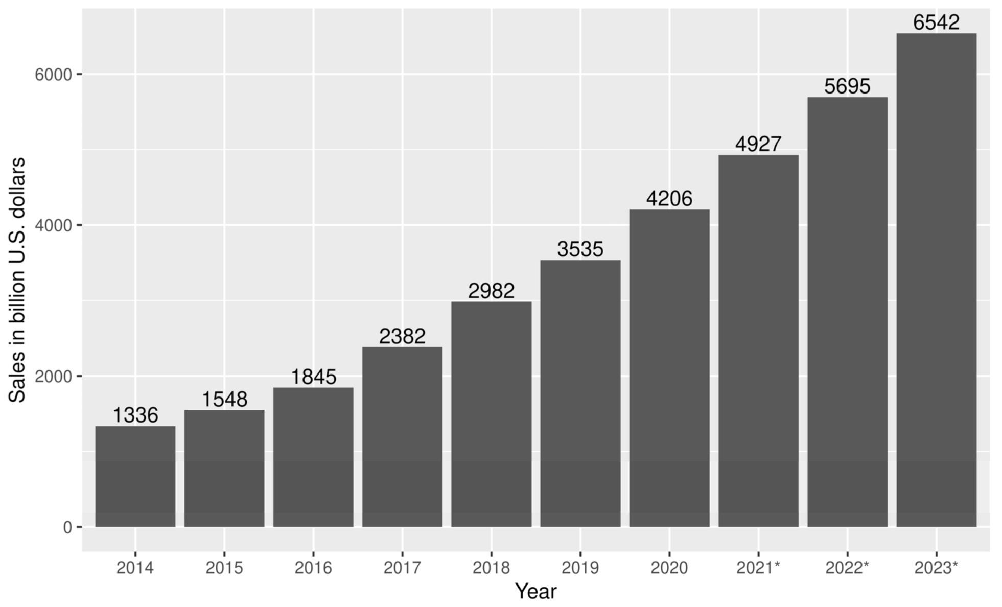
- Statista Retail e-Commerce Sales Worldwide from 2014 to 2023 (in Billion U.S. Dollars). Available online: https://www.statista.com/statistics/379046/worldwide-retail-e-commerce-sales/ (accessed on 30 September 2020).
- Statista Value of Annual Losses on “Card-Not Present” Fraud on UK-Issued Debit and Credit Cards in the United Kingdom (UK) from 2002 to 2019. Available online: https://www.statista.com/statistics/286245/united-kingdom-uk-card-not-present-fraud-losses/ (accessed on 30 September 2020).
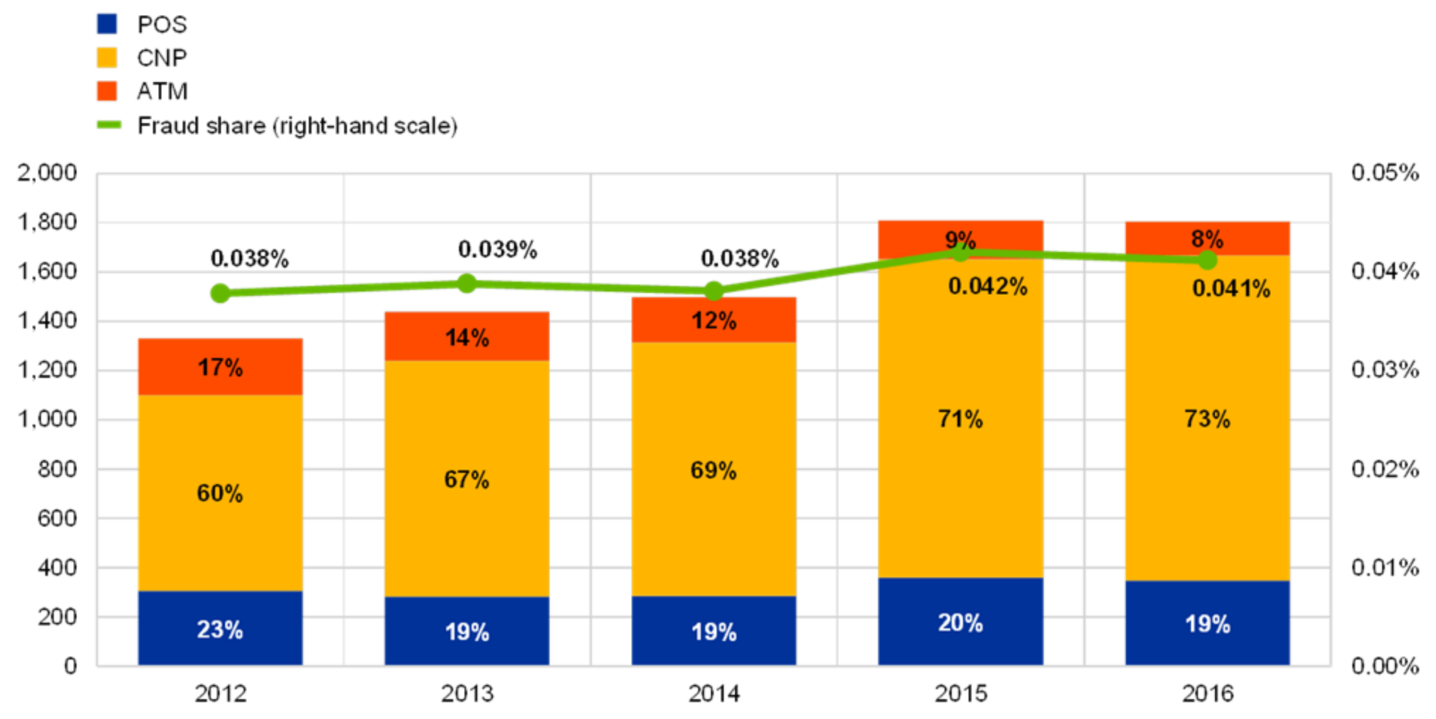
- Bank, E.C. Sixth Report on Card Fraud, August 2020; European Central Bank: Frankfurt, Germany, 2020. [Google Scholar]
- Mekterović, I.; Brkić, L.; Baranović, M. A Systematic Review of Data Mining Approaches to Credit Card Fraud Detection. WSEAS Trans. Bus. Econ. 2018, 15, 437–444. [Google Scholar]
- Priscilla, C.V.; Prabha, D.P. Credit Card Fraud Detection: A Systematic Review. In Intelligent Computing Paradigm and Cutting-edge Technologies, Proceedings of the First International Conference on Innovative Computing and Cutting-Edge Technologies (ICICCT 2019), Istanbul, Turkey, 30–31 October 2019; Springer: Cham, Switzerland, 2019; pp. 290–303. [Google Scholar] [CrossRef]
- Găbudeanu, L.; Brici, I.; Mare, C.; Mihai, I.C.; Șcheau, M.C. Privacy Intrusiveness in Financial-Banking Fraud Detection. Risks 2021, 9, 104. [Google Scholar] [CrossRef]
- Zakaryazad, A.; Duman, E. A profit-driven Artificial Neural Network (ANN) with applications to fraud detection and direct marketing. Neurocomputing 2016, 175, 121–131. [Google Scholar] [CrossRef]
- Robinson, W.N.; Aria, A. Sequential fraud detection for prepaid cards using hidden Markov model divergence. Expert Syst. Appl. 2018, 91, 235–251. [Google Scholar] [CrossRef]
- Khalilia, M.; Chakraborty, S.; Popescu, M. Predicting disease risks from highly imbalanced data using random forest. BMC Med. Inform. Decis. Mak. 2011, 11, 51. [Google Scholar] [CrossRef] [PubMed] [Green Version]
- Sharifai, G.A.; Zainol, Z. Feature selection for high-dimensional and imbalanced biomedical data based on robust correlation based redundancy and binary grasshopper optimization algorithm. Genes 2020, 11, 717. [Google Scholar] [CrossRef]
- Huang, C.; Li, Y.; Change Loy, C.; Tang, X. Deep Imbalanced Learning for Face Recognition and Attribute Prediction. IEEE Trans. Pattern Anal. Mach. Intell. 2020, 42, 2781–2794. [Google Scholar] [CrossRef] [PubMed] [Green Version]
- Ngo, Q.T.; Yoon, S. Facial Expression Recognition Based on Weighted-Cluster Loss and Deep Transfer Learning Using a Highly Imbalanced Dataset. Sensors 2020, 20, 2639. [Google Scholar] [CrossRef]
- Kubat, M.; Holte, R.C.; Matwin, S.; Kohavi, R.; Provost, F. Machine Learning for the Detection of Oil Spills in Satellite Radar Images. Mach. Learn. 1998, 30, 195–215. [Google Scholar] [CrossRef] [Green Version]
- Ouyang, X.; Chen, Y.; Wei, B. Experimental Study on Class Imbalance Problem Using an Oil Spill Training Data Set. J. Adv. Math. Comput. Sci. 2017, 21, 1–9. [Google Scholar] [CrossRef]
- Fernández-Gómez, M.J.; Asencio-Cortés, G.; Troncoso, A.; Martínez-álvarez, F. Large earthquake magnitude prediction in Chile with imbalanced classifiers and ensemble learning. Appl. Sci. 2017, 7, 625. [Google Scholar] [CrossRef] [Green Version]
- Bermejo, P.; Gámez, J.A.; Puerta, J.M. Improving the performance of Naive Bayes multinomial in e-mail foldering by introducing distribution-based balance of datasets. Expert Syst. Appl. 2011, 38, 2072–2080. [Google Scholar] [CrossRef]
- Lin, W.; Wu, Z.; Lin, L.; Wen, A.; Li, J. An ensemble random forest algorithm for insurance big data analysis. IEEE Access 2017, 5, 16568–16575. [Google Scholar] [CrossRef]
- Dal Pozzolo, A. Adaptive Machine Learning for Credit Card Fraud Detection Declaration of Authorship. Ph.D. Thesis, Université Libre de Bruxelles, Brussels, Belgium, December 2015; p. 199. [Google Scholar]
- Chawla, N.; Bowyer, K. SMOTE: Synthetic Minority Over-sampling Technique Nitesh. J. Artif. Intell. Res. 2002, 16, 321–357. [Google Scholar] [CrossRef]
- Chawla, N.V.; Lazarevic, A.; Hall, L.O.; Bowyer, K.W. SMOTEBoost: Improving prediction of the minority class in boosting. In Knowledge Discovery in Databases: PKDD 2003; Springer: Berlin/Heidelberg, Germany, 2003; Volume 2838, pp. 107–119. [Google Scholar] [CrossRef] [Green Version]
- Liu, X.Y.; Wu, J.; Zhou, Z.H. Exploratory under-sampling for class-imbalance learning. IEEE Trans. Syst. Man Cybern. Part B Cybern. 2008, 39, 539–550. [Google Scholar] [CrossRef]
- Yen, S.-J.; Lee, Y.-S. Cluster-based under-sampling approaches for imbalanced data distributions. Expert Syst. Appl. 2009, 36, 5718–5727. [Google Scholar] [CrossRef]
- Hanifah, F.S.; Wijayanto, H.; Kurnia, A. SMOTE bagging algorithm for imbalanced dataset in logistic regression analysis (case: Credit of bank X). Appl. Math. Sci. 2015, 9, 6857–6865. [Google Scholar] [CrossRef] [Green Version]
- Zhou, Z.H.; Liu, X.Y. Training cost-sensitive neural networks with methods addressing the class imbalance problem. IEEE Trans. Knowl. Data Eng. 2006, 18, 63–77. [Google Scholar] [CrossRef]
- Thai-Nghe, N.; Gantner, Z.; Schmidt-Thieme, L. Cost-sensitive learning methods for imbalanced data. In Proceedings of the 2010 International Joint Conference on Neural Networks (IJCNN), Barcelona, Spain, 18–23 July 2010; pp. 1–8. [Google Scholar] [CrossRef] [Green Version]
- Kubat, M.; Widmer, G. Adapting to drift in continuous domains. In Machine Learning: ECML-95, Proceedings of the 8th European Conference on Machine Learning Heraclion, Crete, Greece, 25–27 April 1995; Springer: Berlin/Heidelberg, Germany, 1995; pp. 307–310. [Google Scholar]
- Barros, R.S.M.; Cabral, D.R.L.; Gonçalves, P.M.; Santos, S.G.T.C. RDDM: Reactive drift detection method. Expert Syst. Appl. 2017, 90, 344–355. [Google Scholar] [CrossRef]
- de Lima Cabral, D.R.; de Barros, R.S.M. Concept drift detection based on Fisher’s Exact test. Inf. Sci. 2018, 442–443, 220–234. [Google Scholar] [CrossRef]
- Yu, S.; Abraham, Z.; Wang, H.; Shah, M.; Wei, Y.; Príncipe, J.C. Concept drift detection and adaptation with hierarchical hypothesis testing. J. Franklin Inst. 2019, 356, 3187–3215. [Google Scholar] [CrossRef] [Green Version]
- Liu, G.; Cheng, H.R.; Qin, Z.G.; Liu, Q.; Liu, C.X. E-CVFDT: An improving CVFDT method for concept drift data stream. In Proceedings of the 2013 International Conference on Communications, Circuits and Systems (ICCCAS), Chengdu, China, 15–17 November 2013; Volume 1, pp. 315–318. [Google Scholar]
- Bifet, A.; Gavaldà, R. Learning from Time-Changing Data with Adaptive Windowing *. In Proceedings of the 2007 SIAM International Conference on Data Mining (SDM), Minneapolis, MN, USA, 26–28 April 2007. [Google Scholar]
- Haque, A.; Khan, L.; Baron, M.; Thuraisingham, B.; Aggarwal, C. Efficient handling of concept drift and concept evolution over Stream Data. In Proceedings of the 2016 IEEE 32nd International Conference on Data Engineering (ICDE), Helsinki, Finland, 16–20 May 2016; pp. 481–492. [Google Scholar]
- Ditzler, G.; Polikar, R. Incremental learning of concept drift from streaming imbalanced data. IEEE Trans. Knowl. Data Eng. 2013, 25, 2283–2301. [Google Scholar] [CrossRef]
- Brzeziński, D.; Stefanowski, J. Accuracy updated ensemble for data streams with concept drift. In Lecture Notes in Computer Science (Including Subseries Lecture Notes in Artificial Intelligence and Lecture Notes in Bioinformatics); Springer: Berlin/Heidelberg, Germany, 2011; Volume 6679, pp. 155–163. [Google Scholar]
- Gama, J.; Zliobaite, I.; Bifet, A.; Pechenizkiy, M.; Bouchachia, A. A survey on concept drift adaptation. ACM Comput. Surv. 2014, 46, 1–37. [Google Scholar] [CrossRef]
- Wares, S.; Isaacs, J.; Elyan, E. Data stream mining: Methods and challenges for handling concept drift. SN Appl. Sci. 2019, 1, 1412. [Google Scholar] [CrossRef] [Green Version]
- Tsymbal, A. The problem of concept drift: Definitions and related work. Comput. Sci. Dep. Trinity Coll. Dublin 2004, 106, 58. [Google Scholar]
- Leonard, K.J. The development of a rule based expert system model for fraud alert in consumer credit. Eur. J. Oper. Res. 1995, 80, 350–356. [Google Scholar] [CrossRef]
- Gianini, G.; Ghemmogne Fossi, L.; Mio, C.; Caelen, O.; Brunie, L.; Damiani, E. Managing a pool of rules for credit card fraud detection by a Game Theory based approach. Futur. Gener. Comput. Syst. 2020, 102, 549–561. [Google Scholar] [CrossRef]
- Bolton, R.J.; Hand, D.J. Unsupervised Profiling Methods for Fraud Detection. Proc. Credit Scoring Credit Control 2001, VII, 5–7. [Google Scholar]
- Bahnsen, A.C.; Stojanovic, A.; Aouada, D.; Ottersten, B. Cost sensitive credit card fraud detection using bayes minimum risk. In Proceedings of the 2013 12th International Conference on Machine Learning and Applications, Miami, FL, USA, 4–7 December 2013; Volume 1, pp. 333–338. [Google Scholar] [CrossRef]
- Huang, J.; Zhu, Q.; Yang, L.; Cheng, D.D.; Wu, Q. A novel outlier cluster detection algorithm without top-n parameter. Knowl. Based Syst. 2017, 121, 32–40. [Google Scholar] [CrossRef]
- Thakran, Y.; Toshniwal, D. Unsupervised outlier detection in streaming data using weighted clustering. In Proceedings of the 2012 12th International Conference on Intelligent Systems Design and Applications (ISDA), Kochi, India, 27–29 November 2012; pp. 947–952. [Google Scholar] [CrossRef] [Green Version]
- Koufakou, A.; Secretan, J.; Georgiopoulos, M. Non-derivable itemsets for fast outlier detection in large high-dimensional categorical data. Knowl. Inf. Syst. 2011, 29, 697–725. [Google Scholar] [CrossRef]
- Dorronsoro, J.R.; Ginel, F.; Sánchez, C.; Santa Cruz, C. Neural fraud detection in credit card operations. IEEE Trans. Neural Netw. 1997, 8, 827–834. [Google Scholar] [CrossRef] [PubMed] [Green Version]
- Ghosh, S.; Reilly, D.L. Credit card fraud detection with a neural-network. In Proceedings of the Twenty-Seventh Hawaii International Conference on System Sciences, Wailea, HI, USA, 4–7 January 1994; Volume 3, pp. 621–630. [Google Scholar] [CrossRef]
- Gómez, J.A.; Arévalo, J.; Paredes, R.; Nin, J. End-to-end neural network architecture for fraud scoring in card payments. Pattern Recognit. Lett. 2018, 105, 175–181. [Google Scholar] [CrossRef]
- Jurgovsky, J.; Granitzer, M.; Ziegler, K.; Calabretto, S.; Portier, P.E.; He-Guelton, L.; Caelen, O. Sequence classification for credit-card fraud detection. Expert Syst. Appl. 2018, 100, 234–245. [Google Scholar] [CrossRef]
- Whitrow, C.; Hand, D.J.; Juszczak, P.; Weston, D.; Adams, N.M. Transaction aggregation as a strategy for credit card fraud detection. Data Min. Knowl. Discov. 2009, 18, 30–55. [Google Scholar] [CrossRef]
- Bhattacharyya, S.; Jha, S.; Tharakunnel, K.; Westland, J.C. Data mining for credit card fraud: A comparative study. Decis. Support Syst. 2011, 50, 602–613. [Google Scholar] [CrossRef]
- Ravisankar, P.; Ravi, V.; Raghava Rao, G.; Bose, I. Detection of financial statement fraud and feature selection using data mining techniques. Decis. Support Syst. 2011, 50, 491–500. [Google Scholar] [CrossRef]
- Jha, S.; Guillen, M.; Christopher Westland, J. Employing transaction aggregation strategy to detect credit card fraud. Expert Syst. Appl. 2012, 39, 12650–12657. [Google Scholar] [CrossRef]
- Correa Bahnsen, A.; Aouada, D.; Stojanovic, A.; Ottersten, B. Feature engineering strategies for credit card fraud detection. Expert Syst. Appl. 2016, 51, 134–142. [Google Scholar] [CrossRef]
- Randhawa, K.; Loo, C.K.; Seera, M.; Lim, C.P.; Nandi, A.K. Credit Card Fraud Detection Using AdaBoost and Majority Voting. IEEE Access 2018, 6, 14277–14284. [Google Scholar] [CrossRef]
- Dal Pozzolo, A.; Boracchi, G.; Caelen, O.; Alippi, C.; Bontempi, G. Credit card fraud detection and concept-drift adaptation with delayed supervised information. In Proceedings of the 2015 International Joint Conference on Neural Networks (IJCNN), Killarney, Ireland, 12–17 July 2015. [Google Scholar] [CrossRef]
- Bahnsen, A.C.; Aouada, D.; Ottersten, B. Example-dependent cost-sensitive decision trees. Expert Syst. Appl. 2015, 42, 6609–6619. [Google Scholar] [CrossRef]
- Mahmoudi, N.; Duman, E. Detecting credit card fraud by Modified Fisher Discriminant Analysis. Expert Syst. Appl. 2015, 42, 2510–2516. [Google Scholar] [CrossRef]
- Kültür, Y.; Çağlayan, M.U. Hybrid approaches for detecting credit card fraud. Expert Syst. 2017, 34, 1–13. [Google Scholar] [CrossRef]
- Askari, S.M.S.; Hussain, M.A. IFDTC4.5: Intuitionistic fuzzy logic based decision tree for E-transactional fraud detection. J. Inf. Secur. Appl. 2020, 52, 102469. [Google Scholar] [CrossRef]
- Ryman-Tubb, N.F.; Krause, P. Neural network rule extraction to detect credit card fraud. In Engineering Applications of Neural Networks, Proceedings of the 12th INNS EANN-SIG International Conference, EANN 2011 and 7th IFIP WG 12.5 International Conference, AIAI 2011, Corfu, Greece, 15–18 September 2011; Volume 363, pp. 101–110. [CrossRef] [Green Version]
- Sánchez, D.; Vila, M.A.; Cerda, L.; Serrano, J.M. Association rules applied to credit card fraud detection. Expert Syst. Appl. 2009, 36, 3630–3640. [Google Scholar] [CrossRef]
- How Artificial Intelligence Could Stop Those Awkward Moments When Your Credit Card Is Mistakenly Declined—The Washington Post. Available online: https://www.washingtonpost.com/news/innovations/wp/2016/12/02/how-ai-could-stop-those-awkward-moments-when-your-credit-card-is-mistakenly-declined (accessed on 7 December 2020).
- LogSentinel. Available online: https://logsentinel.com/ (accessed on 1 March 2020).
- Panigrahi, S.; Kundu, A.; Sural, S.; Majumdar, A.K. Credit card fraud detection: A fusion approach using Dempster-Shafer theory and Bayesian learning. Inf. Fusion 2009, 10, 354–363. [Google Scholar] [CrossRef]
- Turpin, A.; Scholer, F. User performance versus precision measures for simple search tasks. In Proceedings of the Twenty-Ninth Annual International ACM SIGIR Conference on Research and Development in Information Retrieval, Seattle, WA, USA, 6–11 August 2006; Association for Computing Machinery (ACM): New York, NY, USA, 2006; Volume 2006, pp. 11–18. [Google Scholar]
- Dal Pozzolo, A.; Caelen, O.; Le Borgne, Y.A.; Waterschoot, S.; Bontempi, G. Learned lessons in credit card fraud detection from a practitioner perspective. Expert Syst. Appl. 2014, 41, 4915–4928. [Google Scholar] [CrossRef]
- Srivastava, N.; Hinton, G.; Krizhevsky, A.; Salakhutdinov, R. Dropout: A Simple Way to Prevent Neural Networks from Overfitting. J. Mach. Learn. Res. 2014, 15, 929–1958. [Google Scholar]
- Hoens, T.R.; Polikar, R.; Chawla, N.V. Learning from streaming data with concept drift and imbalance: An overview. Prog. Artif. Intell. 2012, 1, 89–101. [Google Scholar] [CrossRef] [Green Version]
- Carcillo, F.; Dal Pozzolo, A.; Le Borgne, Y.A.; Caelen, O.; Mazzer, Y.; Bontempi, G. SCARFF: A scalable framework for streaming credit card fraud detection with spark. Inf. Fusion 2018, 41, 182–194. [Google Scholar] [CrossRef] [Green Version]


| Abbreviation | Meaning |
|---|---|
| trans | Only basic (transactional) set of 66 features. If omitted, full feature set, which includes aggregated features, is used. |
| 5 | 5% fraud rate |
| 50 | 50% fraud rate |
| {small|balance} | small is obtained through undersampling of majority class and balanced with a combination of undersampling and oversampling. If none of these appears, then the integral dataset has been used. |
| A, B, C | Model position, see Figure 4 |
| RF, LR, or NN | random forest, logistic regression, or neural network, respectively |
| Classifier | Hyperparameter | Values |
|---|---|---|
| LR | cost | 0.001, 0.001, 0.01, 0.1, 1, 100 |
| LR | regularization term in the loss | L1, L2 |
| MLP | number of neurons | 10, 20, 30 |
| RF | number of trees | 15, 20, 25 |
| RF | minimal node size | 10, 15, 20 |
| Classifier | Recall | Precision | F1 | AP |
|---|---|---|---|---|
| Baseline (RE) | 0.564 | 0.379 | 0.453 | 0.189 |
| LR without scaling | 0.806 | 0.255 | 0.387 | 0.472 |
| LR with scaling | 0.802 | 0.255 | 0.386 | 0.473 |
| RF without scaling | 0.835 | 0.370 | 0.514 | 0.697 |
| RF with scaling | 0.840 | 0.367 | 0.512 | 0.695 |
| Classifier | Recall | Precision | F1 | AP |
|---|---|---|---|---|
| Baseline (RE) | 0.564 | 0.379 | 0.453 | 0.189 |
| LR with 30 features | 0.818 | 0.205 | 0.327 | 0.311 |
| LR with 100 features | 0.813 | 0.230 | 0.359 | 0.429 |
| LR with all features | 0.803 | 0.254 | 0.586 | 0.472 |
| RF with 30 features | 0.846 | 0.338 | 0.483 | 0.709 |
| RF with 100 features | 0.853 | 0.357 | 0.504 | 0.725 |
| RF with all features | 0.836 | 0.371 | 0.514 | 0.696 |
| Classifier | Recall | Precision | F1 | AP |
|---|---|---|---|---|
| Baseline (RE) | 0.564 | 0.378 | 0.453 | 0.189 |
| LR.5.A.sm | 0.454 | 0.766 | 0.570 | 0.388 |
| LR.5.B.sm | 0.454 | 0.763 | 0.569 | 0.387 |
| LR.5.C.sm | 0.451 | 0.759 | 0.566 | 0.385 |
| MLP.5.A.sm | 0.454 | 0.786 | 0.576 | 0.393 |
| MLP.5.B.sm | 0.441 | 0.707 | 0.543 | 0.354 |
| MLP.5.C.sm | 0.464 | 0.739 | 0.570 | 0.391 |
| RF.5.A.sm | 0.517 | 0.932 | 0.665 | 0.512 |
| RF.5.B.sm | 0.517 | 0.932 | 0.665 | 0.512 |
| RF.5.C.sm | 0.519 | 0.934 | 0.667 | 0.515 |
| Classifier | Recall | Precision | F1 | AP |
|---|---|---|---|---|
| Baseline (RE) | 0.564 | 0.378 | 0.453 | 0.189 |
| LR.5.C.sm | 0.451 | 0.759 | 0.566 | 0.385 |
| LR.5.C.sm.trans | 0.375 | 0.749 | 0.500 | 0.308 |
| RF.5.C.sm | 0.519 | 0.934 | 0.667 | 0.515 |
| RF.5.C.sm.trans | 0.411 | 0.893 | 0.563 | 0.399 |
Publisher’s Note: MDPI stays neutral with regard to jurisdictional claims in published maps and institutional affiliations. |
© 2021 by the authors. Licensee MDPI, Basel, Switzerland. This article is an open access article distributed under the terms and conditions of the Creative Commons Attribution (CC BY) license (https://creativecommons.org/licenses/by/4.0/).
Share and Cite
Mekterović, I.; Karan, M.; Pintar, D.; Brkić, L. Credit Card Fraud Detection in Card-Not-Present Transactions: Where to Invest? Appl. Sci. 2021, 11, 6766. https://doi.org/10.3390/app11156766
Mekterović I, Karan M, Pintar D, Brkić L. Credit Card Fraud Detection in Card-Not-Present Transactions: Where to Invest? Applied Sciences. 2021; 11(15):6766. https://doi.org/10.3390/app11156766
Chicago/Turabian StyleMekterović, Igor, Mladen Karan, Damir Pintar, and Ljiljana Brkić. 2021. "Credit Card Fraud Detection in Card-Not-Present Transactions: Where to Invest?" Applied Sciences 11, no. 15: 6766. https://doi.org/10.3390/app11156766
APA StyleMekterović, I., Karan, M., Pintar, D., & Brkić, L. (2021). Credit Card Fraud Detection in Card-Not-Present Transactions: Where to Invest? Applied Sciences, 11(15), 6766. https://doi.org/10.3390/app11156766