Abstract
As reported in the recent image velocimetry literature, tracking the motion of sparse feature points floating on the river surface as done by the Optical Tracking Velocimetry (OTV) algorithm is a promising strategy to address surface flow monitoring. Moreover, the lightweight nature of OTV coupled with computational optimizations makes it suited even for its deployment in situ to perform measurements at the edge with cheap embedded devices without the need to perform offload processing. Despite these notable achievements, the actual practical deployment of OTV in remote environments would require cheap and self-powered systems enabling continuous measurements without the need for cumbersome and expensive infrastructures rarely found in situ. Purposely, in this paper, we propose an additional simplification to the OTV algorithm to reduce even further its computational requirements, and we analyze self-powered off-the-shelf setups for in situ deployment. We assess the performance of such set-ups from different perspectives to determine the optimal solution to design a cost-effective self-powered measurement node.
1. Introduction
Surface flow monitoring from images is a promising yet well-known technique to face the problem of estimating river flow velocity. River velocity measurements typically require relevant human and financial efforts for organizing sporadic campaigns that, in addition, cannot be carried out, for safety reasons, during flood events, when such information is more vital. Therefore, automatic measuring systems are pivotal to avoid cumbersomely demanding and expensive procedures carried out by specialized human operators. Radar systems are still costly and cannot monitor the entire width of medium-large rivers. Conversely, automatic image-based methods would seamlessly enable continuous monitoring with clear advantages, among many, for costs and for the frequency and spatial density of measurements in case multiple devices are deployed along the river.
In open channels, streamflow monitoring is typically conducted through the velocity-area method, which is based on discrete integration of discharge from flow velocity and depth measurements sampled throughout the channel cross section. This mandates the use of permanent installations of instrumentation powered through the grid. For instance, acoustic Doppler current profilers (ADCPs), pulsed doppler radars, and ultrasonic water level meters are among the most popular systems for streamflow measurements. In recent years, several research groups have been investigating on innovative monitoring approaches with image analysis, and some companies have been providing off-the-shelf image-based systems for river flow monitoring (www.tenevia.com, accessed on 28 July 2021, www.photrack.ch, accessed on 28 July 2021). However, a thorough assessment of the power consumption characteristics of such systems is not available. Furthermore, commercially-available systems exploit proprietary software, and involve centralized supervisors at the companies to store and manage data.
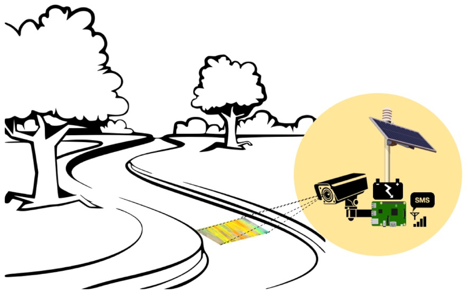
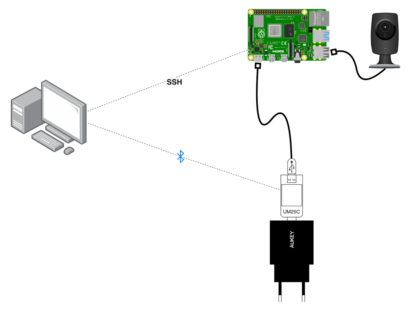
For the reasons outlined, this topic has been deeply investigated in the literature, and the Optical Tracking Velocimetry (Source code available at: https://github.com/fabiotosi92/Optical-Tracking-Velocimetry, accessed on 28 July 2021) technique [1] seems particularly promising. This technique allows for achieving state-of-the-art results in a fraction of the time required by other methods without the need for wideband communication infrastructures for off-load processing. Moreover, its lightweight computational structure also enables deployment on standard and cheap embedded devices such as those belonging to the Raspberry Pi family [2], as reported in [3]. Therefore, it appears at hand the opportunity to design cheap and self-powered monitoring systems capable of continuous monitoring in situ without any constraint regarding the available infrastructures as sketched in Figure 1. It is worth highlighting that, with such a configuration, a simple low bandwidth text messaging system would suffice to communicate to a centralized server the outcome of the velocity estimation procedure, with a simple SMS, instead of transmitting the entire, heavy images to be then processed elsewhere, with significant implications concerning cost and scalability if a distributed network of gauge-cameras is deployed.

Figure 1.
Sketch of the envisioned solar-powered measurement node made up of standard off-the-shelf devices placed in a remote monitoring site. The outcome computed in situ by the node is optionally sent to a centralized gathering system through standard text messaging such as a simple SMS requiring a shallow bandwidth communication channel.
With this goal in mind, in this paper, at first, we propose an additional simplification to the OTV algorithm to reduce further its computational requirements without sacrificing its accuracy. Then, we define some self-powered setups based on cheap and standard solar panels and computing devices available on the market, and evaluate their performance to obtain the best trade-off between cost and measurement rate. Specifically, we analyze the raw performance of the OTV algorithm on each platform, with different architectures and optimization strategies, and assess overall energy consumption to evaluate the measurement rate with rechargeable batteries coupled with small solar panels. A particularly appealing setup would consist of cheap off-the-shelf components such as a standard RGB or monochrome camera, and a Raspberry Pi powered by a PJuice Hat consisting of a lithium battery rechargeable by a small solar panel. The overall cost of a similar setup would be only a few hundred dollars, thus affording its capillary deployment even in developing countries. Optionally, when continuous reporting is needed, such a setup could include a SIM-based text messaging system connected to the Raspberry Pi and powered by the same rechargeable battery previously mentioned.
Indeed, the thorough analysis carried out in this paper highlights that practical continuous surface flow monitoring in situ, even in remote places far from urban areas, is feasible with cheap off-the-shelf components. This paves the way for such an automatic capillary measurement methodology to be applied in countless monitoring sites.
2. Related Work
In the past few years, automatic image velocimetry methodologies for river monitoring have blossomed [4]. Most of such approaches stem from traditional large scale particle image velocimetry (LSPIV) [5], particle tracking velocimetry (PTV) [6], optical flow [7], and exhibit diverse sensitivity to flow regime and seeding density. The OTV approach combines automated feature detection, tracking through the Lucas–Kanade algorithm, and trajectory-based filtering that retain the most realistic trajectories which pertain to objects transiting in the field of view [1]. Features such as corners and junctions are detected through the Fast from Accelerated Segment Test (FAST) algorithm. Such features are then tracked with the pyramidal Lucas–Kanade sparse first-order differential technique. Images are sub-sampled up to four levels, and out of all trajectories, only those which exhibit a minimum length and inclination with respect to the stream cross-section are retained for further processing. OTV does not rely on the deployment of tracers in the field of view, and the length and angle of the trajectory need to be defined by the user, as well as the maximum number of trajectories. The method works well in conditions where surface features are sparse, and where flows are unsteady [1]. Recently, OTV has been optimized by leveraging its parallel processing capability to facilitate in situ deployment [3].
Similar methodologies include the KLT-IV v1.0 that offers a user-friendly graphical interface for the determination of river flow velocity and river discharge using videos acquired from a variety of fixed and mobile platforms [8]. Likewise, the Surface Structure Image Velocimetry (SSIV) uses a cross-correlation algorithm similar to LSPIV and further introduces a filter which mitigates the effects of shadows and glare as well as the need for a densely seeded flow surface [9]. While the SSIV commercial software is available as a smartphone app and for permanent monitoring implementations, self-powered setups featuring automatic surface flow velocity measurement at the edge in remote environments are still untapped. In this vein, the OpenRiverCam initiative is an open-source and low cost web-software stack with API to establish and maintain river rating curves in small to medium sized streams based on LSPIV [10]. Further initiatives aimed at creating a network of monitoring stations for streamflow monitoring include [11], where simple camera setups enable water level estimations in the upland area of a headwater river basin.
3. Fast Optical Tracking Velocimetry
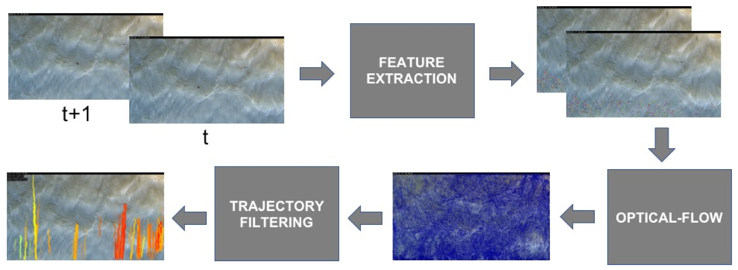
Due to its relevant practical applications, surface flow monitoring has been deeply investigated in the past few years, and a recent trend proposes to tackle this task leveraging image feature correspondences. In this field, the OTV algorithm [1] relied on the pyramidal Lucas–Kanade algorithm [7] to track efficiently lightweight image features, such as FAST [12], extracted from consecutive frames of a video stream, as depicted in Figure 2. Specifically, given two consecutive image frames of a video sequence at time t and , it extracts relevant features (e.g., FAST [12] from them and searches for corresponding ones through the Lucas–Kanade optical-flow algorithm [7]. The outcome of this process is then processed to detect inconsistent trajectories according to priors about the expected rough river flow direction [1].
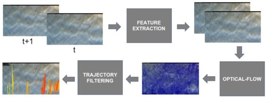
Figure 2.
Description of the OTV algorithm [1].
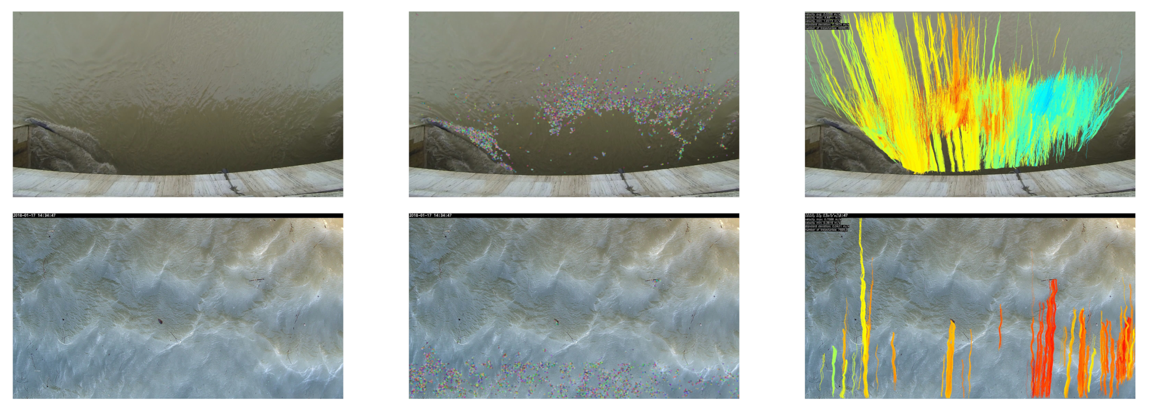
Despite its simplicity, OTV turned out quite effective compared to other methods known in the literature and much less computationally demanding. This latter feature, coupled with additional algorithmic considerations and taking advantage of accelerated computing capabilities available nowadays in almost every microprocessor systems, enabled its deployment even on low power embedded devices [3]. Figure 3 shows the outcome of the OTV algorithm processing video sequences acquired on the Tevere and Secchia rivers in Italy. The latter is particularly challenging since it frames the Secchia river during varying lighting conditions, probably originated by clouds, strongly affecting the image acquisition process. Moreover, there is also an additional perturbation generated by small waves opposite to the streamflow. Despite these multiple perturbations, OTV can reliably track a sufficient amount of features to infer streamflow behavior, as depicted in the rightmost image at the bottom of Figure 3. Nonetheless, deeper perturbations as rain and more unsatisfactory lighting conditions might degrade the capacity of OTV (as well as those of all the image velocimetry methods) to infer meaningful streamflow parameters. Although this limitation may be relevant in some cases, its analysis is out of the scope of this work. The OTV achievements potentially pave the way for surface flow monitoring at the edge. However, enabling such a task in situ, especially remote ones, requires crossing an additional hurdle concerning self-powering the overall measurement system. Purposely, in the following sections, we deeply investigate this issue using cheap solutions readily available on the market.
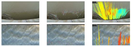
Figure 3.
(Top) a video sequence acquired on the Tevere river, (Bottom) a sequence acquired on the Secchia river; (Left) Input frame of the video sequence, (Middle) FAST features extracted from the input frame, and (Right) trajectories inferred by the OTV algorithm.
Moreover, we propose an additional optional simplification to speed up the measurement process further and potentially save energy. It simply consists of replacing color video streams with monochrome ones to reduce the most computationally intensive phase of the whole measurement process, the OTV task. As reported in the experimental results section, such a simple modification, processing images at Full and Half resolution, achieves performance substantially on-par with the original OTV approach but at a significantly faster rate, consequently draining less energy.
4. Computing Devices
With the proliferation of wearable devices, there are plenty of computing platforms suited for our purposes. Examples of such devices are the Odroid XU4 https://www.hardkernel.com/shop/odroid-xu4-special-price/ (accessed on 28 July 2021), equipped with a Samsung Exynos5422 Cortex A15 2Ghz and Cortex A7 Octa-core CPUs, and devices belonging to the Raspberry Pi family https://www.raspberrypi.org/ (accessed on 28 July 2021). These two classes of devices, such as many others available on the market, rely on ARM architectures, and, in this very case, have a very similar price, around 50$. We decided to focus on the Raspberry Pi ecosystem since it provides a wide range of cheap and power-efficient devices that would perfectly fit our aims and has a very large and active community. Specifically, we considered in our evaluation the Raspberry Pi models 3B, 3B+, and 4 (model B), all available at a very competitive price. Moreover, they have a vast community of developers worldwide and many add-ons are readily available off-the-shelf for fast prototyping. Although potentially suited for our purposes, we did not consider less powerful devices belonging to the same ecosystem, such as the Raspberry Pi Zero. Their shallow energy consumption did not seem balanced by an adequate computing performance required in the envisioned application in our preliminary analysis. All the devices considered in our experiments are equipped with the Linux operating system (Raspbian Buster).
The Raspberry Pi 3B contains Quad Core 1.2 GHz Broadcom BCM2837 64bit CPU with 1 GB DDR2 RAM memory. It also features Ethernet, wireless, Bluetooth Low Energy (BLE), four USB 2.0 ports and has, as other devices introduced next, a 40-pin GPIO connector. As for other Raspberry devices discussed next, specific functionality can be disabled through software commands to save energy.
Concerning our purposes, the Raspberry Pi model 3B+ shares very similar specifications compared to model 3B except for a higher CPU frequency (1.4 vs. 1.2 GHz).
The Raspberry 4 model B represents a significant modification compared to the 3B/3B+ design to achieve a higher level of performance. Specifically, its design is built around the Broadcom BCM2711B0 quad-core A72 (ARMv8-A) 64-bit clocked at 1.5 GHz and the DDR4 RAM memory available may be 1, 2, or 4 GB according to the user choice. Among the similar yet improved networking specifications, model 4 features two USB 3.0 and two USB 2.0 ports.
It is worth observing that all the Raspberry Pi included in our experiments come equipped with an integrated graphic unit (GPU), in different flavors, potentially suited for speeding up image processing operations. Nonetheless, we did not notice any improvement regarding execution time with 3B and 3B+ models. Finally, for the 4 series, the GPU is not supported at all yet by OpenCV.
5. Energy Harvesting
As previously outlined, harvesting energy from the sensed environments for powering computing devices is mandatory when monitoring surface flow in remote locations. Furthermore, even when an energy source is available nearby, it would be undoubtedly desirable to rely on renewable energy for sustainability reasons to accomplish the measurement task with a self-powered system.
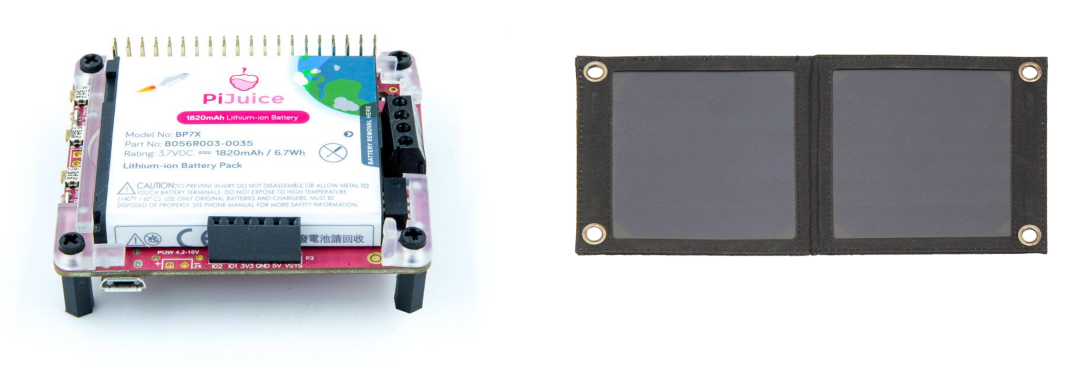
Regarding energy harvesting, several solutions are feasible, such as solar, eolic, and hydro. We decided to investigate the deployment of sunlight energy generation since solar panels are cheap, effective, and readily available on the market. Among the several solutions currently available, the Raspberry Pi ecosystem provides excellent solutions for managing self-powered systems through solar energy harvesting. Specifically, they enable to couple a small rechargeable battery, referred to as PiJuice Hat, perfectly fitting the multiple Raspberry Pi designs with small solar panels named PiJuice Solar. Figure 4 shows a Raspberry Pi self-powered by these two devices. Despite our choice, it is worth noticing that there are even cheaper alternatives for solar panels and rechargeable batteries. For instance, a general-purpose 6 W solar panel costs around 60 $ (https://www.sparkfun.com/products/13783) while the equivalent Raspberry Pi device is priced around 120 $ (https://uk.pi-supply.com/products/pijuice-solar). However, devices within the Raspberry Pi ecosystem can be seamlessly deployed without any hardware modification, simplifying the overall setup even when faced by not-specialized operators. For this reason, we stick to these devices, although, with minor efforts, the overall cost of the setup proposed could be significantly reduced.
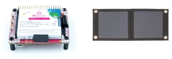
Figure 4.
(Left) Raspberry Pi with a PiJuice Hat battery on top of it, (Right) PiJuice Solar panel (6 Watt model). More details available at https://uk.pi-supply.com/products/pijuice-standard (accessed on 28 July 2021).
The PiJuice Hat is a small rechargeable battery fitting on the top of every Raspberry Pi device, including models 3B/3B+ and 4 considered in this paper. It is available with a different battery capacity of 1820 mAh, 2300 mAh, 5000 mAh, and 12,000 mAh, and includes a real-time clock. More details are available at this link: https://uk.pi-supply.com/products/pijuice-standard (accessed on 28 July 2021).
The PiJuice Solar is a cheap, lightweight, and water-resistant solar panel compatible with the PiJuice Hat. It is available in multiple variants providing 6, 12, 22, and 20 Watt when exposed to direct sunlight. More details are available at this link: https://uk.pi-supply.com/products/pijuice-standard (accessed on 28 July 2021).
6. Experimental Results
To assess the effectiveness of the setup, in this section, we illustrate experimental results on the application of the architectures on continuous surface flow monitoring that keep efficiency as a priority.
6.1. Evaluation Protocol
To identify the most efficient and effective solution among the platforms previously described, the following evaluation protocol has been put together: a USB camera is used to capture images at 1430 × 1080 resolution with each Raspberry Pi. The camera is an Aukey FHD 1080p Webcam PC-LM1E. The computing platform is remotely controlled via the WiFi network and a Bluetooth multimeter is used to log voltage and amperage consumption three times per second. The complete setup is described in Figure 5. To further minimize energy consumption, unused modules (HDMI and Bluetooth) have been turned off; the Ethernet port and USB hub are handled by the same device, thus they are both turned on only when the camera is framing the scene. The WiFi module can not be disabled during testing to monitor and control the device; however, it will be turned off at in situ deployment. Finally, it is worth noticing that, alternatively to a USB camera, a camera connected directly to the Raspberry Pi dedicated connector could also be used.

Figure 5.
Overview of the measurement setup. The Bluetooth digital multimeter allows three measurements per second.
As proposed in [3], to speed up computation and reduce energy requirements, we consider efficient computing paradigms and resources available for the Raspberry Pi-integrated ARM processors. Specifically, we run optimized versions of OTV that take advantage of ARM Single Instruction Multiple Data (SIMD) and the four-core CPUs (Multicore) capabilities available in all the Raspberry devices considered. Furthermore, we run the original algorithm on a single core of the CPU to serve as baseline. Concerning SIMD instructions, we exploit the NEON instruction set [13], while, for Multicore, we rely on the TBB framework [14]. The OpenCV library [15] (version 4.5 in our experiments) seamlessly allows for exploiting both computing facilities. As already mentioned, we do not use the computing resources available in the ARM GPU since, according to our experiments with Raspberry model 3B/3B+, they did not provide any evident advantage and are not even currently supported in model 4.
Regarding the parameters of the OTV algorithm, we use the same proposed in [3], and evaluate its performance at three resolutions: Full (1430 × 1080), Half (715 × 540), and Quarter (357 × 270). Specifically, we skip one out of two frames, tracking at most 15,000 FAST features. Moreover, concerning the Lukas–Kanade algorithm, we set a search area of radius 4, deploying three pyramidal levels. To evaluate the feasibility of running OTV on the embedded setups, we apply the algorithm on on a 20-s sequence acquired on the Brenta river at 25 Hz and previously studied in [1,3]. Furthermore, considerations on power consumption are drawn by using the USB camera to capture a 20-s video indoor.
6.2. OTV Algorithm: Outcome with Color and Monochrome Images
We test OTV accuracy in case of both monochrome and color images. Indeed, feeding OTV with monochrome images in place of color ones, as proposed initially in [1,3], proved to reduce processing time and power consumption. Figure 6 reports the outcome of OTV (Min velocity, Max velocity, Mean velocity, and its standard deviation) at Full (F), Half (H), and Quarter (Q) resolution. It can be noticed that, at the F and H resolutions, the outcome of OTV with monochrome images is always on par with the one obtained using color images. On the other hand, there is a significant gap at Q resolution regarding the Max velocity metric. A deeper investigation revealed that this problem might occur even with color images shrinking images excessively. In particular, tiny images fed to the pyramidal Lucas–Kanade algorithm may become so small that they lose the most meaningful information content to perform optical-flow estimation reliably. On the one hand, in general, the deeper the pyramid, the faster the execution time. On the other hand, too many pyramid levels may shrink images excessively at the deepest one. Therefore, a strategy to deal with this problem might consist of reducing the pyramid depth. For instance, setting a pyramidal level of 2 in the Tevere sequence fixes the problem highlighted. Nevertheless, at the Q resolution, this strategy might fail with other sequences such as that concerning the Secchia river. On the other hand, although a pyramidal level of 3 might be a good choice overall, tuning the pyramid depth at H resolution to be on par with results at F resolution might be helpful in some circumstances. According to this preliminary analysis, images are processed only at the F and H resolutions, setting a pyramidal level 3 in the Lucas–Kanade algorithm as proposed in [1,3] to evaluate energy requirements in the reminder.
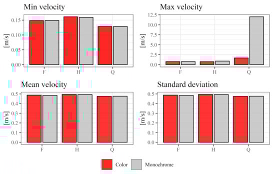
Figure 6.
Outcome of the OTV algorithm for color and monochrome video streams at full (F), half (H), and quarter (Q) resolutions.
6.3. OTV Algorithm: Power Consumption on Embedded Devices
Here, we evaluate the performance of the setup configurations previously outlined in terms of power consumption and execution time.
Figure 7 shows the execution time of the standalone OTV algorithm with the three computing platforms, for the two resolutions F and H, and with color and monochrome images. Not surprisingly, the Raspberry 4 is always significantly faster than the other two devices; on the other hand, the Raspberry Pi 3B is always the slowest one, although not far from model 3B+. We can also notice the same behavior when processing monochrome images but with a much shorter execution time, halved in most cases. Taking advantage of the four cores of the integrated CPU and the SIMD instruction set allows always for achieving the best performance enabling a notable speed-up compared to the baseline. In the optimal SIMD/Multicore configuration, processing a 20-s video stream takes a maximum of about 150 s (model 3B, full resolution colored images), or a minimum of time comparable to the processed video length (model 4, half resolution monochrome images). Interestingly, processing colored images with model 4 with the most efficient SIMD/Multicore configuration at both resolutions takes the same time needed for processing monochrome images with model 3B.
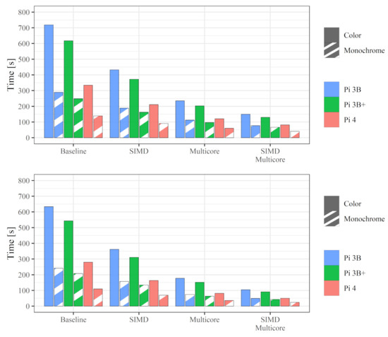
Figure 7.
OTV algorithm: execution time at (Top) full resolution and (Bottom) half resolution.
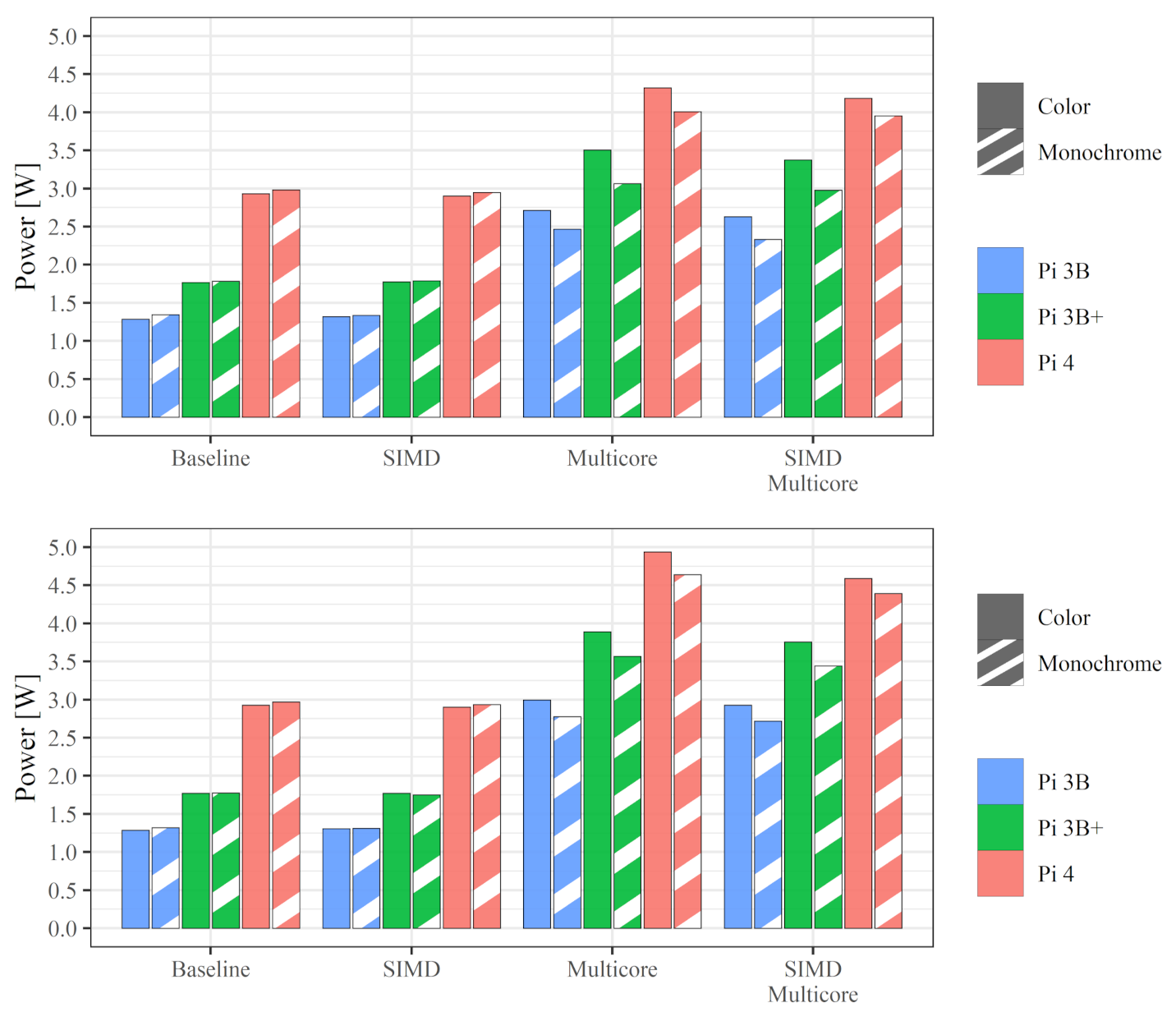
In Figure 8, it is shown that power consumption is not related to image resolution or SIMD; on the other hand, it conspicuously increases using all four CPU cores. Finally, from the power consumption point of view, using gray-scale images does not really matter even if it can be mildly beneficial using multicore. In the SIMD/Multicore configurations, the power required by model 3B is less than three watts, while, for model 4, it is higher than four watts in most cases.

Figure 8.
OTV algorithm: power consumption at (Top) full resolution and (Bottom) half resolution.
By combining execution time and power consumption, we can obtain the most relevant figure of merit: the energy required to carry out a single measurement with the OTV algorithm. Before doing so, we recall that energy E consumed by a device powered with voltage and draining current in the interval [, ] is the integral of power consumption over time:
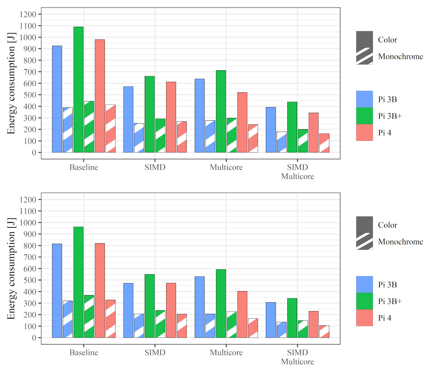
Observing Figure 9, it can be seen that processing gray-scale images at lower resolution is always beneficial in terms of energy consumption to perform a single measure. Specifically, monochrome images always allow for at least halving the energy drained by all devices. Image resolution also plays a beneficial yet less evident effect. An interesting outcome of the evaluation reported in Figure 9 concerns the fact that the Raspberry 3B+ turns out to be the most energy-consuming model, thus the worst choice when facing self-powered systems. Concerning the other two devices, although there is not an overall winner for each configuration, the device requiring less energy is always the Raspberry 4 configured to take advantage of SIMD and multicore capabilities.
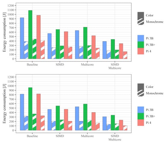
Figure 9.
OTV algorithm: energy drained during a single run at (Top) full resolution and (Bottom) half resolution.
6.4. Case Study: Periodic Surface Flow Monitoring
Once assessed the performance of the OTV algorithm, we address a case study motivated by practical considerations. Specifically, it is standard practice to perform surface flow measurement periodically, for instance, every 15 min. Consequently, in this case, it is possible to divide the whole 15-min cycle activity into the four phases outlined in Figure 10. Although the actual velocity estimation task takes place in the OTV phase, to obtain the energy drained in a 15-min cycle, three other phases (video acquisition, image extraction, and a low power idle state for the remaining time) must be taken into account. In our experiments, the video acquisition stage lasts 20 s and uses a USB camera, the next stage consists of extracting images from the video stored in RAM using the FFMPEG library. Besides OTV processing, the final phase (Idle) consists of a low-power state waiting for the following 15-min measurements. This latter phase (referred to as halt state according to the Raspberry terminology [16]), which lasts more than any other phase in our experiments, turns out to be critical since it impacts energy consumption significantly. Unfortunately, Raspberry PI 3B and 3B+ struggle compared to model 4 to save energy in the Idle phase; therefore, as detailed below, their efficacy is further decreased besides the considerations drawn in the previous section.

Figure 10.
The four phases composing a measurement cycle.
6.4.1. Overall Energy Consumption
Table 1 reports the energy drained by the three devices, at full and half resolution and with color and monochrome images, for each of the four phases outlined in Figure 10 during a 15-min measurement cycle. The table includes the overall energy, in bold, and in the rightmost column, the length of the idle time.

Table 1.
Energy consumed by the three devices, configured to take advantage of SIMD and Multicore processing capabilities, during each phase of a 15-min measurement cycle. Additionally, the rightmost column reports the seconds of idle time.
From the table, we can immediately notice that the figures of merit that emerged with the analysis focused on the single OTV phase also apply to a 15-min cycle measurement. The Raspberry Pi 3B+ is the least energy-efficient device, followed by model 3B, while the clear winner in all configurations is model 4, with a significant advantage compared to other devices. Specifically, compared to 3B and 3B+ in the same configuration, it always allows saving, respectively, more than 200 J and 350 J for each measurement cycle. For all devices, we can also notice that the energy consumed for monochrome image extraction from the 20-s video is halved compared to the color case, and once again, model 4 is the most efficient platform, even if by a small margin in this case. By looking at the idle time reported in the rightmost column of the table, we can notice, not surprisingly, that model 4 has the longest time in this phase. Its power management system is much more efficient than other devices, draining less than 1/3 currently. This fact, coupled with the energy figures that emerged in the OTV phase and the energy required for video extraction, always enables maximum energy efficiency deploying an out-of-the-box Raspberry Pi 4 system despite a slightly higher consumption for image acquisition. It is worth noting that a better energy handling of the idle phase would be possible with additional external circuitry for models 3B. However, it would add additional complexity/cost and hardly compensate for the default efficiency of model 4.
We recall that, when targeting the maximum energy efficiency with Raspberry Pi devices, it is crucial to disable via software commands USB ports when not strictly necessary since they drain a significant amount of energy. In our setup, the only phase requiring active USB ports is the acquisition phase, carried out with a color USB camera in our experiments, lasting for construction of the first 20 s of each measurement cycle.
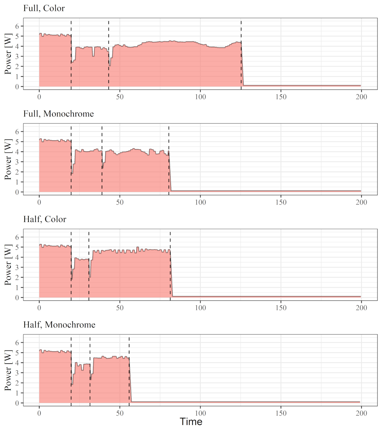
Figure 11, shows the instantaneous power consumption measured with a Raspberry 4 in the four examined configurations for the first 200 out of 900 s of a single measurement cycle. We can perceive how deploying monochrome images at half resolution is the optimal choice regarding energy efficiency.
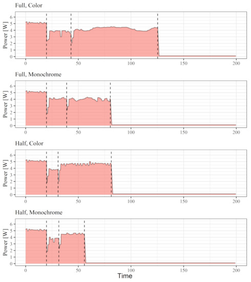
Figure 11.
Power consumption for the first 200 s of a 15-min measurement cycle with a Raspberry Pi 4 at Full and Half resolution with color and monochrome images. The area under each curve represents the energy consumed during each measurement cycle.
6.4.2. Analysis of Self-Powering Capability
Starting from the outcome of the previous section, we analyze now how the most energy-efficient device behaves when self-powered according to the setup outlined in the previous sections. Specifically, we consider the Raspberry Pi 4 in its optimal SIMD and Multicore configuration, processing color and monochrome images at full and half resolution. From Table 1, we can easily infer that our target device has the following average current drained, assuming a constant 5.1 input voltage, in the four following configurations:
- Raspberry Pi 4, Color images, Full resolution: 133.9 mA/h;
- Raspberry Pi 4, Monochrome images, Full resolution: 95.8 mA/h;
- Raspberry Pi 4, Color images, Half resolution: 101.2 mA/h;
- Raspberry Pi 4, Color Monochrome images, Half resolution: 74.7 mA/h.
To estimate battery life, we consider a subset of options available for the PiJuice Hat device. Specifically, we select batteries with a capacity of 5000 and 12,000 mA/h. By assuming fully charged batteries in ideal conditions, the following table reports the number of measurement cycles allowed.
For the successive considerations, we consider as a reference the city of Bologna in Italy. Its most extended daylight occurs on 21 June, and its length is 15 h, 33 min, and 1 s. Consequently, in such a scenario, it would be necessary to perform 63 measurement cycles per day. Looking at Table 2, assuming fully charged batteries, we can notice that such target is always fulfilled with the 12,000 mA/h battery, in any configuration. In contrast, with the smallest 5000 mA/h battery, the target number of cycles would be obtained only when processing monochrome images at half resolution. Interestingly, a fully charged 12,000 mA/h battery would allow for about two days of measurements. Nonetheless, even in this circumstance, battery charging is crucial, and we assume to carry it out with a PiJuice Solar panel, available in the 6, 12, 22, and 40 Watt options. According to the specifications available, the former can nominally provide up to 1000 mA/h when hit by appropriate sunlight, while the latter doubles this value. Therefore, the 6 Watt solar panel would allow for recharging the 5000 mA/h battery in 5 h and the 12,000 mA/h in 12 h. On the other hand, using a 12-Watt solar panel would allow for halving both recharging times. Although these are rough estimations, a setup made of a 12,000 mA/h battery coupled with a 12-Watt solar panel would probably be enough to handle even the worst-case scenario. For the city of Bologna, it could occur around 21 December, during the shortest daylight. In these circumstances, with a daylight length of 8 h 49 min e 43 s, a large battery and solar panel could suffice to enable the 36 measurements per day required even against extended sunlight shortages. Additionally, an oversized power supply system would also account for unavoidable inefficiency concerning the energy harvesting process that we have not considered in our estimation discussed so far, and in degradation of the battery and the solar panel.
Table 2.
Feasible measurement cycles with batteries of 5000 mA/h and 12,000 mA/h.
Finally, it is worth highlighting that, although our analysis focused on solar energy at hand and widely deployed when facing stream monitoring, other self-powering strategies could be seamlessly deployed or integrated with it.
7. Conclusions and Future Work
Automatic image-based surface flow monitoring is a well-known and influential methodology to tackle many real-world problems, as witnessed by recent research activities in this field. This paper starts from a state-of-the-art approach based on explicit feature matching to improve its performance and assess its energy requirements when targeting a self-powered monitoring system in situ. Specifically, we have considered the OTV algorithm, analyzing the relationship between energy and execution time on multiple low-cost computing platforms. Due to its significant diffusion, we considered representative target devices Raspberry Pi 3B, 3B+, and 4 to evaluate the possibility of designing affordable self-powered systems coupled with standard rechargeable batteries and solar panels. According to our analysis, with a fully-charged battery, the proposed algorithm coupled with standard off-the-shelf components allows in its most advantageous configuration up to 67 and 160 15-min measurements cycles, respectively, with 5000 and 12,000 mA/h battery capacity. Moreover, such devices can be easily recharged with solar panels of small size, making our proposal ready for deployment in countless target measurement sites, even in highly remote regions. These facts, coupled with the low budget required for the hardware components, enable a capillary diffusion of surface flow monitoring and deployment in developing countries.
Author Contributions
Conceptualization, S.M., A.C., F.T. (Fabio Tosi), F.T. (Flavia Tauro), S.G., E.T., F.A., and M.P.; methodology, A.C., A.-H.L., S.M., F.T. (Fabio Tosi), F.T. (Flavia Tauro), S.G., E.T., and F.A.; software, A.-H.L. and L.F.; validation, A.C., A.-H.L., L.F., S.M., F.A., and M.P.; formal analysis, S.M., A.C., F.T. (Flavia Tauro), S.G., E.T., F.A., and M.P.; investigation, A.C., A.-H.L., L.F., S.M., F.A., and M.P.; resources, A.C., A.-H.L., L.F., S.M., F.T. (Fabio Tosi), F.A., and M.P.; data curation, A.-H.L., A.C., and S.M.; writing—original draft preparation, A.-H.L., S.M., A.C., and L.F.; writing—review and editing, S.M., A.C., F.T. (Fabio Tosi), F.T. (Flavia Tauro), S.G., E.T., F.A., A.-H.L., L.F., and M.P. All authors have read and agreed to the published version of the manuscript.
Funding
F.T. (Flavia Tauro) acknowledges support by the Departments of Excellence-2018-Program (Dipartimenti di Eccellenza) of the Italian Ministry of Education, University and Research, DIBAF-Department of University of Tuscia, Project “Landscape 4.0—food, wellbeing, and environment”.
Conflicts of Interest
The authors declare no conflict of interest.
References
- Tauro, F.; Tosi, F.; Mattoccia, S.; Toth, E.; Piscopia, R.; Grimaldi, S. Optical Tracking Velocimetry (OTV): Leveraging Optical Flow and Trajectory-Based Filtering for Surface Streamflow Observations. Remote Sens. 2018, 10, 2010. [Google Scholar] [CrossRef] [Green Version]
- Raspberry Pi Foundation. Models. 2021. Available online: https://www.raspberrypi.org/products/ (accessed on 17 May 2021).
- Tosi, F.; Rocca, M.; Aleotti, F.; Poggi, M.; Mattoccia, S.; Tauro, F.; Toth, E.; Grimaldi, S. Enabling Image-Based Streamflow Monitoring at the Edge. Remote Sens. 2020, 12, 2047. [Google Scholar] [CrossRef]
- Pearce, S.; Ljubičić, R.; Peña-Haro, S.; Perks, M.; Tauro, F.; Pizarro, A.; Dal Sasso, S.F.; Strelnikova, D.; Grimaldi, S.; Maddock, I.; et al. An evaluation of image velocimetry techniques under low flow conditions and high seeding densities using unmanned aerial systems. Remote Sens. 2020, 12, 232. [Google Scholar] [CrossRef] [Green Version]
- Fujita, I.; Muste, M.; Kruger, A. Large-scale particle image velocimetry for flow analysis in hydraulic engineering applications. J. Hydraul. Res. 1997, 36, 397–414. [Google Scholar] [CrossRef]
- Brevis, W.; Niño, Y.; Jirka, G.H. Integrating cross-correlation and relaxation algorithms for particle tracking velocimetry. Exp. Fluids 2011, 50, 135–147. [Google Scholar] [CrossRef]
- Lucas, B.D.; Kanade, T. An Iterative Image Registration Technique with an Application to Stereo Vision. In Proceedings of the 7th International Joint Conference on Artificial Intelligence, IJCAI ’81, Vancouver, BC, Canada, 24–28 August 1981; pp. 674–679. [Google Scholar]
- Perks, M.T. KLT-IV v1. 0: Image velocimetry software for use with fixed and mobile platforms. Geosci. Model Dev. 2020, 13, 6111–6130. [Google Scholar] [CrossRef]
- Leitão, J.P.; Peña-Haro, S.; Lüthi, B.; Scheidegger, A.; de Vitry, M.M. Urban overland runoff velocity measurement with consumer-grade surveillance cameras and surface structure image velocimetry. J. Hydrol. 2018, 565, 791–804. [Google Scholar] [CrossRef]
- Winsemius, H.; Annor, F.; Hagenaars, R.; Luxemburg, W.; Van den Munckhoff, G.; Heeskens, P.; Dominic, J.; Waniha, P.; Mahamudu, Y.; Abdallah, H.; et al. OpenRiverCam, open-source operational discharge monitoring with low-cost cameras. In Proceedings of the EGU General Assembly, online, 19–30 April 2021. [Google Scholar]
- Noto, S.; Tauro, F.; Petroselli, A.; Apollonio, C.; Botter, G.; Grimaldi, S. Low cost stage-camera system for continuous water level monitoring in ephemeral streams. Hydrol. Earth Syst. Sci. Discuss. 2021. in review. [Google Scholar]
- Rosten, E.; Porter, R.B.; Drummond, T. Faster and Better: A Machine Learning Approach to Corner Detection. IEEE Trans. Pattern Anal. Mach. Intell. 2010, 32, 105–119. [Google Scholar] [CrossRef] [PubMed] [Green Version]
- Mitra, G.; Johnston, B.; Rendell, A.P.; McCreath, E.; Zhou, J. Use of SIMD Vector Operations to Accelerate Application Code Performance on Low-Powered ARM and Intel Platforms. In Proceedings of the 2013 IEEE 27th International Symposium on Parallel and Distributed Processing Workshops and PhD Forum, Cambridge, MA, USA, 20–24 May 2013; pp. 1107–1116. [Google Scholar] [CrossRef] [Green Version]
- Pheatt, C. Intel® Threading Building Blocks. J. Comput. Sci. Coll. 2008, 23, 298. [Google Scholar]
- Bradski, G. The OpenCV Library. Dr. Dobb’s J. Softw. Tools 2000. [Google Scholar]
- Raspberry Pi Foundation. Frequently Asked Questions. 2021. Available online: https://www.raspberrypi.org/documentation/faqs/#pi-power (accessed on 17 May 2021).


Publisher’s Note: MDPI stays neutral with regard to jurisdictional claims in published maps and institutional affiliations. |
© 2021 by the authors. Licensee MDPI, Basel, Switzerland. This article is an open access article distributed under the terms and conditions of the Creative Commons Attribution (CC BY) license (https://creativecommons.org/licenses/by/4.0/).