Article

Experimental Evaluation and Theoretical Optimization of an Indirect Solar Dryer with Forced Ventilation under Tropical Climate by an Inverse Artificial Neural Network

1
Col. Magisterial, Centro, Zona de la Cultura, Avenida Universidad S/N, Universidad Juárez Autónoma de Tabasco, Villahermosa C.P. 86040, Mexico
2
Facultad de Ingeniería, Campus V, Predio S/N Por Av. Humberto Lanz Cárdenas y Unidad Habitacional Ecológica Ambiental, Col. Ex Hacienda Kalá, Universidad Autónoma de Campeche, Campeche C.P. 24085, Mexico
3
Facultad de Ingeniería, Av. Industrias No Contaminantes S/N, Periférico Norte Apartado Postal 150 Cordemex, Universidad Autónoma de Yucatán, Merida C.P. 97310, Mexico
*
Authors to whom correspondence should be addressed.
Appl. Sci. 2021, 11(16), 7616; https://doi.org/10.3390/app11167616
Submission received: 16 July 2021 / Revised: 8 August 2021 / Accepted: 13 August 2021 / Published: 19 August 2021
(This article belongs to the Special Issue Renewable Energy in Agriculture Ⅱ)

Abstract

:
In this theoretical–experimental study is presented a hybridization strategy based on the application of an inverse artificial neural network model (ANNi) coupled with metaheuristic optimization algorithms to optimize the drying velocity (vd) of an active indirect solar dryer for plantain and taro (Colocasia antiquorum). In the experimental stage, both fruits were evaluated in periods from 9:00 a.m. to 5:00 p.m. under a humid tropical climate region, varying the voltage of the air extractor fan (at 6 V, 9 V, and 12 V) to control the fan velocity. The experimental results showed that the maximum drying velocities were reached at 9 V, achieving a drying velocity of 1.5, 0.9, and 0.55 g/min, with a total drying time of 465 min for the taro, and 1.46, 1.46, and 0.36 g/min, with a total drying time of 495 min, for the plantain. As a result of the drying curves, it was observed that the drying velocity is higher in taro than in plantain. Subsequently, an artificial neural network (ANN) architecture was trained using the database generated from the solar dryer’s experimental stage. Six environmental variables and one operational variable were considered as the model’s inputs, feeding the ANN to estimate the drying velocity (vd), obtaining a linear regression coefficient R = 0.9822 between the experimental and simulated data. A sensitivity analysis was performed to determine the impact of all the input variables. A hybrid strategy based on ANNi was developed and evaluated with three metaheuristic optimization algorithms; the best result was obtained by genetic algorithms (ANNi-GA) with an error percentage of 0.83% and an average computational time of 4.3 s. The scope of this optimization strategy was to obtain a theoretical result that allows predicting the behavior of the dryer and improving its performance for its practical application in future work through the implementation in development boards. Lastly, the optimization strategy presented is not limited to indirect solar dryers and opens a research window for evaluating other solar drying technologies.

1. Introduction

In Latin America, the Mexican agricultural industry is one of the most significant, establishing itself as the largest producer of vegetables in the region and occupying the second place in fruit exports worldwide. Agricultural activities play an essential role in the Mexican economy, with a contribution to gross domestic product (GDP) of more than 2% and an economic spillover from foreign direct investment (FDI), which in 2019 exceeded 50 million USD [1]. Among the country’s growing regions, the south-southeast zone (made up of the States of Tabasco, Chiapas, Campeche, and southern Veracruz) stands out due to its favorable climatic and hydrographic conditions, where 96% of the agricultural surface has rainwater irrigation. In this region, 50% of the entire country’s water runs off, and the prevailing tropical rainy climate allows for harvests practically all year round [2]. From 2011 to 2017, the south-southeast region sustained the highest agricultural growth, with an annual rise in the area, in real terms, of 35.7%, making this region very important for the national agricultural use [3]. However, the fact of having harvests almost all year round brings about an economic problem related to the placement and sale of the products. This process is subjected to the postharvest lifetimes of the crop since it can generate an excess of production, saturating the market, or generate economic losses for farmers, due to wastage. Therefore, alternatives are required to preserve seasonal food, helping the development of the rural economy.
One of the most attractive options for preserving fruits, vegetables, and herbs is drying and dehydration, which also provides other benefits such as lowering transport costs, increasing lifetime, and reducing crop waste [4]. Specifically, in regions with a tropical climate, solar dryers represent a feasible option for the development of such activity from an ecological approach, presenting lower capital and operating costs than conventional dryers [5]. In solar dryers, thermal energy from near-infrared wavelengths is harnessed to supply heat for the drying process and evaporate the required moisture content from the product. The effectiveness in the use of this technology depends on the radiation levels in the region. In the case of Mexico, the annual average daily irradiation on a horizontal surface is just over 4.4 kWh/m2·day. Specifically, in the south-southeast region, there is average daily irradiation of 5.5 kWh/m2·day due to its geographical location between the tropics of Cancer and Capricorn, the area where the most significant amount of solar radiation is captured in the world [6]. Therefore, the use of solar thermal technology in Mexico contributes significantly to the energy requirements for postharvest processing, with the adequate technical feasibility to be used as a technological improvement in agricultural areas of tropical climate regions (like the south-southeast region of Mexico).
Due to the agricultural biodiversity of this tropical region, in recent years, the practical potential of using solar thermal technology drying has been analyzed for various products with good commercial value for the south-southeast of Mexico [7]. M. Castillo Téllez et al. [8] developed an indirect tunnel type solar dryer for application in red chili. They evaluated the drying kinetics obtaining drying times of 2.75, 3.0, and 6.25 h, for temperatures of 55 °C, 65 °C, and 45 °C, respectively. They also evaluated the velocity ranges, between 0.7 and 2.6 m/s, reaching drying times and final moisture contents of 16 h, with 0.057 to 0.90 kgwater/kgdry mass, and 21 h, with 0.0611 to 0.109 kgwater/kgdry mass, respectively. López-Vidaña et al. [9] developed a passive solar dryer to operate as a mixed or indirect dryer for tomatoes in a tropical region; the drying efficiency was in a range between 5.47% and 4.48%, respectively. For their part, M. Castillo Téllez et al. [10] presented an experimental study for a Stevia leaf solar dryer. A comparative study was carried out between direct and indirect drying by natural and forced convection. The heat supplied by a solar water heating system was used through a water/air heat exchanger. Natural convection produced a drying time of 360 min, while forced convection produced a drying time between 550 min and 600 min. Without a shade mesh, these values were 250 min and 300 min, respectively. Likewise, it was shown that an indirect solar dryer can be controlled better than a direct one.
In the southeastern region of Mexico, there are two crops that have excellent economic viability due to their characteristics. One is the plantain, a product highly commercialized nationally and internationally, which can expand its economic potential if its postharvest processing is diversified and its production is maximized. Another crop is taro, a product with good nutritional properties, which has been underutilized; hence, its processing and use make it a market niche in the agro-industrial and food sector. To dry these products and to preserve their organoleptic properties, it is necessary to achieve drying temperatures that range between 60 °C and 75 °C. This makes it necessary to use low-temperature solar thermal technology capable of establishing limits to the UV radiation that may damage the samples. Thus, the best option for this purpose is an indirect solar dryer.
However, an indirect solar drying system comprises processes where different interconnected physical phenomena take place, such as energy interactions, mass exchanges, fluid movements, and heat flows, to mention a few. Therefore, it is a complex system whose analytical solution cannot be found, which implies finding numerical solutions [11]. On the other hand, during the drying process, it is crucial to monitor the different variables such as environmental conditions, temperatures inside the solar dryer, relative humidity, air velocity, incident solar radiation, the type of product to be dried, the initial moisture contents, and total mass of the product, since they are variables that affect the drying of the product [12]. Being able to determine the best operating conditions for the drying system implies cost reduction, higher thermal performance, reduced drying time, better use of solar energy, and better dehydration. Therefore, it is necessary to develop and implement tools that help solve the optimization problem [13].
Therefore, it is important to establish an optimization criterion that, as a function of the design variables, as well as the modeling, simulation, and validation stages, allows us to minimize an objective function to satisfy the system’s operating conditions and the physical restrictions of the system [14]. Furthermore, many control and optimization problems can be solved by simple regulators; however, some control loops require advanced optimization techniques, which allow us to achieve the desired optimal operating conditions and, at the same time, reduce the complexity of their solution [15,16]. A feasible solution is the use of artificial intelligence modeling techniques, combined with reverse-engineering strategies and heuristic optimization algorithms, such as artificial neural network (ANN), genetic algorithm (GA), particle swarm optimization (PSO), ant colony optimization (ACO), and deep learning [17,18].
Table 1 shows a qualitative analysis of the most recent studies for indirect solar dryers. As can be seen, these studies are categorized into different aspects, such as type of research, the modeling technique applied, the purpose of the research, variables of interest, type of ventilation, and type of analysis. Concerning the type of research, it was detected that few works simultaneously addressed the modeling and experimental approaches of indirect solar dryers [19,20]. In addition, it was identified that there is only one work that used artificial intelligence tools (diffuse modeling, Takagi–Sugeno type) for modeling the thermal phenomena that occur during the drying of the product [21]. With regard to the variables of interest, it was identified that the drying time was the most analyzed, followed by the drying efficiency, the pick-up efficiency, and the exergetic efficiency [22]; however, there are no reports of the drying velocity, despite it being an important parameter for the development of control strategies focused on improving production. Lastly, there are no works that analyzed the indirect solar dryers from the perspective of sensitivity analysis.
According to the literature review, there is no report of a study focused on optimizing and controlling a solar drying device; thus, a hybridization strategy with artificial intelligence and metaheuristic optimization techniques has not been used either. In the same sense, none of the reported works considered the drying velocity as a variable of interest to control. Furthermore, despite the knowledge of the variables that influence the operation of solar dryers, there are no studies that quantitatively describe the level of impact that environmental and operational variables have on the final product.
For this reason, in this work, an experimental study of an indirect solar dryer for tropical fruits of high economic potential was developed, using samples of plantain and taro, and a hybrid strategy was subsequently implemented based on an artificial intelligence model and a metaheuristic optimization algorithm. The optimization process considered the voltage of the air extractor inside the dryer as an operating parameter in order to improve the drying velocity. The objective was to theoretically establish the optimal control values for the drying operation from an inverse neural network solved with three metaheuristic optimization algorithms, in addition to determining the theoretical optimal drying speed for the process.

2. Materials and Methods

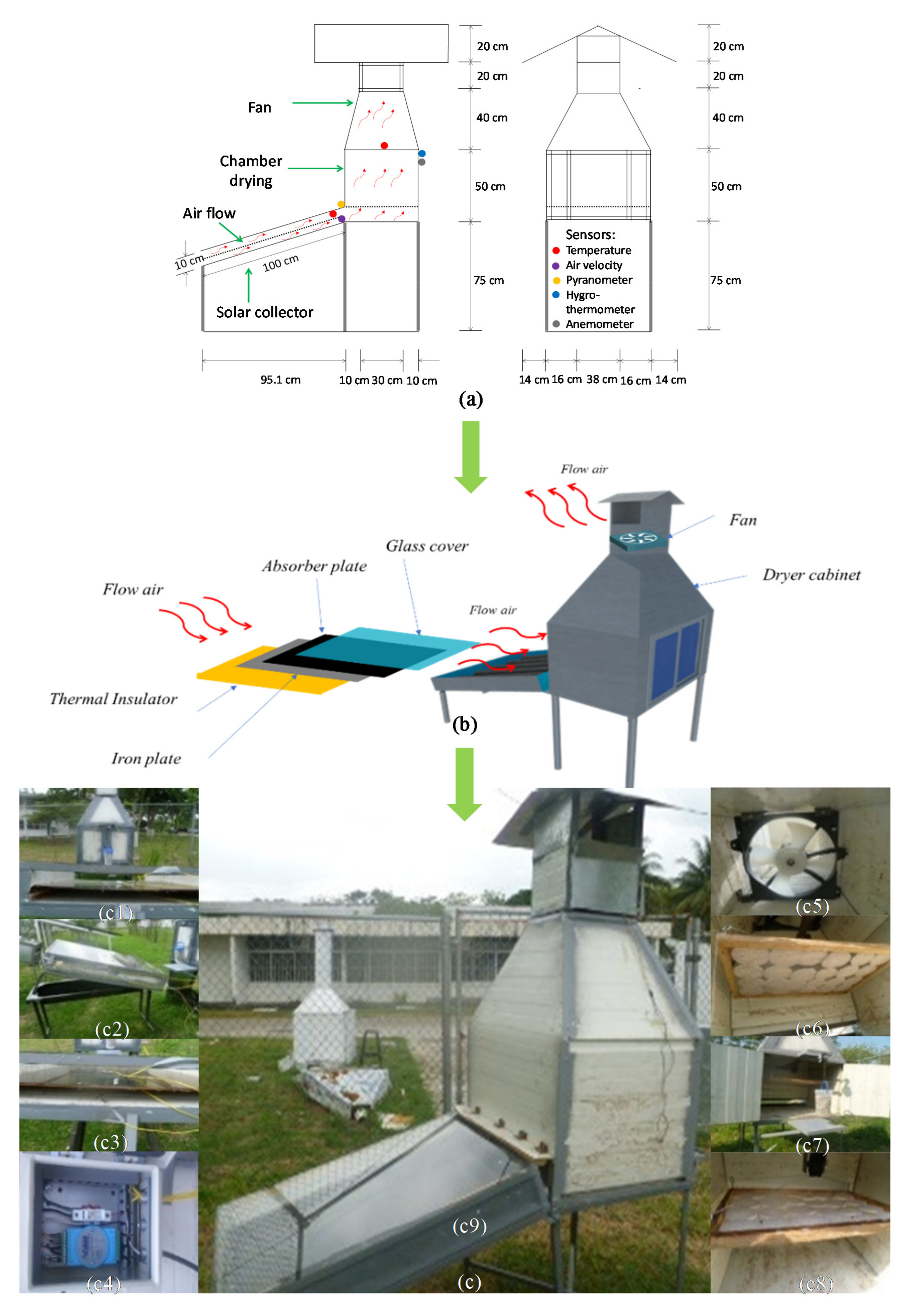
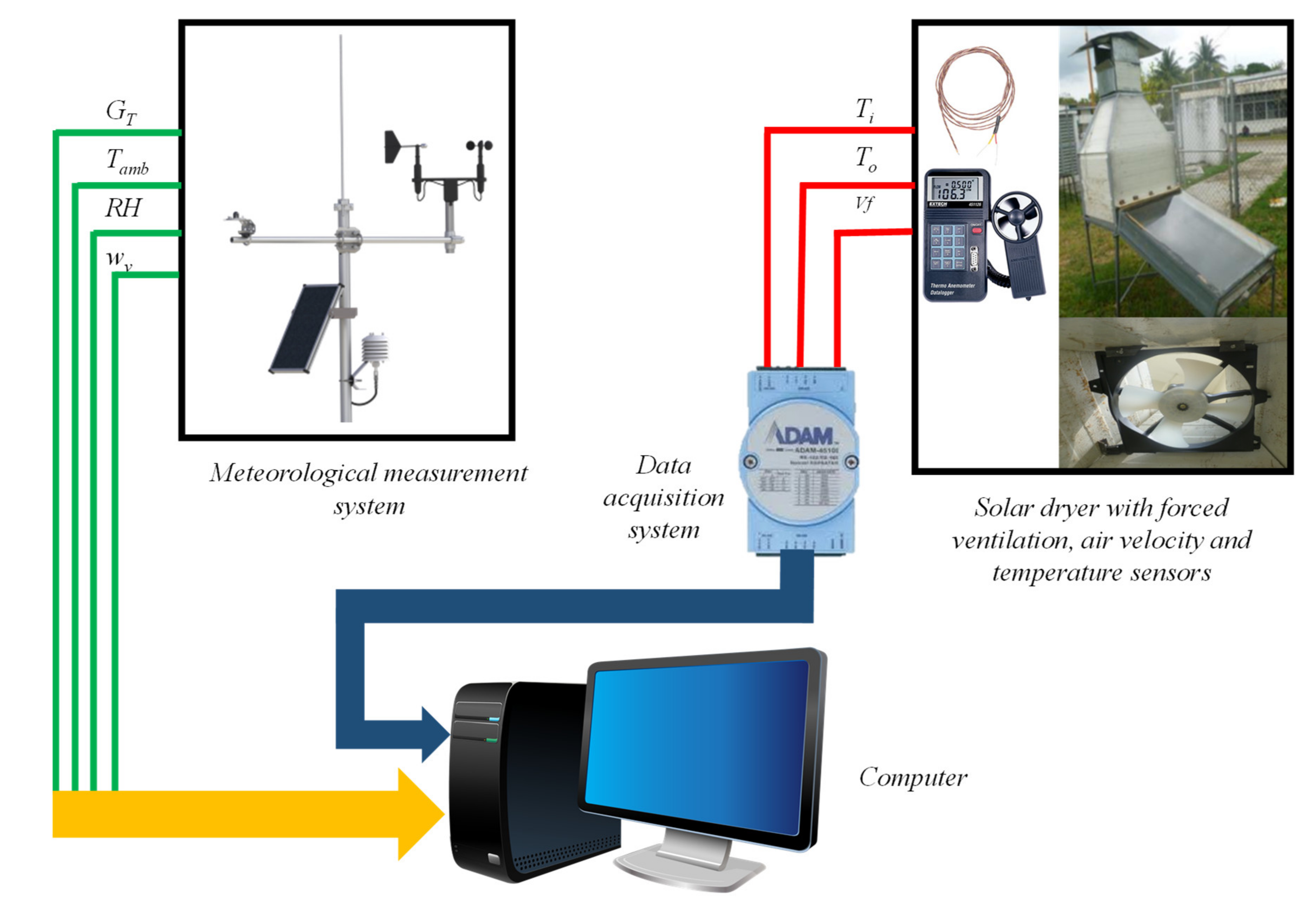
2.1. Description of the Experimental System

The experimental system used in the present study corresponds to a prototype of a solar dryer that operates by forced ventilation, designed mainly for drying plantain and taro. The prototype was evaluated in the Municipality of Cunduacán Tabasco, México, at the facilities of the Chontalpa Campus, Academic Division of Engineering and Architecture of the Juárez Autonomous University of Tabasco (18°4′24.27″ N latitude and 93°9′52.72″ W longitude).
Figure 1 shows the schematic diagram of the dryer used. It consists of a suspended absorber plate of stainless steel painted with a selective coating of nanostructured black nickel (α = 0.91; ϵ = 0.19), with a thickness of 4 mm and an area of 0.7 m2. The dimensions of the solar collector are 1.0 m × 0.7 m, with a fixed inclination angle of 18°. In order to minimize the heat losses to the environment, the bottom and sides of the collector were built with a central piece of thermal insulation using polyurethane panels coated with galvanized steel, with a thickness of 3.81 cm and a coefficient of thermal conductivity (k) of 0.018 W·m−1·K−1. The transparent cover is 3 mm thick clear glass (tc = 0.84, ϵc = 0.9 and αc = 0.06), to reduce heat loss at the entrance of solar radiation. The dimensions of the drying chamber are 0.7 × 0.5 × 0.8 m3, whereas its walls are also made with polyurethane panel covered with galvanized steel. The inside of the chamber has a metal guide to place the drying tray with dimensions of 0.6 × 0.45 m2, constructed with galvanized steel mesh. Above the drying chamber, there is a 1 m high chimney, with an opening in the outlet to allow the circulation of humid air outside the dryer. Lastly, to generate forced ventilation, a direct current (DC) fan with nominal values of 60 W, 12 V, 5.0 A, and 1800 rpm was installed on top of the chimney.
The solar dryer was instrumented to measure the environmental parameters that affect its performance and the operational parameters of interest. For the measurement of solar irradiance, an Amprobe Solar 100 pyranometer mounted on the solar dryer at an inclination of 18° was used. The temperature and relative humidity of the environment were sensed using an Extech RH101 Hygro-Thermometer hygrometer, while an Extech 451,126 fin anemometer was used for wind velocity. Concerning the operational parameters, the temperature inside the dryer was measured using type K thermocouples, distributed across the solar collector, the drying chamber, and the chimney. On the other hand, the air velocity inside the collector was measured using an Extech 451,126 anemometer, while the mass of the product to be dried was measured using a Torrey L-PCR 20 balance. Table 2 presents the technical information with the precision and operation ranges of these sensors. The sensors were connected to an ADAMS-4016 8-channel data acquisition card for the automated recording of information storage. The data were sent by network cable to a data logger, interconnected to a PC. The sampling period was 1 min with averages of 15 min. The selection of the sampling time at 15 min was carried out according to the design criteria for solar trackers, considering that the solar angle moves 1° every 15 min [12]. The schematic diagram of the experimental system is shown in Figure 2.
To measure the mass of evaporated water, a kilogram of fruit was sliced, placed in trays, and subsequently introduced to the solar dryer. The samples were left in the dryer for a period of 8 h. During this time, the set of all samples was weighed every 15 min and returned to the tray, identifying the evaporated water from the samples through weight loss. For practical terms, in each measurement, the mass of all the slices was quantified each measurement interval. In this period, the mass of water evaporated from the product was recorded to calculate the drying rate. This procedure was performed separately for both plantain and taro.
The experimental drying velocity was estimated as the ratio between the mass of evaporated water of the product and the drying time interval of the same. These values were obtained by measuring the loss mass of the fruit and the time elapsed between each sampling. This relationship is expressed by the following equation [34]:
v d = m w Δ t ,
where mw is the mass of evaporated water of the product (g), Δt is the drying time interval (min), and vd the drying velocity (g/min).

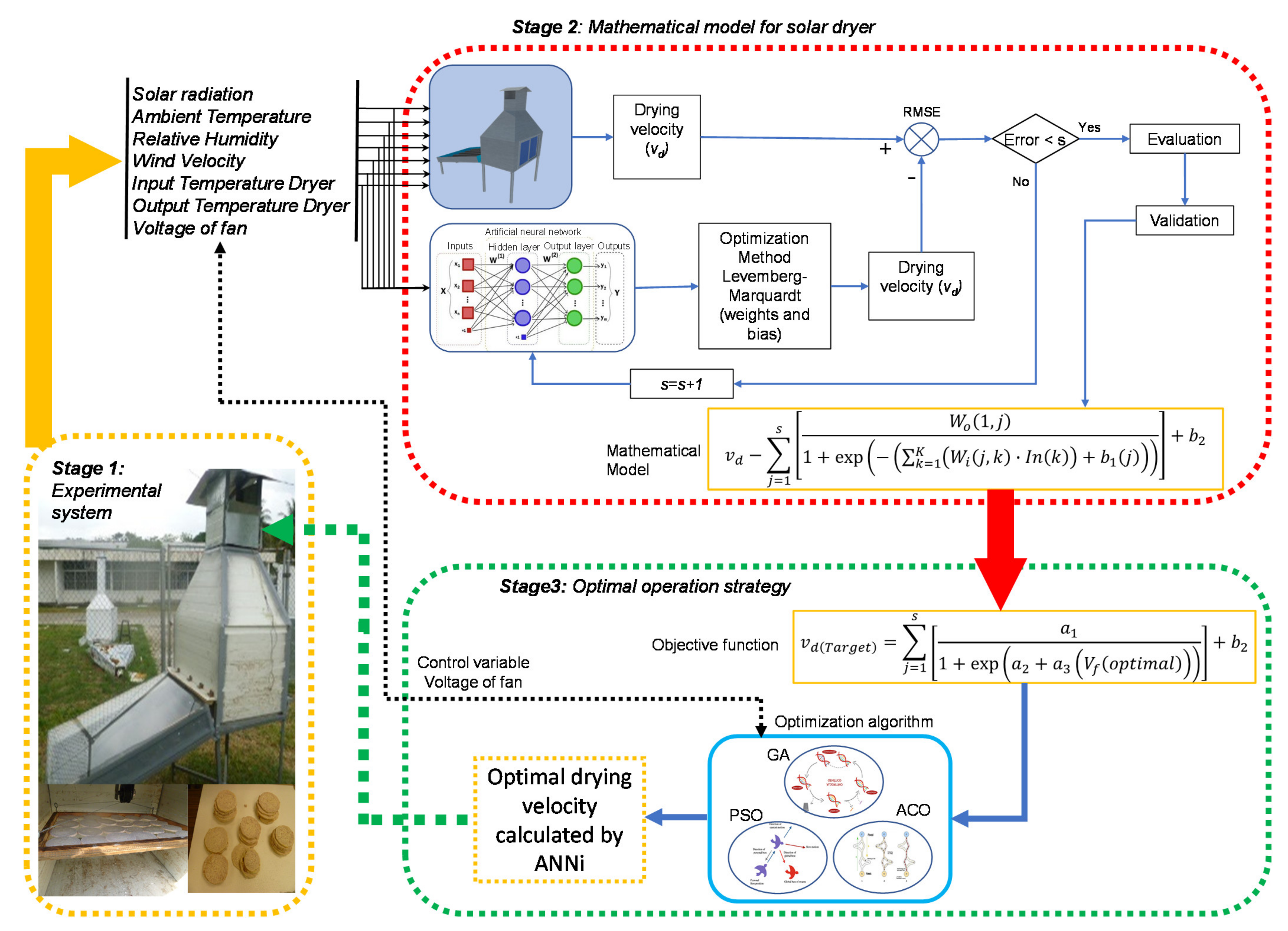
2.2. Computational Methodology

Figure 3 presents a diagram of the computational methodology used in the present work to specify the optimization process of the drying velocity for the proposed solar dryer. As can be seen, this is made up of three stages. The first stage consisted of creating an experimental database from the drying of plantain and taro by the photothermal device. This database was used in the second stage for the training and creation of a multivariate regression model based on ANN that correlated the environmental and operational measurements with the drying velocity of the samples. Once the optimal ANN model was obtained, it was used as an objective function to evaluate various metaheuristic optimization algorithms and determine which provided the best numerical results.

2.2.1. Experimental Database Construction

After implementing the experimental system, the measured data were collected and arranged in a spreadsheet according to the variables of interest. In total, a database made up of 3168 data was formed from eight experimental variables. For the development of the correlational model, the following variables were considered: solar radiation, ambient temperature, relative humidity, wind velocity, input temperature dryer, output temperature dryer, and fan voltage as the independent variables, and the velocity drying as the output variable. Table 3 summarizes the ranges of the variables considered in the present study.
Before training the ANN, the input variables were normalized because of the active functions’ nonlinearity and the operating range fluctuating between 0 and 1. These are special sigmoidal functions for activating the hidden layer. This normalization allows the surface of the error function to be reduced, making training more efficient, considering the initialization of the variables to zero. Each input variable was normalized using the following equation [35]:
u i , N = u i 1.1 × u m a x ,
where ui,N is the normalized variable, ui is the real value of the variable before normalization, and umax is the maximum value of the variable before normalization.

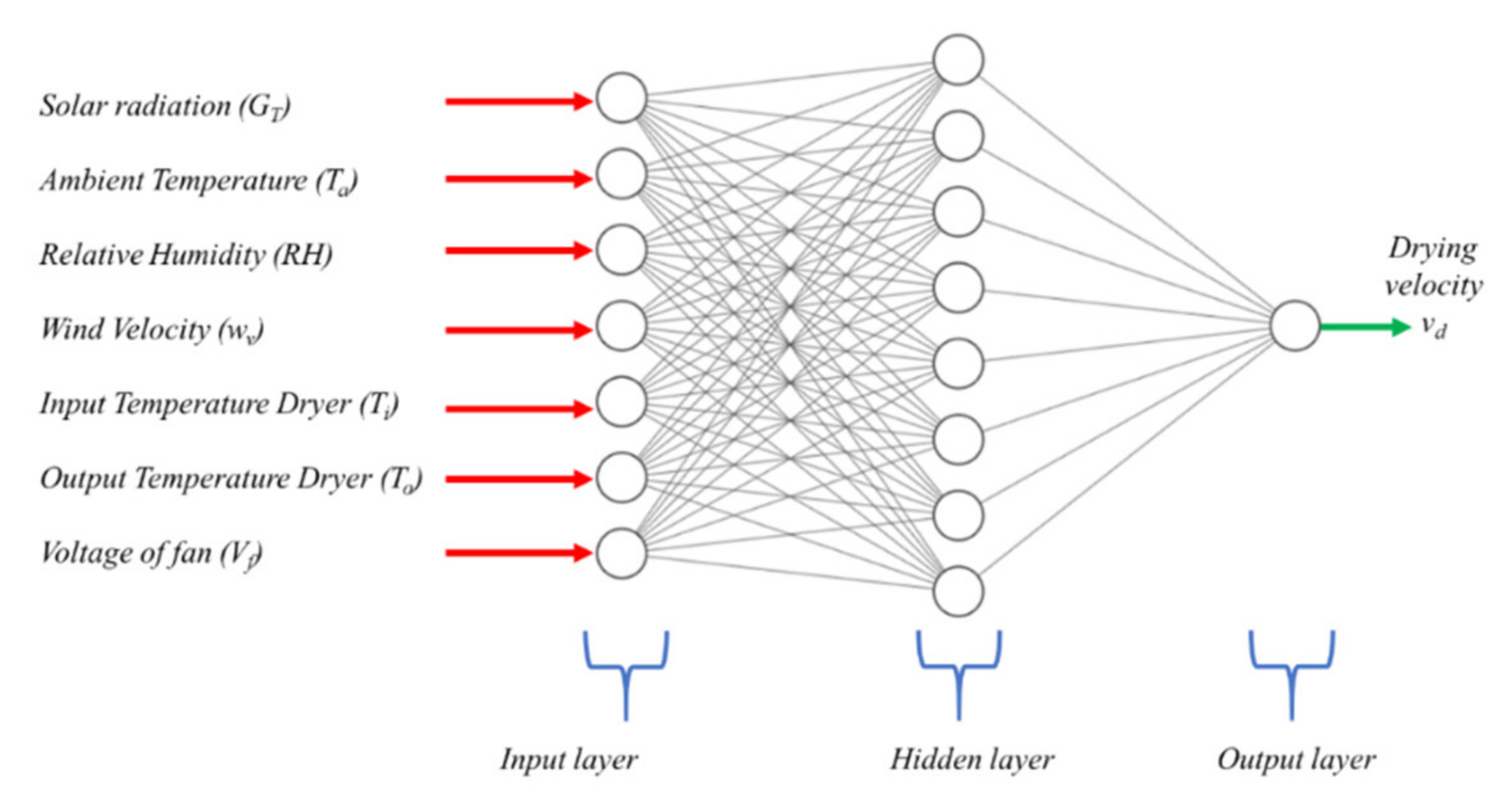
2.2.2. Artificial Neural Network Modeling

ANN was used as a computational tool [36] for the development of a mathematical model that correlates the environmental and operational parameters of the solar dryer to the drying velocity. The main reason for its choice is that it is one of the multivariate regression techniques with the greatest adaptability in complex thermal processes such as those exposed in this work [37]. In short, an ANN is a set of mathematical subfunctions called neurons, which are distributed in layers and interconnected with each other through constant values (weights). The ANN architecture used in this work consisted of an input layer, a single hidden layer, and an output layer. The numbers of neurons in the input and output layers were defined by the experimental variables in Table 3, while the hidden layer was made up of sigmoid neurons whose number was difficult to specify and required an iterative process for identification. In this work, two ANN architectures were evaluated with two different activation functions in the hidden layer, a hyperbolic tangent function and a logistic sigmoid, whose mathematical expressions with respect to their network architectures are presented in Equations (3) and (4).
v d ,   A N N = j = 1 s 2 × W o 1 , j 1 + exp 2 k = 1 K W i j , k · I n k + b 1 j + 1 + b 2 ,
v d ,   A N N = j = 1 s W o 1 , j 1 + exp k = 1 K W i j , k · I n k + b 1 j + b 2 ,
where Wi and Wo correspond to the connection weights of the neurons between the input–hidden layer and the hidden–output layer, respectively. The elements b1 and b2 represent factors of adjustments of the neural network associated with the neurons of the hidden layer and output layer, respectively. S and K represent the total number of neurons in the hidden layer and the input layer, respectively. Lastly, In represents the k-th input variable of the mathematical model.
For the development of the ANN model, the normalized input parameters contained in the database were used (Table 3). The data were randomly divided into subsets of training (80%), validation (10%), and testing (10%). By using a backpropagation algorithm to train the ANN through an iterative trial and error process, different numbers of neurons in the hidden layer were evaluated to find the optimal values of Wi, Wo, b1 and b2 for Equations (3) and (4) that minimized the error between the experimental data (xout,exp) and those estimated by the ANN (xout,sim). In this work, the backpropagation algorithm applied was Levenberg–Marquardt. This is a modification of the gradient descendent algorithm that performs numerical minimization processing to solve nonlinear least squares problems from an estimated initial parameter vector. The main advantage of using this algorithm is its fast convergence time, which is why it is widely used in ANN training [38].
To quantify the performance of the neuronal model, the following statistical criteria were used: root-mean-square error (RMSE), linear regression coefficient (R), coefficient of determination (R2), and mean absolute percentage error (MAPE), synthesized in Table 4.

2.2.3. Optimization Approach by Inverse ANN

In order to identify the fan voltages that guarantee optimal forced convection conditions to improve the operation of the solar system and achieve the maximum drying velocity, a computational strategy known as ANNi [39,40] was implemented, which is based on the algebraic reduction of Equations (3) and (4). This approach uses the coefficients of the weights and bias of the ANN obtained after their training (Wo, Wi, b1, and b2) and inverts the ANN to form the objective function defined by Equation (5).
y = v f b 2 + j = 1 s W o 1 , s ,
where y is the function of the experimental variable to be optimized (y = f(In(vd)). Equations (6) and (7) present the mathematical expressions for the case of ANN architectures with hyperbolic tangent and logistic sigmoid activation functions in the hidden layer neurons, respectively.
y = 2 s = 1 S W o 1 , s 1 + exp 2 k = 1 K X s + I n v d × W i j , k ,
y = s = 1 S W o 1 , s 1 + exp k = 1 K X k + I n v d × W i j , k ,
where X s is determined using Equation (8), from which K acquires all I n input values except for the one corresponding to v f ( I n v f = I n 7 ).
X s = k = 1 K 1 W i j , k × I n k + b 1 j .
Substituting Equations (4) and (5) into Equation (6), the objective functions for both network architectures can be obtained (hyperbolic tangent, Equation (9) and logistic sigmoid, Equation (10)).
y = 2 s = 1 S W o 1 , s 1 + exp 2 k = 1 K X s + I n v d × W i j , k b 2 + j = 1 s W o 1 , s .
y = s = 1 S W o 1 , s 1 + exp k = 1 K X k + I n v d × W i j , k b 2 + j = 1 s W o 1 , s .
For the solution of both objective functions, the evaluation of three metaheuristic optimization algorithms is proposed to determine the most efficient alternative dryer operation with the least computation time. The metaheuristic algorithms evaluated were genetic algorithm (GA), particle swarm optimization (PSO), and ant colony optimization (ACO). A detailed description of their operating principle is provided in Appendix A.

3. Results and Discussion

3.1. Experimental Evaluation of the Solar Dryer

The forced convection solar dryer prototype was experimentally evaluated during March, April, and May 2019, considering a drying schedule from 9:00 a.m. to 5:00 p.m. The experiments were carried out by applying different operating voltages to the fan (6, 9, and 12 V). Figure 4 and Figure 5 show the curves of moisture content on a dry basis and the velocity of drying referred to solar radiation for a test day, for taro and plantain, respectively.

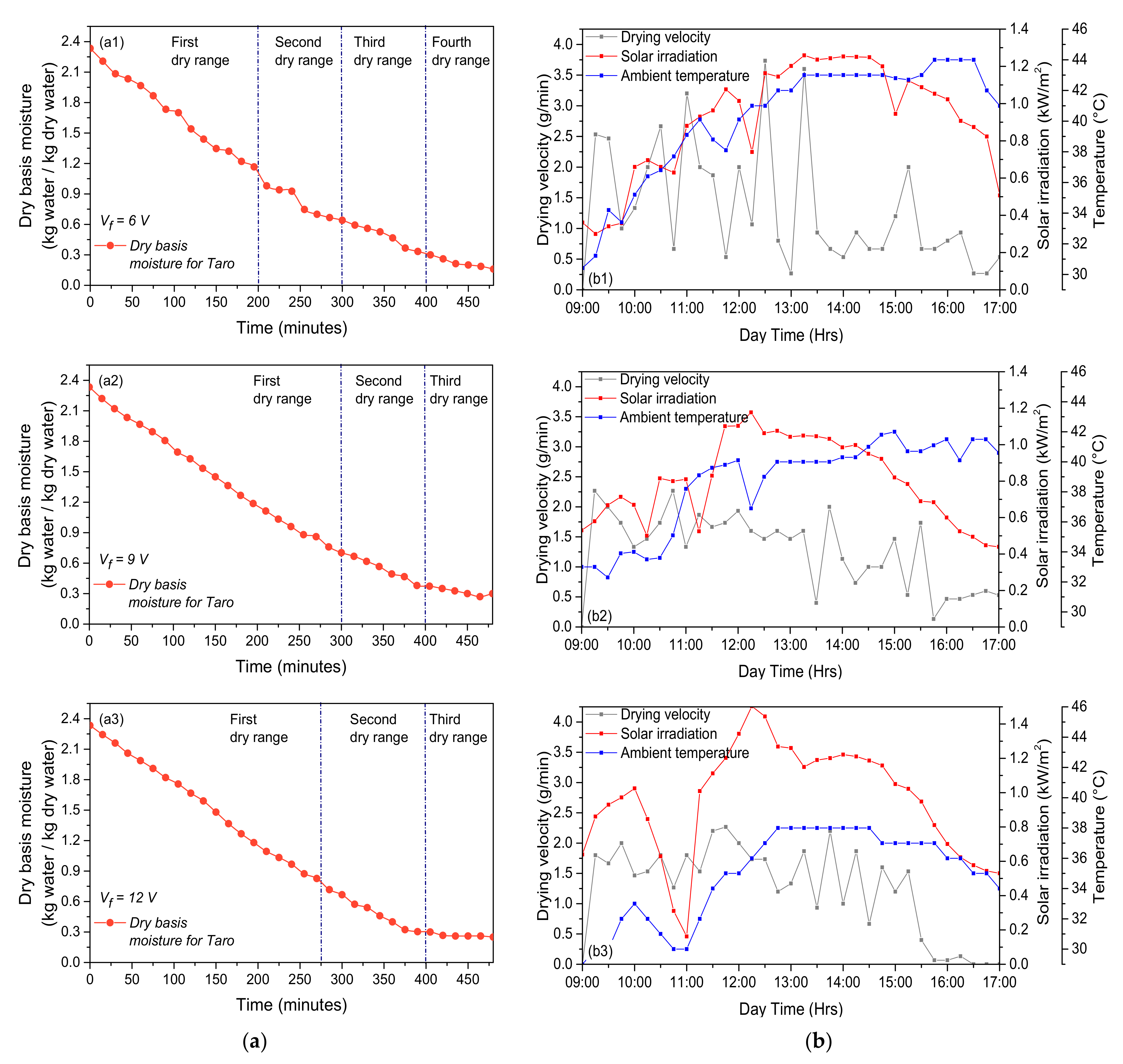
3.1.1. Taro (Colocasia esculenta)

Due to cloudiness, solar radiation had significant variations, which caused fluctuations in the air temperature at the entrance to the drying chamber. Three important aspects are combined in the phenomenology corresponding to the drying process: forced ventilation, the impossibility of maintaining constant the temperature of the air surrounding the samples, and the porosity of the taro. Due to its porosity, the critical moisture content in taro is high, which implies that the samples have a greater amount of water in the last drying stage (decreasing drying stage) and higher drying velocity than the plantain. The drying curves reflect the problem of migrating from the free moisture content zone and reaching the equilibrium moisture content, causing disturbances in the drying velocity curves. This is because the heat transfer rate is different from the mass transfer rate, which does not allow constant drying rates, and sudden changes occur since the concentration gradient decreases, sharply decelerating the mass transport and delaying the filling of water in the interstitial spaces of the taro by capillarity. However, the temperature gradient between the inlet of the solar collector and the outlet of the drying chamber could be maintained, and, despite the disturbances during the test, the evaporative drying conditions and behaviors were established.
In Figure 4, the drying curves for taro are observed, which were sectioned according to the deviations that occur in the drying velocity. The choice of the time ranges indicated in the subfigures was given by observing changes in the drying velocity curves, which showed different stages within the dryer. On the other hand, the derivative of the moisture content on a dry basis was considered because the drying speed was evaluated through the variations of the mass per unit of time, for each sampling period. In the case of the fan voltage at 6 V Figure 4(a1,b1), the drying time ranges were 0 to 200 min, 200 to 300 min, 300 to 450 min, and 450 to 525 min, with average drying velocities for each region of 1.8, 1.5, 0.9, and 0.3 g/min, respectively. These correspond to the changes in the dry basis moisture curve in the same ranges. According to the figures, despite the environmental conditions, the drying process stages were present, and a more stable drying velocity in the decreasing drying region was achieved, with a decrease of 33% compared to the previous region. In this case, the solar radiation and the ambient temperature conserved almost the same morphology during the entire test time, except for the period between 3:00 and 5:00 p.m. The temperature rose from 42 °C to 44 °C. This temperature rise helped sustain the drying process at the end of the curve.
In the case of the 9 V fan voltage (Figure 4(a2,b2)), the drying time ranges were 0 to 300 min, 300 to 400 min, and 405 to 465 min, with average drying velocities for each region of 1.5, 0.9, and 0.55 g/min respectively, corresponding to the changes in the dry basis moisture. The drying velocity curve in the first range presented a constant and prolonged rate of variation, while the drying velocity in the last time range decreased by 61% and stably maintained its decreasing velocity. According to the variations in solar radiation and ambient temperature, their behavior was at times similar in morphological terms, even more so from 3:30 to 5:00 p.m.; solar radiation decreased gradually, while the temperature remained oscillating between 40.7 °C and 41.5 °C, helping the drying process in its last stage.
In the case of the 12 V fan voltage (Figure 4(a3,b3)), the observed drying time ranges were from 0 to 270 min, from 270 to 405 min, and from 405 to 465 min, with average drying velocities for each region of 1.6, 1.17, and 0.53 g/min, respectively. These results correspond to the changes in the rate of variation of the dry basis moisture. Except for a disturbance at the beginning of drying, solar radiation remained with a favorable rate of change, maintaining its morphology concerning ambient temperature, including during the last hour and a half of the test where the decrease in solar radiation and ambient temperature agreed with the drastic decrease in drying speed. The average drying velocity decreased by 45.3% in the last time range, corresponding to the stability zone of the drying velocity.
From the conditions generated by the drying chamber and forced ventilation, and from the behavior of the drying curves, it was identified that the fastest drying velocities occurred when operating the fan at 9 V. It was observed that the average drying rates for the equilibrium moisture content drying region for the three voltage conditions were similar, with a value of 1.5 g/min, as well as for the first drying region, decreasing by 0.9 g/min. In contrast, in the second part of the decrease in drying, there was disparity, since the decrease percentages varied for each voltage at 33% for 6 V, 61% for 9 V, and 45.3% for 12 V, revealing the best drying conditions the 9 V experiment. From the above, we could perform a search to find the optimal voltage for drying, and this also allowed us to reduce the optimal response surface of the search.

3.1.2. Plantain

Similar to the case of taro, solar radiation had variations, albeit less significant in this case due to the presence of low cloudiness in the experiment period, improving the air temperature conditions at the entrance to the drying chamber. However, it was still not possible to keep a constant temperature of the air surrounding the fruit.
Contrary to taro, plantain porosity is low, also reducing the critical moisture content in the plantain. Due to this, plantain samples have less water in the last drying stage, and their drying velocity is lower than that of taro. Similar to the case of taro, there were disturbances, but they were decreased due to better conditions of solar radiation and a decrease in the porosity of the samples. The phenomenology was similar to that which occurs in taro. The temperature gradient for hot air circulation was still achieved, establishing the conditions and behaviors of drying by evaporation and improving the drying curves, as shown in Figure 5.
In the case of 6 V fan voltage, (Figure 5(a1,b1)), three drying time ranges were identified from 0 to 225 min, 225 to 350 min, and 350 to 465 min, with average drying velocities for each region of 1.27, 1.25, and 0.255 g/min respectively. This corresponded to the rate of variation of the dry basis moisture, which, at the beginning of drying, was observed to decrease, but not remain constant. The same behavior occurred for solar radiation, which only suffered from some disturbances at the beginning of the drying time. In Figure 5(a1), after 150 min, a behavior derived from a combination of effects was observed. On the one hand, there was a measurement error, which could be subject a change in the relative humidity of the environment. On the other hand, in the solar radiation curve, a sudden decrease of 0.735 kW/m2 occurred between 2:00 and 3:00 p.m., due to the presence of cloudiness. The temperature developed in a range between 32.3 °C and 44 °C, with a morphology similar to solar radiation, except for the sudden decrease in radiation, where the slow and delayed nature of the heating process was revealed, as there was no change in temperature until after the sampling period. In the last drying stage, a decrease of 20.4% in the drying velocity was achieved, 12.6 percentage points below the taro for the same supply voltage.
For the fan operating at 9 V (Figure 5(a2,b2)), two ranges of drying time were observed from 0 to 270 min and from 270 to 495 min, with average drying velocities of 1.46 and 0.36 g/min, respectively. The rate of variation of the dry base humidity ratio during the start of drying decreased and remained almost constant, thus covering a wide range of time (4.5 h). This was due to a reduction in disturbances of solar radiation, as well as the ambient temperature, reaching values between 38 °C and 28 °C, which also allowed a stabler and broader decreasing drying region of almost 3.75 h, with an average drying velocity of 0.36 g/min and a 25% reduction in drying velocity, 36 percentage points below the taro for the same supply voltage.
In the case of the fan at 12 V, (Figure 5(a3,b3)), three ranges of drying time were presented from 0 to 200 min, 200 to 345 min, and 345 to 435 min, with average drying velocities for each region of 1.95, 0.79, and 0.12 g/min, respectively. It was observed that disturbances only occurred in the solar radiation curve in the second region of the drying time, with a negative peak of 0.232 kW/m2 between 11:00 and 11:30 a.m.; with these exceptions, solar radiation and ambient temperature maintained their relative morphology, with a range between 27.9 °C and 36 °C, helping the drying process. On the other hand, in the last stage of a decrease in drying, the average drying velocity was 0.12 g/min, with a reduction in drying velocity of 15.4%, 29.9 percentage points below the taro for the same feed voltage.
The fan voltage with the highest detected drying velocities was 9 V, reaching maximum average drying velocities of 1.46 and 0.36 g/min for each drying region, with a total drying time of 495 min. It was observed that the average drying velocities for the initial drying region and the three voltage conditions were consistent, in a range from 1.27 to 1.952 g/min. In contrast, there were significant deviations for the final drying region (0.255, 0.36, and 0.12 g/min for 6 V, 9 V, and 12 V, respectively) with percentage decreases for each voltage of 20.4%, 25%, and 15.4%, respectively. Therefore, it was possible to perform a faster and narrower search for the optimal voltage for plantain drying.

3.2. Artificial Neural Network Model

A mathematical model based on ANN was developed to obtain a numerical expression that relates the environmental conditions of the experiment and the operating variables of the solar dryer. All the numerical calculations were executed through the MATLAB software and its ANN toolbox complement, due to the ease and flexibility of the platform for the application of artificial intelligence codes [38]. This model considers GT, Ta, RH, wv, Ti, To, and Vf as the input variables and the drying velocity (vd) as the output variable.
The ANN model was trained through a supervised learning process in which 80% of the data were used to train the model. This process was aimed at minimizing the error between the measured dry velocity and that generated by the model. In parallel, 10% of the data assigned to validation were used to avoid overtraining the model and guarantee its generalizability. Lastly, the remaining 10% of data were used to verify performance using unknown data. During this supervised learning process, the maximum number of iterations and the validation check (deviation index between the training and validation results) were considered as stopping criteria. Furthermore, in order to enable the general predictive capacity of the ANN, the k-validation approach suggested by Paneiro and Rafael [41] was conducted.
Table 5 presents the evaluation of the different network architectures (using the hyperbolic tangent and logistic sigmoid activation functions) to find the optimal ANN model. According to the analysis, for both cases, although the network architecture with 10 hidden neurons presented the best performance, the differences obtained with respect to the architecture with eight hidden neurons were minimal. Thus, to obtain a shorter computing time and better use regarding computational resources, the latter was chosen; the architecture of the artificial neural network can be observed in Figure 6.
Figure 7 shows the regression curves between the simulated (vd,sim) and experimental (vd,exp) data of vd, for the models with the hyperbolic tangent (Figure 7a) and logistic sigmoid (Figure 7b) transfer functions. As can be seen, the model based on hyperbolic tangent (vd,sim = 0.9865 vd,exp + 0.1000) was the one with the least dispersion of data and was more in line with the values measured experimentally. The above is supported by the statistical information in Table 5, where, for the model with eight neurons in the hidden layer and with the hyperbolic tangent transfer function, the statistical parameters were as follows: RMSE = 0.1912, R2 = 0.9647, R = 0.9822, and MAPE = 31.9%. For the same neural model, but with the logistic sigmoid transfer function in the hidden layer, we had the following parameters: RMSE = 0.2139, R2 = 0.9521, R = 0.9757, and MAPE = 25.4%. In relation to results with this same approach reported in the literature, Cervantes-Bobadilla, et al. [42] reported acceptable RMSE values of 0.4052 and 2.9178, while, in this work, the corresponding values were 0.1992 and 0.2139. Furthermore, Ajbar, et al. [40] performed modeling with a similar ANNi approach, obtaining R values of 0.9753 and 0.9678, which were considered acceptable to proceed with the optimization phase. Compared to this, this study presented better correlation values (R of 0.9822 and 0.9757). In the case of MAPE, high values were presented, although the model was adequately adjusted, as proven above and as shown by the regression curves (See Figure 7). This is due to the fact that the drying curves presented regions close to zero, due to the phenomenology of the drying process itself, where the drying rates were close to zero toward the end of each experiment. This fact is important because the MAPE divides the absolute error from the real data; hence, real values that are close to 0 can significantly increase the MAPE [43].
Thus, the mathematical function that describes the behavior of the solar drying process under study was given by Equation (3). Table 6 summarizes the weights and biases of the neuronal model for the hyperbolic tangent transfer function. The neural model used these parameters to reproduce the values of vd during the optimization process.

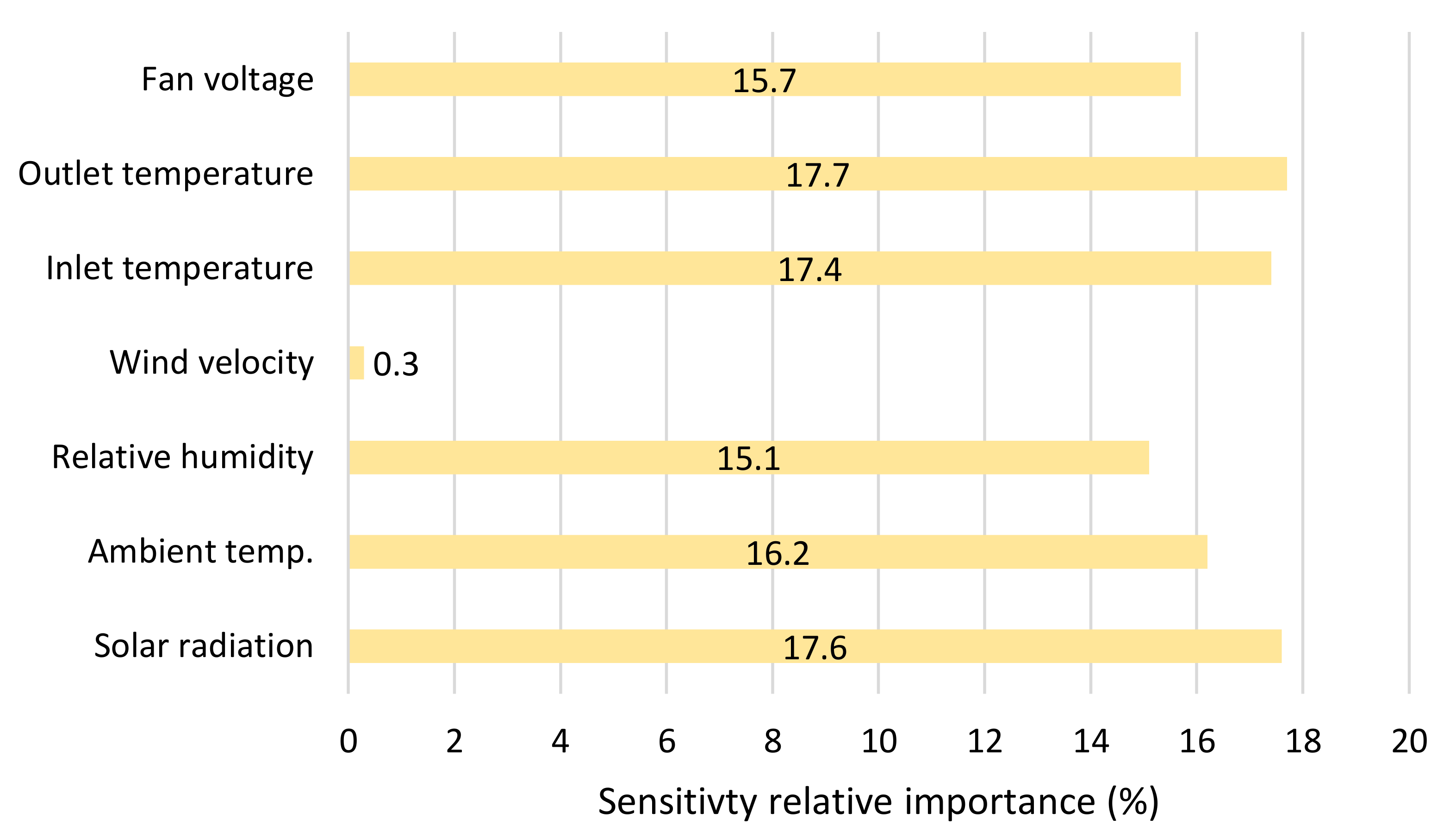
3.3. Garson Sensitivity Analysis

Once we obtained the artificial neural network model synthesizing the complex thermal processes inside the solar dryer in a single mathematical expression, a sensitivity analysis was performed using the Garson equation [44]. This determined the relative importance of the input variables on the drying velocity of the agricultural products evaluated. For this purpose, Garson’s equation takes into consideration the values of the weights (presented in Table 6), estimating the relative importance of each variable from the following mathematical expression:
I j = m = 1 N h W j m i h / k = 1 N i W k m i h · W m n h o k = 1 N i m = 1 N h W j m i h / k = 1 N i W k m i h · W m n h o ,
where Ij is the relative importance of the input variable j over the output variable, Ni and Nh are the numbers of input and hidden neurons, respectively, and W is the weight of the connection. The superscripts “i”, “h”, and “o” refer to the input, hidden, and output layers, respectively, and the subscripts “k”, “m”, and “n” refer to the input, hidden, and output neurons, respectively.
Figure 8 presents the results of the sensitivity analysis. It was determined that, except for the wind velocity, all the variables significantly impacted the drying velocity. In quantitative terms, the percentage of relevance was as follows: solar radiation (GT) (17.6%), ambient temperature (Ta) (16.2%), relative humidity (RH) (15.1%), wind velocity (wv) (0.3%), drying chamber inlet temperature (Ti) (17.4%), drying chamber outlet temperature (To) (17.7%), and fan voltage (Vf) (15.7%).
From these results, it can be seen that, due to it being a forced convection system, the effect of natural wind circulation was diminished. On the other hand, the wind velocity had a very low influence because there was not much variation in the database during the experiment (See Table 3), and the drying system was closed. The major influence regarding the wind velocity was represented by losses via convection on the surface, thus presenting a lower influence in the drying process. Likewise, the other parameters presented a similar significance level, differing by less than 2%. The fan voltage was shown to have an important impact, validating the application of control strategies as it is the only manipulable element.
Derived from the decoupling of wind velocity by forced ventilation, the other input variables were uniformly distributed, with an average contribution value of 16.61%. This means that they were strongly linked, due to the energetic interactions of the heat transport phenomena that occur in the drying process, such as the supply of heat by solar radiation to the solar collector. This heat is further injected into the air stream, raising its temperature to generate a gradient and provide the hot air flow, needed to remove any excess of water.

3.4. Optimal Operation Conditions

In this section, the inverse artificial neural network (ANNi) approach was implemented, considering as an objective function the ANN model developed (architecture 7–8–1; hyperbolic tangent activation function in the hidden layer). Based on the sensitivity analysis results and the discussion in Section 3.3, the ventilator’s operating voltage (Vf) was considered as the control variable. To establish a strategy in the theoretical operation that allows maximizing the drying velocity of both fruits (plantain and taro), the optimization of the objective function was expressed as follows in order to evaluate various operating scenarios considering the range used in the experimental process:
maximize :   min y = v d , s i m V f , subject   to :   V f j , m i n < V f j < V f j , m a x   where   j   =   6 to 12 .
To execute the optimization by ANNi, a Matlab script, aided by the Global Optimization Toolbox [45], was created in which the feasibility of the solution was evaluated using three different metaheuristic algorithms: genetic algorithm (GA), particle swarm optimization (PSO), and ant colony optimization (ACO) (described in detail in Appendix A). These algorithms were selected because they have shown successful results in the optimization of complex problems in diverse fields of research [46,47,48,49].
Using Equation (13), the error percentage ( ε ) was calculated to identify the ANN–metaheuristic optimization tuple that best approximates its calculations. In the same way, the computation time was recorded due to its importance during the possible execution of the optimization strategy in the operation of the fan voltage in real time.
ε = V f e x p V f o p t V f e x p × 100 %
Table 7 shows the results of implementing ANNi, considering a set of random samples of both plantain and taro that were not part of the training or validation model stages. The execution of the algorithms was carried out on a personal computer with an Intel i7 processor, eight cores, 16 threads, and 32 GB of RAM. Because the algorithms work based on stochastic methods, a total of 20 runs were performed to identify the average computation time to reach the solution. It is observed that, for this function, the smallest ε for each optimization strategy was as follows: 0.83% for ANNi-GA, with a computation time of 4.3 s; 1.11% for ANNi-PSO, with a computation time of 8.7 s; 3.00% for ANNi-ACO, with a computation time of 9.2 s. As can be seen, ANNi-PSO and ANNi-ACO presented the slowest calculation times of the three techniques evaluated; however, the percentage error for the optimal fan voltage for both algorithms was the highest. In comparison with ANNi-PSO and ANNi-ACO, ANNi-GA generated lower error rates, lower by 0.28 and 2.17 percentage points, respectively. Moreover, it presented better calculation times, with differences of 4.4 s and 4.9 s, respectively. The results of the table indicate that ANNi is an appropriate tool for application in indirect solar dryers, obtaining, for taro, error rates in the fan voltage lower than 3.33%, 5.56%, and 6.67% for ANNi- GA, ANNi-PSO, and ANNi- ACO, respectively, according to the experimental data. In the case of plantain, the errors were 5.33%, 4.58%, and 4.89% for ANNi-GA, ANNi-PSO, and ANNi-ACO respectively. By applying three different optimization algorithms to the ANNi, it was possible to obtain the input values associated with the solar dryer. As for the computational time, ANNi-GA applied to the plantain (5.3 s) required less time than for taro (5.5 s). When comparing the computation time with the different algorithms for the case of taro, a maximum difference of 4.4 s was obtained between ANNi-GA and ANNi-PSO, while 2.9 s was measured between ANNi-GA and ANNi-ACO, and 1.5 s was obtained between ANNi-PSO and ANNi-ACO. For plantain, the maximum computation time difference was between ANNi-GA and ANNi-ACO with 14.6 s, whereas the difference was 10.8 s between ANNi-PSO and ANNi-ACO and 3.8 s between ANNi-GA and ANNi-PSO. From the above, it was concluded that ANNi-GA is more likely to generate reduced computation time values.
From the optimization results, the small error margins imply that the fan voltage values can be reproduced to allow higher drying velocities and reduce drying times. In addition, the reduced computation time will make it possible to take full advantage of the sampling times of the drying process, as well as define better strategies for the use of control algorithms that allow fine adjustment, not only to reduce drying times. In terms of drying velocity, the results suggest establishing drying ramps to achieve drying with specific characteristics for other agricultural products, as shown by the development for taro and plantain.
In conclusion, the hybrid strategy of ANNi applied to metaheuristic optimization obtained good precision with an acceptable error range. The computation times are reasonable for a drying system since the control and optimization strategies can be implemented online for the applied sampling time, establishing an automatic working regime for low-temperature drying systems.

4. Conclusions

In this work, the design, instrumentation, experimental evaluation, and modeling of an indirect forced convection solar dryer with a chimney-type drying chamber were presented for its application in taro and plantain crops. A hybridization between artificial intelligence (artificial neural networks) and metaheuristic optimization techniques was established to obtain the operating conditions of the solar thermal system that maximize the drying velocity of the fruits. The system was evaluated under tropical climate conditions of the Mexican southeast by varying the fan voltage between 6 V and 12 V. The experimental results showed that, by applying a voltage of 9 V to the fan, the highest drying velocities were achieved for both fruits, which helped narrow down the search surface for the optimal answer.
From the point of view of both regional fruits, it was observed that, as the plantain has less porosity than the taro, it presented the best drying curves, taking less time to reach the critical moisture content. At the same time, the higher critical moisture content in taro allowed it to have a greater amount of water in its last drying stage, thus leading to higher drying velocities than in plantain.
An artificial neural network model was developed using the artificial intelligence application approach to estimate the drying velocity of both fruits, considering as independent variables the fan voltage, solar irradiance, ambient temperature, wind velocity, relative humidity, and the inlet and outlet temperatures of the solar dryer. The best network architecture consisted of eight hidden neurons, obtaining statistical values of RMSE of 0.1912, R2 of 0.9647, R of 0.9822, and MAPE of 31.9%, for a hyperbolic tangent transfer function in the hidden layer. Although the aim was not to replace existing theoretical models, the results indicate that the ANN is an efficient alternative to synthesize the thermal phenomena inside the solar dryer and estimate the drying velocity with reduced error margins. The first contribution of the ANN model was to perform a sensitivity analysis to determine the degree of influence of the input variables on the drying velocity of the evaluated fruits and its relationship with the phenomenology of the drying process. Except for the wind velocity, all the variables had a significant impact on the drying velocity, and the fan voltage could be determined as the control variable allowing us to achieve the optimal theoretical response.
The second theoretical contribution of the ANN model was its use as an objective function to optimize the drying velocity. The application of the ANNi method allowed finding the optimal voltage for a given drying velocity. The ANNi was evaluated with three different types of metaheuristic optimization algorithms, obtaining the following hybridization results: genetic algorithm (ANNi-GA) with an error percentage of 0.83% and a computation time of 4.3 s, followed by particle swarm particle optimization (ANNi-PSO) with an error of 1.11% and a computation time of 8.7 s, and ant colony optimization (ANNi-ACO) with an error of 3.00% and 9.2 s of computation time.

Author Contributions

Conceptualization, M.M.-B. and E.R.-M.; methodology, A.B. and O.M.T.; software, G.M.-P.; validation, M.M.-B. and V.C.-F.; formal analysis, L.R.-B.; investigation, E.R.-M.; writing—original draft preparation, M.M.-B. and O.M.T.; writing—review and editing, O.M.T., V.C.-F. and A.B.; visualization, G.P.-H. All authors read and agreed to the published version of the manuscript.

Funding

This research received no external funding.

Institutional Review Board Statement

Not applicable.

Informed Consent Statement

Not applicable.

Data Availability Statement

The data used to support the findings of this study are available from the corresponding author upon request.

Acknowledgments

The first author thanks the Postgraduate Program in Engineering Sciences of the Autonomous University Juárez de Tabasco for the support received during doctoral training.

Conflicts of Interest

The authors declare no conflict of interest.

Appendix A

Algorithm for genetic algorithm (GA) optimization.
Table A1. Pseudocode and parameters used to develop the genetic algorithm [50].
LineType AlgorithmSimulation Parameters
Genetic AlgorithmParameterValue
1Initial population Pobn = 100Generations (Genn)250
2for g = 1 to Genn = 250 doPopulation (Pobn)100
3for i = 1 to Pobn doMutationUniform
4Individual fitness i = {Tout-simTout-exp}CrossoverUniform
5end forSelectionrandom
6move the best fitness to population g + 1
7for i = 2 to Pobn do
8Selection of two individuals
9Apply crossover to create two new individuals
10Apply mutation to the remaining population
11end for
12move new individual, mutate and crossed to population (g + 1)
13end for
Algorithm for particle swarm optimization (PSO).
Table A2. Pseudocode and parameters used to develop particle swarm optimization [51].
LineType AlgorithmSimulation Parameters
Particle SwarmParameterValue
1Initialization for particle 1 to N
Initialize the position xi (0) ∀ i ∈ 1: N
Initialize particle best position to initial position pi (0) = xi (0)
Calculate the fitness of each particle and, if ƒ(Xj(0)) ≥ ƒ(Xi(0)) ∀ ij, initialize the global best as g = xj(0)
Steps (ns)100
2while stopping criteria is not reachedParticles (N)250
3Update velocity for particle using the equation:
vi (t + 1) = vi (t) + ci (pi − xi(t)) R1 + c2 (g − x(t)) R2
Cognitive parameter (c1)1
4Update the particle position using the equation:
xi (t + 1) = xi(t) + vi (t + 1)
Social parameter (c2)2
5Evaluate fitness of the particle ƒ (Xi (t + 1))Minima Inertia weight (w1)0.9
6if ƒ (Xi (t + 1)) ≥ ƒ(pi), update particular best: pi = xi (t + 1) Maxima Inertia weight (w2)0.2
7if ƒ (Xi (t + 1)) ≥ ƒ(gi), update global best: gi = xi (t + 1)
8end. The best solution is presented at the end of the iterative process by g
Algorithm for ant colony optimization (ACO).
Table A3. Pseudocode used to develop ant colony optimization [52].
LineType Algorithm
Ant Colony
1Input: Probsize, Populationsize, n, α, γ, θ, g0
2Output: O
3O ← Solution (Probsize);
4OcostCostCalculation (Ph)
5Init ← 1.0/(Probsize X Ocost);
6Pheromone ← Initialize (init);
7while Stop () do
8for x = 1 to n do
9Pi ← Solution (Pheromone, Probsize, γ, g0);
10Pxcost ← CostCalculation (Px);
11if Pxcost ≤ Ocost then
12OcostPxcost
13OPx;
14end
15LocalDecay (Pheromone, Px, Pxcost);
16end
17GlobaDecay (Pheromone, Pbest, Ocost, α);
18end
19return O;

References

  1. Centro de Estudios para el Desarrollo Rural Sustentable y la Soberanía Alimentaria. Situación del Sector Agropecuario en México. Available online: http://www.cedrssa.gob.mx/post_situacinin_del_-n-sector_agropecuario-n-_en_mn-xico.htm (accessed on 1 June 2021).
  2. Consejo Nacional Agropecuario. Zona Sur-Sureste, Potencial Agrícola. Available online: https://www.20minutos.com.mx/noticia/459003/0/zona-sur-sureste-region-con-tremendo-potencial-agricola/ (accessed on 1 June 2021).
  3. Financiera Nacional de Desarrollo Agropecuario, Rural, Forestal y Pesquero. Análisis del Centro de Investigación Económica y Presupuestaria. Available online: https://www.eleconomista.com.mx/estados/Sur-sureste-con-el-mayor-crecimiento-agropecuario-20180216-0019.html (accessed on 1 June 2021).
  4. Calín-Sánchez, Á.; Lipan, L.; Cano-Lamadrid, M.; Kharaghani, A.; Masztalerz, K.; Carbonell-Barrachina, Á.A.; Figiel, A. Comparison of Traditional and Novel Drying Techniques and Its Effect on Quality of Fruits, Vegetables and Aromatic Herbs. Foods 2020, 9, 1261. [Google Scholar] [CrossRef] [PubMed]
  5. Mohana, Y.; Mohanapriya, R.; Anukiruthika, T.; Yoha, K.S.; Moses, J.A.; Anandharamakrishnan, C. Solar dryers for food applications: Concepts, designs, and recent advances. Sol. Energy 2020, 208, 321–344. [Google Scholar] [CrossRef]
  6. Rosas-Flores, J.A.; Rosas-Flores, D.; Zayas, J.L.F. Potential energy saving in urban and rural households of Mexico by use of solar water heaters, using geographical information system. Renew. Sustain. Energy Rev. 2016, 53, 243–252. [Google Scholar] [CrossRef]
  7. Cortés-Rodríguez, E.; Pilatowsky-Figueroa, I.; Ruiz-Mercado, C.A. Feasibility Analysis of Drying Process Habanero Chili Using a Hybrid-Solar-Fluidized Bed Dryer in Yucatán, México. J. Energy Power Eng. 2013, 7, 1898–1908. [Google Scholar]
  8. Castillo-Téllez, M.; Pilatowsky-Figueroa, I.; López-Vidaña, E.C.; Sarracino-Martínez, O.; Hernández-Galvez, G. Dehydration of the red chilli (Capsicum annuum L., costeño) using an indirect-type forced convection solar dryer. Appl. Therm. Eng. 2017, 114, 1137–1144. [Google Scholar] [CrossRef]
  9. López-Vidaña, E.C.; Cesar-Munguía, A.L.; García-Valladares, O.; Pilatowsky-Figueroa, I.; Brito-Orosco, R. Thermal performance of a passive, mixed-type solar dryer for tomato slices (Solanum lycopersicum). Renew. Energy 2020, 147, 845–855. [Google Scholar]
  10. Castillo-Téllez, M.; Pilatowsky-Figueroa, I.; Castillo-Téllez, B.; López-Vidaña, E.C.; López-Ortiz, A. Solar drying of Stevia (Rebaudiana Bertoni) leaves using direct and indirect technologies. Sol. Energy 2017, 159, 898–907. [Google Scholar] [CrossRef]
  11. Lamidi, R.O.; Jiang, L.; Pathare, P.B.; Wang, Y.D.; Roskilly, A.P. Recent advances in sustainable drying of agricultural produce: A review. Appl. Energy 2019, 233–234, 367–385. [Google Scholar] [CrossRef] [Green Version]
  12. Duffie, J.A.; Beckman, W.A.; Blair, N. Solar Engineering of Thermal Processes, Photovoltaics and Wind, 5th ed.; Wiley: Hoboken, NJ, USA, 2020; pp. 650–664. [Google Scholar]
  13. Prakash, O.; Kumar, A. Solar Drying Systems; CRC Press: Boca Raton, FL, USA, 2020; pp. 1–28. [Google Scholar]
  14. Jaluria, Y. Design and Optimization of Thermal Systems, 3rd ed.; CRC Press: Boca Raton, FL, USA, 2020; pp. 339–372. [Google Scholar]
  15. Sendra-Arranz, R.; Gutiérrez, A. A long short-term memory artificial neural network to predict daily HVAC consumption in buildings. Energy Build. 2020, 216, 109952. [Google Scholar] [CrossRef]
  16. Tiumentsev, Y.V.; Egorchev, M. Neural Network Modeling and Identification of Dynamical Systems; Elsevier: Amsterdam, The Netherlands, 2019; pp. 93–128. [Google Scholar]
  17. Sarker, R.A.; Newton, C.S. Optimization Modelling: A Practical Approach; CRC Press: Boca Raton, FL, USA, 2008; pp. 233–236. [Google Scholar]
  18. Hernández, J.A.; Colorado, D.; Cortés-Aburto, O.; El Hamzaoui, Y.; Velazquez, V.; Alonso, B. Inverse neural network for optimal performance in polygeneration systems. Appl. Therm. Eng. 2013, 50, 1399–1406. [Google Scholar] [CrossRef]
  19. Blanco-Cano, L.; Soria-Verdugo, A.; Garcia-Gutierrez, L.M.; Ruiz-Rivas, U. Modeling the thin layer drying process of Granny Smith apples: Application in an indirect solar dryer. Appl. Therm. Eng. 2016, 108, 1086–1094. [Google Scholar] [CrossRef]
  20. Sekyere, C.; Forson, F.; Adam, F. Experimental investigation of the drying characteristics of a mixed mode natural convection solar crop dryer with back up heater. Renew. Energy 2016, 92, 532–542. [Google Scholar] [CrossRef]
  21. Zoukit, A.; Ferouali, H.E.; Salhi, I.; Doubabi, S.; Abdenouri, N. Takagi Sugeno fuzzy modeling applied to an indirect solar dryer operated in both natural and forced convection. Renew. Energy 2019, 133, 849–860. [Google Scholar] [CrossRef]
  22. Fudholi, A.; Sopian, K.; Alghoul, M.A.; Ruslan, M.H.; Othman, M.Y. Performances and improvement potential of solar drying system for palm oil fronds. Renew. Energy 2015, 78, 561–565. [Google Scholar] [CrossRef]
  23. Jain, D.; Tewari, P. Performance of indirect through pass natural convective solar crop dryer with phase change thermal energy storage. Renew. Energy 2015, 80, 244–250. [Google Scholar] [CrossRef]
  24. Misha, S.; Mat, S.; Ruslan, M.H.; Salleh, E.; Sopian, K. Performance of a solar assisted solid desiccant dryer for kenaf core fiber drying under low solar radiation. Sol. Energy 2015, 112, 194–204. [Google Scholar] [CrossRef]
  25. Ramos, I.N.; Brandão, T.R.S.; Silva, C.L.M. Simulation of solar drying of grapes using an integrated heat and mass transfer model. Renew. Energy 2015, 81, 896–902. [Google Scholar] [CrossRef]
  26. Essalhi, H.; Tadili, R.; Bargach, M.N. Conception of a Solar Air Collector for an Indirect Solar Dryer. Pear Drying Test. Energy Procedia 2017, 141, 29–33. [Google Scholar] [CrossRef]
  27. Lingayat, A.B.; Chandramohan, V.P.; Raju, V.R.K.; Meda, V. A review on indirect type solar dryers for agricultural crops—Dryer setup, its performance, energy storage and important highlights. Appl. Energy 2020, 258, 114005. [Google Scholar] [CrossRef]
  28. Atalay, H.; Çoban, M.T.; Kıncay, O. Modeling of the drying process of apple slices: Application with a solar dryer and the thermal energy storage system. Energy 2017, 134, 382–391. [Google Scholar] [CrossRef]
  29. Chandrasekar, M.; Senthilkumar, T.; Kumaragurubaran, B.; Fernandes, J.P. Experimental investigation on a solar dryer integrated with condenser unit of split air conditioner (A/C) for enhancing drying rate. Renew. Energy 2018, 122, 375–381. [Google Scholar] [CrossRef]
  30. Simo-Tagne, M.; Ndukwu, M.C.; Zoulalian, A.; Bennamoun, L.; Kifani-Sahban, F.; Rogaume, Y. Numerical analysis and validation of a natural convection mix-mode solar dryer for drying red chilli under variable conditions. Renew. Energy 2020, 151, 659–673. [Google Scholar] [CrossRef]
  31. Ekka, J.P.; Bala, K.; Muthukumar, P.; Kanaujiya, D.K. Performance analysis of a forced convection mixed mode horizontal solar cabinet dryer for drying of black ginger (Kaempferia parviflora) using two successive air mass flow rates. Renew. Energy 2020, 152, 55–66. [Google Scholar] [CrossRef]
  32. Lingayat, A.; Chandramohan, V.P.; Raju, V.R.K.; Kumar, A. Development of indirect type solar dryer and experiments for estimation of drying parameters of apple and watermelon. Therm. Sci. Eng. Prog. 2020, 16, 100477. [Google Scholar] [CrossRef]
  33. Sekyere, C.K.K.; Adams, F.W.; Davis, F.; Forson, F.K. Mathematical modelling and validation of the thermal buoyancy characteristics of a mixed mode natural convection solar crop dryer with back up heater. Sci. Afr. 2020, 8, e00441. [Google Scholar] [CrossRef]
  34. Prakash, O.; Kumar, A. Solar Drying Technology: Concept, Design, Testing, Modeling, Economics and Environment; Springer: Berlin/Heidelberg, Germany, 2017. [Google Scholar]
  35. Tzuc, O.M.; Bassam, A.; Soberanis, M.A.E.; Venegas-Reyes, E.; Jaramillo, O.A.; Ricalde, L.J.; Ordoñez, E.E.; El Hamzaoui, Y. Modeling and optimization of a solar parabolic trough concentrator system using inverse artificial neural network. J. Renew. Sustain. Energy 2017, 9, 013701. [Google Scholar] [CrossRef]
  36. Elsheikh, A.H.; Sharshir, S.W.; Elaziz, M.A.; Guilan, W.; Haiou, Z.; Kabeel, A.E. Modeling of solar energy systems using artificial neural network: A comprehensive review. Sol. Energy 2019, 180, 622–639. [Google Scholar] [CrossRef]
  37. May Tzuc, O.; Rodríguez Gamboa, O.; Aguilar Rosel, R.; Che Poot, M.; Edelman, H.; Jiménez Torres, M.; Bassam, A. Modeling of hygrothermal behavior for green facade’s concrete wall exposed to Nordic climate using artificial intelligence and global sensitivity analysis. J. Build. Eng. 2020, 33, 101625. [Google Scholar] [CrossRef]
  38. Beale, M.H.; Hagan, M.T.; Demuth, H.B. Neural Network ToolboxTM User’s Guide R2017a; The MathWorks, Inc.: Natick, MA, USA, 2017. [Google Scholar]
  39. Hernández, J.A. Optimum operating conditions for heat and mass transfer in foodstuffs drying by means of neural network inverse. Food Control 2009, 20, 435–438. [Google Scholar] [CrossRef]
  40. Ajbar, W.; Parrales, A.; Cruz-Jacobo, U.; Conde-Gutierrez, R.A.; Jaramillo, O.A.; Hernandez, J.A.; Bassam, A. The multivariable inverse artificial neural network combined with GA and PSO to improve the performance of solar parabolic trough collector. Appl. Therm. Eng. 2021, 189, 116651. [Google Scholar] [CrossRef]
  41. Paneiro, G.; Rafael, M. Artificial neural network with a cross-validation approach to blast-induced ground vibration propagation modeling. Undergr. Space 2021, 6, 281–289. [Google Scholar] [CrossRef]
  42. Cervantes-Bobadilla, M.; Hernández-Pérez, J.A.; Juárez-Romero, D.; Bassam, A.; García-Morales, J.; Huicochea, A.; Jaramillo, O.A. Control scheme formulation for a parabolic trough collector using inverse artificial neural networks and particle swarm optimization. J. Braz. Soc. Mech. Sci. Eng. 2021, 43, 176. [Google Scholar] [CrossRef]
  43. Kim, S.; Kim, H. A new metric of absolute percentage error for intermittent demand forecasts. Int. J. Forecast. 2016, 32, 669–679. [Google Scholar] [CrossRef]
  44. Garson, G.D. Interpreting neural-network connection weights. Artif. Intell. Expert 1991, 6, 47–51. [Google Scholar]
  45. The MathWorks Inc. Global Optimization Toolbox—User’s Guide; The MathWorks Inc.: Natick, MA, USA, 2017; p. 545. [Google Scholar]
  46. Bahramian, F.; Akbari, A.; Nabavi, M.; Esfandi, S.; Naeiji, E.; Issakhov, A. Design and tri-objective optimization of an energy plant integrated with near-zero energy building including energy storage: An application of dynamic simulation. Sustain. Energy Technol. Assess. 2021, 47, 101419. [Google Scholar]
  47. Fathabadi, F.R.; Molavi, A. Black-box identification and validation of an induction motor in an experimental application. Eur. J. Electr. Eng. 2019, 21, 255–263. [Google Scholar] [CrossRef] [Green Version]
  48. Roshani, M.; Phan, G.T.; Ali, P.J.M.; Roshani, G.H.; Hanus, R.; Duong, T.; Corniani, E.; Nazemi, E.; Kalmoun, E.M. Evaluation of flow pattern recognition and void fraction measurement in two phase flow independent of oil pipeline’s scale layer thickness. Alex. Eng. J. 2021, 60, 1955–1966. [Google Scholar] [CrossRef]
  49. Roshani, M.; Phan, G.; Faraj, R.H.; Phan, N.-H.; Roshani, G.H.; Nazemi, B.; Corniani, E.; Nazemi, E. Proposing a gamma radiation based intelligent system for simultaneous analyzing and detecting type and amount of petroleum by-products. Nucl. Eng. Technol. 2021, 53, 1277–1283. [Google Scholar] [CrossRef]
  50. Whitley, D. A genetic algorithm tutorial. Stat. Comput. 1994, 4, 65–85. [Google Scholar] [CrossRef]
  51. Kennedy, J.; Eberhart, R. Particle Swarm Optimization. In Proceedings of the ICNN’95—International Conference on Neural Networks, Perth, Australia, 27 November–1 December 1995; Volume 4, pp. 1942–1948. [Google Scholar] [CrossRef]
  52. Dorigo, M.; Blum, C. Ant colony optimization theory: A survey. Theor. Comput. Sci. 2005, 344, 243–278. [Google Scholar] [CrossRef]
Figure 1. Solar dryer: (a) 2D side and cross-sectional view; (b) 3D view; (c) experimental solar dryer: (c1) rear view solar dryer; (c2) side view of the solar dryer and sensor connection; (c3) front view of temperature sensors, solar collector; (c4) connection of the data acquisition card; (c5) fan for air extraction; (c6) view of the product to dry and fan; (c7) rear view of the dryer with the drying tray; (c8) drying tray; (c9) solar dryer.
Applsci 11 07616 g001
Figure 2. Schematic diagram with the instrumentation of the indirect solar dryer prototype with forced convection implemented in the present study.
Applsci 11 07616 g002
Figure 3. Computational methodology for the optimization of the drying velocity based on the forced convection circulation capacity.
Applsci 11 07616 g003
Figure 4. Curves of dry basis moisture (a) and drying velocity (b) for taro at different fan voltages (Vf): (a1,b1) Vf = 6 V; (a2,b2) Vf = 9 V; (a3,b3) Vf = 12 V.
Applsci 11 07616 g004
Figure 5. Curves of dry basis moisture (a) and drying velocity (b) for plantain at different fan voltages (Vf): (a1,b1) Vf = 6 V; (a2,b2) Vf = 9 V; (a3,b3) Vf = 12 V.
Applsci 11 07616 g005
Figure 6. Optimal ANN architecture developed for the estimation of drying velocity.
Applsci 11 07616 g006
Figure 7. Regression curve between simulated and experimental data for drying rate: (a) ANN model with hyperbolic tangent activation function; (b) ANN model with logistic sigmoid activation function.
Applsci 11 07616 g007
Figure 8. Sensitivity analysis: the relative importance of the input variables in the drying rate for solar dryer.
Applsci 11 07616 g008
Table 1. Summary of recent studies related to solar dryers.
StudyResearch ScopeArtificial Intelligence and Analysis TypeAnalysis VariablesForced VentilationParametersResults
(Jain et al., 2015) [23]Modelling/simulationNone/inferential
Economic
Drying timeXDrying product: herbs
Special Material: phase change.
ΔT = 6 °C
Economic performance was obtained with a return on equity and a simple payback period of 0.65 and 1.57 years, respectively
(Misha et al., 2015) [24]Experimental/
Efficiency calculation
None/InferentialDrying time
Drying efficiency
Drying product: kenaf
Drying time: 15.75 h
Drying efficiency: 12% (0.394 kW/m2)
Energy efficiency: 44%
Final moisture content: below 18%
Total time: 2 days
(Ramos et al., 2015) [25]Modelling/
Numerical simulation
None/InferentialDrying timeXDrying product: grapes
Model used: simultaneous model of product shrinkage
Analysis performed:
-Changes in effective moisture content diffusivity
-The dependence of thermal properties on water content and temperature.
Numerical solution: explicit finite differences
Mathematical model
Simulation of the system behavior
Numerical solution of the Heat and mass transfer models
(Fudholi et al., 2015) [22]Experimental/
Numerical operation
None/InferentialDrying efficiency
Pick-up efficiency
Exergetic Efficiency
Drying product: oil palm leaves.
Drying time: 3 days
Average solar radiation: 0.6 kW/m2.
Airflow velocity: 0.13 kg/s
Collector efficiency: 31% Drying system efficiency 19%
Pick-up efficiency: 67%
Specific moisture extraction rate (SMER): 0.29 kg/kWh
Average exergetic efficiency: 47%
(Blanco-Cano et al., 2016) [19]Experimental modelling/
Prediction
None/Identification Drying timeDrying product: Granny Smith apples.
Analysis performed:
-Kinetics of thin layer drying by thermogravimetry
-Drying at constant temperatures ranging between 20 °C and 50 °C, with intervals of 5 °C
The experimental drying curves were fitted to the Wang–Singh equation. The model was experimentally validated with maximum deviations for drying time less than 1.5% and a prediction error of 10%.
(Sekyere et al., 2016) [20]Experimental modelling/
Efficiency calculations
None/InferentialDrying time
Pick-up efficiency
XIn this research, a natural ventilation mixed pineapple solar dryer was evaluated for four drying scenarios according to specific drying periods for four typical seasons in GhanaMoisture content decreased by 924% at 106%/h in 19 h, 1049% at 184%/h in 10 h, 912% at 155%/h in 7 h, and 1049% at 144%/h (db) in 23 h, with an efficiency of 27%, 24%, 11%, and 32% for drying in Scenarios 1, 2, 3 and 4, respectively
(Essalhi et al., 2017) [26]Experimental/
Prediction
None/InferentialDrying efficiency
Drying time
XThis article presented the incorporation of two corrugated plates, forming a cylindrical structure in the absorber plate of the solar collector in a pear dryerThe mass of the samples was reduced from 997.3 g to 135.13 g in 24 h; the average thermal efficiency of the drying chamber was 11.11%
(Lingayat et al., 2017) [27]CalculationNone/InferentialDrying efficiencyXIn this study, an indirect solar dryer for plantain was designed and developed; its moisture content decreased from an initial value of 356% (db) to a final moisture content of 16.3292%, 19.4736%, 21.1592%, 31.1582%, and 42.3748% (db) for Tray 1, Tray 2, Tray 3, Tray 4, and open sun drying, respectivelyThe average thermal efficiency of the collector was 31.50% and that of the drying chamber was 22.38%
(Atalay et al., 2017) [28]Modelling/predictionNone/inferentialDrying timeIn this study, a solar air heater was developed to determine the drying time of apples; it is a continuous dryer with packed bed thermal energy storage; a waste heat recovery unit was usedA mathematical model was developed to calculate the prediction of the humidity ratio over time
(Zoukit et al., 2018) [21]Modelling/
prediction
Diffused:
Takagi–Sugeno/inferential
Drying chamber outlet temperatureIn this article, a Takagi–Sugeno diffuse model is used to predict the temperature inside the dryer for any time of year in natural or forced convectionThe prediction errors (RMSE%) were below 0.4 °C (0.81%) in natural convection and 0.52 °C (1.94%) in forced convection
(Chandrasekar et al., 2018) [29]Experimental/
Prediction
None/inferentialDrying timeThis work treated indirect solar dryers for grapes, using the air conditioning condensing unitThis system reduced drying time by 16.7% compared to the open sun drying method; the possibility of a 13% increase in the efficiency of the solar dryer was demonstrated
(Simo-Tagne et al., 2019) [30]Modelling/
Simulation
NoneTemperature and relative humidity of the drying air at different points inside the dryerXIn this research, a model for a mixed solar dryer with natural ventilation of red chili peppers was developed; the thermophysical properties of the drying air and the dried red chili were consideredThe heat and mass transfer equations were solved numerically by the fourth-order Runge–Kutha method; the temperature, relative humidity of the drying air, and the dried product’s humidity profile were simulated and compared with experimental data
(Ekka et al., 2020) [31]Experimental/
Prediction
NoneDrying time
Drying efficiency
This article evaluated a mixed horizontal dryer with forced ventilation for black ginger with two air mass flow rates: one constant of 0.062 kg/s and another with two successive air mass flows of 0.062 kg/s during the initial drying period and 0.018 kg/s during the downshift periodThe following were determined: drying time, drying efficiency, specific energy consumption (SEC), and moisture diffusivity; the estimated SECs for both cases were 1.07 kWh/kg and 0.56 kWh/kg
(Lingayat et al., 2020) [32]Experimental/
Prediction
NoneDrying efficiencyXIn this experimental study, an indirect solar dryer for apples and watermelons was presented; the average thermal efficiency of the collector and dryer was 54.5% and 25.39% for apples and 56.3% and 28.76% for watermelons Moisture contents decreased from 6.16 to 0.799 kg/kg (db) for apples and from 10.76 to 0.496 kg/kg (db) for watermelons. The drying curve was adjusted with different existing models.
(Sekyere et al., 2020) [33]Modelling/
Simulation
None/energy balanceTemperatureXThis article presented the modeling and validation of an experimental mixed mode natural convection solar crop dryer for three inlet openings selected for the purpose of this study
In the Present StudyModeling and
experimental/prediction
optimization
Neural network
inverse/inferential,
optimal operating conditions, and sensitivity
Drying velocityAn experimental study of a solar dryer for plantain and taro is presented to establish the optimal operating conditions during drying in this workAn artificial neural network inverse was used, and three metaheuristic optimization strategies were evaluated: genetic algorithm, particle swarm optimization, and ant colony optimization, to maximize the drying velocity of the process
Table 2. Environmental and operational parameters measured for the evaluation of the solar dryer.
TypeParameterSymbolUnitSensorRangeAccuracyResolution
EnvironmentalSolar irradianceGTW·m−2Solar energy meter Amprobe Solar 1000–1999 W·m−2±10 W·m−20.1 W·m−2
Room temperatureTa°CHygro-Thermometer
Extech RH101
−20–60 °C±2 °C0.1 °C
Relative
Humidity
RH%10–95%±3.5%0.1%
Wind velocitywvm/sFin anemometer Extech
451126
0.30–45.00 m/s± (3% + 0.1 m/s)0.01 m/s
OperationalInlet temperature in the drying chamberTi°CThermocouple
K type
0–400 °C±2.2 °C0.1 °C
Drying chamber outlet temperatureTo°C
Air velocity at the inlet of the drying chambervidm/sFin anemometer Extech
451126
0.30–45.00 m/s± (3% + 0.1 m/s)0.01 m/s
Product massmpkgWeighing scales Torrey L-PCR 200–20 kg±0.005 kg0.001 kg
Table 3. Operation range of input and output experimental variables.
Experimental VariablesWorking RangeUnit
Inputs
Solar radiation143–1222W·m−2
Ambient temperature27–44°C
Relative humidity24.6–95.7%
Wind velocity0–2.6m/s
Input temperature dryer31.5–49.7°C
Output temperature dryer17–48°C
Voltage of fan6, 9, 12V
Output
Drying velocity0–6.4g/min
Table 4. Statistical parameters for the evaluation of the model based on ANN.
Statistical ParameterMathematical Expression
Root-mean-square error R M S E = i = 1 n x o u t , e x p i x o u t , s i m i 2 n
Mean absolute percentage error M A P E = i = 1 n x o u t , e x p i x o u t , s i m i x o u t , exp i n × 100 %
Determination coefficient R 2 = 1 i = 1 n x o u t , e x p i x o u t , s i m i 2 i = 1 n x o u t , e x p i x ¯ o u t , e x p 2
Linear regression coefficient
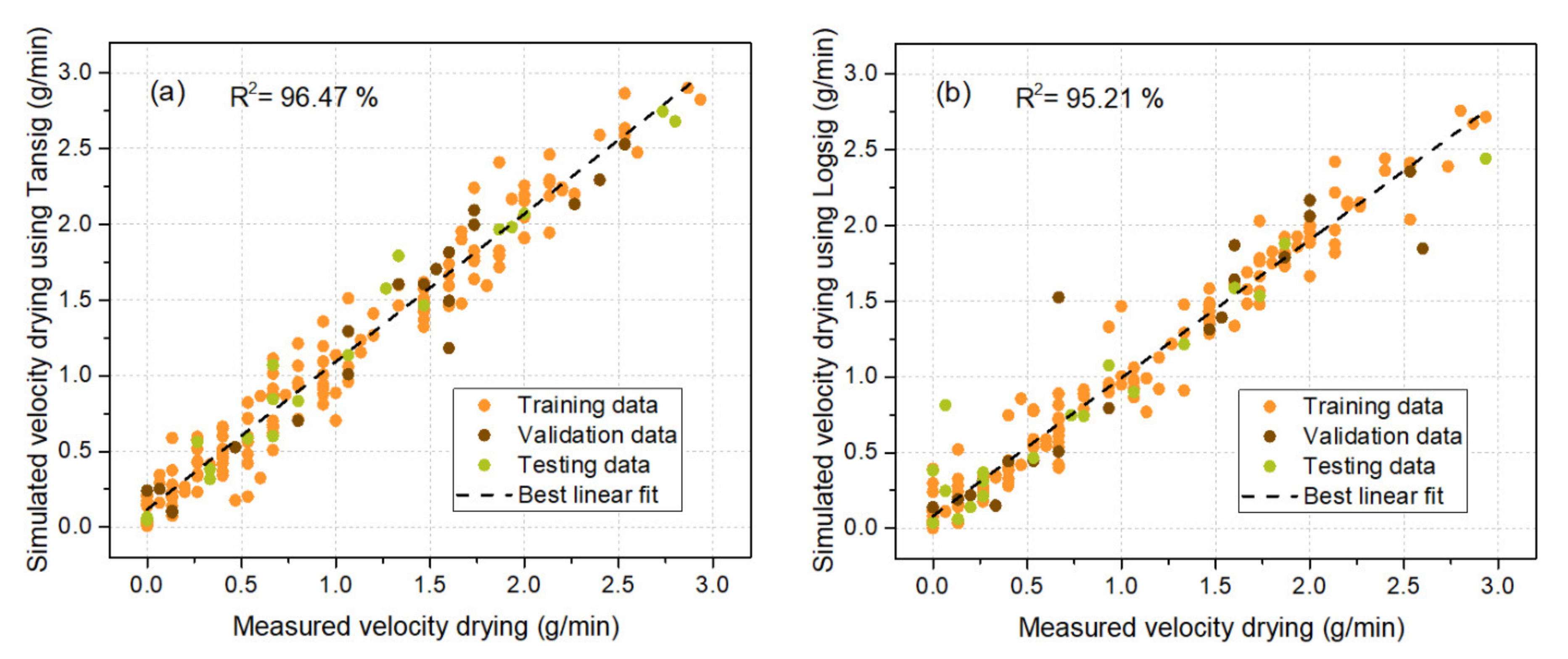
 R = 1 i = 1 n x o u t , e x p i x o u t , s i m i 2 i = 1 n x o u t , e x p i x ¯ o u t , e x p 2
Table 5. ANN network results using the hyperbolic tangent and logistic sigmoid transfer function in the hidden layer.
FunctionArchitecture ANNRMSER2RMAPE (%)Regression Line Equation
Hyperbolic tangent 7–2–10.32150.90520.951460.1 v d , s i m = 0.8637 v d , e x p + 0.3047
7–4–10.26110.91740.957837.0 v d , s i m = 0.9377 v d , e x p + 0.0727
7–6–10.23310.93840.968744.1 v d , s i m = 0.9643 v d , e x p + 0.0955
7–8–10.19120.96470.982231.9 v d , s i m = 0.9865 v d , e x p + 0.1000
7–10–10.17180.96720.983531.5 v d , s i m = 0.9641 v d , e x p + 0.0906
Logistic sigmoid7–2–10.30960.88960.943249.6 v d , s i m = 0.8304 v d , e x p + 0.1417
7–4–10.33770.88020.938252.6 v d , s i m = 0.8331 v d , e x p + 0.0665
7–6–10.30200.91110.954545.8 v d , s i m = 0.8568 v d , e x p + 0.0327
7–8–10.21390.95210.975725.4 v d , s i m = 0.8704 v d , e x p + 0.1169
7–10–10.24670.94300.971137.4 v d , s i m = 0.8903 v d , e x p + 0.0127
Table 6. Weighting and bias parameters obtained for the best ANN model.
Number of Neurons (s) aWeightsBias
Hidden Layer (s = 8, k = 7) IW (s,k)Output Layer (l = 1) LW (s,1)
GT
(k = 1)
Ta
(k = 2)
RH
(k = 3)
wv
(k = 4)
Ti
(k = 5)
To
(k = 6)
Vf
(k = 7)
vd
(s, l)
b1(s)b2(l)
1−1.657−2.9817−2.75132.519314.1473−5.77015.5048−0.9467−4.2106−0.6046
2−4.2833−8.6675−3.15312.81488.0529−4.77813.7780.25347.0302
3−5.44415.19095.2031−1.2298.71260.79225.20290.4303−10.0586
43.87713.30461.0957−4.07552.0218−5.96478.00480.8152−9.7295
5−5.15695.21985.9442−0.798−8.26840.78675.23820.78540.5342
63.98350.0194.3298−4.7365.2334.3233.24960.3684−15.1834
73.4842−3.60184.25514.086112.62890.0656−2.6615−0.0366−14.5054
8−5.6277−1.87473.4161−1.13712.65872.5455−3.68990.025−2.1126
a s is the number of neurons in the hidden layer, k is the number of neurons in the input layer, and l is the number of neurons in the output layer (l = 1).
Table 7. Comparison between experimental data and those obtained from the ANNi model applying the hyperbolic tangent transfer function for taro and plantain.
Experimental
Data
ANNi-GAANNi-PSOANNi-ACO
Vf
(V)
Vf
(V)
Vf
(V)
vd
(g/min)
Vf
(V)
Optimal ε Computing Time (s)Optimal ε Computing Time (s)Optimal ε Computing Time (s)
Taro10.066765.901.673.46.203.333.35.705.004.0
20.933366.172.833.75.754.178.16.203.337.2
31.933366.050.834.36.152.508.66.406.6710.5
42.933365.832.834.56.284.6710.25.754.1710.6
50.133399.33.335.59.353.8911.49.44.4411.5
60.733399.22.224.39.55.568.39.33.3313.7
71.866798.91.113.78.73.337.28.485.7814.2
82.266798.782.443.08.91.118.78.73.3312.0
90.13331211.831.423.211.81.676.811.643.009.2
101.06671211.771.923.512.43.339.511.454.5812.1
Plantain11.86671212.54.174.412.54.178.512.54.1712.0
22.93331212.43.334.311.454.585.212.32.5010.4
30.066766.203.334.96.305.004.15.705.004.1
40.933365.705.005.86.203.334.76.274.505.1
51.933365.685.335.35.832.838.26.152.505.2
62.933366.152.504.45.744.339.76.203.339.6
70.133399.44.443.88.91.1111.38.73.3311.0
80.733398.73.333.88.733.0014.89.44.4415.7
91.866798.812.114.49.44.4416.78.91.1119.0
102.266799.232.564.58.683.5611.88.564.8917.4
Publisher’s Note: MDPI stays neutral with regard to jurisdictional claims in published maps and institutional affiliations.

