Re-Visiting Acoustic Sounding to Advance the Measurement of Optical Turbulence

Abstract

Optical turbulence, as determined by the widely accepted practice of profiling the temperature structure constant, $C_T^2$, via the measurement of ambient atmospheric temperature gradients, can be found to differ quite significantly when characterizing such gradients via thermal-couple differential temperature sensors as compared to doing so with acoustic probes such as those commonly used in sonic anemometry. Similar inconsistencies are observed when comparing optical turbulence strength derived via $C_T^2$ as compared to those through direct optical or imaging measurements of small fluctuations of the index of refraction of air (i.e., scintillation). These irregularities are especially apparent in stable atmospheric layers and during diurnal quiescent periods. Our research demonstrates that when care is taken to properly remove large-scale index of refraction gradients, the sonic anemometer-derived velocity structure constant, $C_v^2$, coupled with the similarly derived turbulence-driven index of refraction and vertical wind shear gradients, provides a refractive index structure constant, $C_n^2$, that can more closely match the optical turbulence strengths inferred by more direct means such as scintillometers or differential image motion techniques. The research also illustrates the utility and robustness of quantifying $C_n^2$ from $C_T^2$ at a point using a single sonic anemometer and establishes a clear set of equations to calculate volumetric $C_n^2$ data using instrumentation that measures wind velocities with more spatial/temporal fidelity than temperature.

1. Introduction

The index of the refraction structure constant, $C_n^2$, is commonly used to quantify optical turbulence strength, which, in turn, can degrade both active and passive system performance, whether that of a laser central to a free space optical communication uplink, an inter-continental relay mirror high energy laser power-beaming architecture to transport energy to remote sites, or an upward-looking telescope pointed at a distant space object. Though valuable and ever more capable, a path-averaged and even a path-resolved measurement of $C_n^2$ is available via optical means such as scintillometry [1] and time-lapse imagery [2,3], respectively. Even so, continuous, high frequency, very localized, point measurement of causative temperature, moisture, and wind gradients near the source or image plane of one’s active/passive system can be difficult using optical means because one is observing a net optical effect. Such localized point measurements, however, are especially beneficial to engineers and scientists who develop and apply compensation and correction techniques and associated modalities, as well as those individuals endeavoring to develop, verify, and validate optical turbulence and effects models through carefully instrumented field tests and post-test forensics analysis. Similarly, these high-fidelity flux measurements are of interest to mission planners and system operators seeking to update/nudge an otherwise long range, days-to-weeks advance forecast of system performance to support up-to-the-minute mission briefs [4] and current-mission system settings. The latter advance forecasts are built on a combination of increasingly sophisticated laser propagation and numerical weather prediction models.

By emphasizing the high frequency measurement of the time of flight of an acoustic pulse transmitted between two probes, 3D sonic anemometers were originally conceived, and subsequently extensively applied, to assess temperature gradients and, thus, the temperature structure constant. However, limiting one’s analysis to temperature gradients can lead to a sub-optimal assessment of optical turbulence strength during, for example, diurnal quiescent periods. During these periods, temperature gradients in all directions diminish to near zero—the evening quiescent period ends because the ground (due to radiative losses to space) cools the air near it and creates a vertical temperature gradient, and as the night goes along, horizontal gradients are established because of different cooling rates of different surfaces. The morning quiescent period breaks down because of the opposite effect of the sun heating the ground. At night (in stable conditions), waves along the stable layers—caused by wind and large object movement—create a spatial and temporal index of refraction fluctuations that create “optical turbulence” effects on laser/optical propagation. During the day, the sun heating the ground creates convection that supports more statistically characterize-able advecting turbulent eddies (e.g., Kolmogorov turbulence) that produce a spatial and temporal index of refraction fluctuations that, in turn, effect electromagnetic—especially optical and near infrared—wave propagation in the classical “optical turbulence” way. While temperature gradients are, in general, the largest contributor to the index of refraction gradients, humidity gradients and pressure perturbations also contribute. Calculating $C_n^2$ from $C_T^2,$ in some cases, makes quiescent periods seem far more marked than they often are as measured by an optical instrument such as a scintillometer. Arrays of sonic anemometers measure the speed of sound in air in many directions, thus, they can conceivably capture gradients in the temperature, humidity (since this affects air density and the speed of sound), and the velocity. The velocity fluctuations are created by the small turbulent eddies or waves on the stratified layers that have small circulations (e.g., vortices) associated with them, which, in turn, produce pressure/density gradients that establish an index of refraction gradients with very little temperature change. These humidity and pressure/density variations often continue to exist during quiescent periods and in adiabatic layers, keeping actual $C_n^2$ levels significantly higher than those characterized through a consideration of $C_T^2$ only. This suggests the rationale for employing arrays of sonic anemometers as control research and test instrumentation to capture more fully the physics that create optical turbulence effects.

This study demonstrates the implementation of 3D sonic anemometers arrayed in a way to do what each sonic anemometer was originally designed to do best: acoustically interrogate eddies and sense temperature, moisture, and wind velocity (and hence pressure) gradients, which, in combination, lead to index of refraction gradients. Nosov et al. [5] have similarly demonstrated a calibrated method to obtain $C_T^2$, $C_v^2$, and $C_n^2$ from a small array of ultrasonic anemometers. This paper extends the relationships shown in [5] with evidence demonstrating optical turbulence strength, $C_n^2$, can be derived from a parameter, $C_v^2$, which is more directly tied to the turbulent eddy distribution independent of non-adiabatic temperature gradients that many techniques tend to exploit to their advantage, but that can disappear when turbulence does not. Shikhovtsev et al. [6] have noted the potential importance of quantifying the non-temperature gradient component that partially drives turbulent eddy production with their seasonal study of $C_n^2$ strength near Lake Baykal that peaked in winter when winds are strongest. While underlining the benefits of employing local sonic anemometer arrays, this paper also seeks to set forth a solid set of relationships of equal relevance when one is using acoustic sounding—whether sonic anemometry or other familiar techniques such as Sound Detection and Ranging (SODAR)—to evaluate and characterize optical turbulence. A validation of these relationships will primarily be accomplished through a comparative evaluation of the results obtained through path-resolved optical means. Materials and Methods for the present work are described in Section 2. This section derives, or when of common usage simply references, the key physical expressions enabling an investigation of optical turbulence strengths and effects using acoustically observed micro-meteorological parameters. Section 2 also provides a description of the sonic anemometer arrays, supporting instrumentation, and the general field experiment set-up. It is in this section that the equivalency of the sonic and virtual temperature is demonstrated (they have previously been assumed different but approximately equal), and a new method to remove the non-turbulent layer vertical temperature change that is independent of atmospheric stability is introduced. Furthermore, a summary description of a path-resolved optical turbulence profiler used for comparative reference is included here as well. Representative optical turbulence point measurements, as collected from sonic anemometers installed on a static tower, will be profiled, analyzed, and comparatively evaluated with the reference path-resolved optical turbulence measurements in Section 3. Section 4 will conclude by summarizing the analysis and discussion of the preceding section, the implications of the findings, and future research directions.

2. Materials and Methods

2.1. Structure Parameters

In their widely acknowledged development of atmospheric electromagnetic wave propagation amidst fluctuations associated with the temperature, moisture, and pressure, Kolmogorov and then Tatarskii advanced the concept of structure functions. In combination, this led to an analytical basis for quantifying optical turbulence, the correlation of the associated random localized small-scale fluctuations of the former physical parameters, the spatial/temporal characteristics of turbulent eddies in the atmosphere, and, subsequently, the effects on the index of refraction [7,8]. In those instances where the turbulent flow can be characterized as Kolmogorov—isotropic, homogenous, and an associated energy spectrum falling within the inertial sub-range where energy is neither created nor dissipated by the large and small eddies—the structure function is described according to the Kolmogorov–Obhukov two-third power law. For the sake of illustration, to account for temperature fluctuations, the structure function, $D_T$, is expressed as follows [7]:

$$D_T\left(r\right)=\langle {\left[T\left(r_2\right)-T\left(r_1\right)\right]}^2\rangle =C_T^2{\left|r_2-r_1\right|}^{2/3}$$

(1)

where $C_T^2$ is the structure parameter for temperature,$T$, and the brackets, $\langle .\rangle$, signify an ensemble average. The underlying analytical theory presumed temperature measurements at two points separated by the distance $r$. In practice though, such micrometeorological parameters are generally measured at a single point as a function of time, $t$. In order to correlate these temporally varying point measurements to spatial variability in temperature, Taylor’s frozen turbulence hypothesis generally is invoked. Taylor’s hypothesis postulates the shapes of the turbulent eddies is frozen in time and move perpendicularly past a probe or observer at the convection velocity, $\langle V_{\perp }\rangle$, which for Taylor’s frozen turbulence hypothesis is taken as equivalent to the local mean wind velocity. Subsequently, Equation (1) can be re-written as follows:

$$C_T^2={\langle \left[T\left(t+\mathsf{\Delta }t\right)-T\left(t\right)\right]\rangle }^2{\left(\langle V_{\perp }\rangle \mathsf{\Delta }t\right)}^{-2/3}$$

(2)

Kaimal and Finnigan [9] (pp. 61–62), however, counter the tenets of this hypothesis through references to field studies that demonstrated larger eddies moved faster than their smaller counterparts. Naturally, such a variable flow and consequent non-uniform momentum, heat, and mass transfer throughout the atmosphere, especially in the mixed atmospheric boundary layer, lead one to discount assumptions of frozen eddy shapes and sizes. Nonetheless, this reference argued as convincingly that such assumptions have been validated through a large number of observations and associated time-averaged statistics. Additionally, many measurements, such as those recorded with sonic anemometers, are conducted at extremely high frequencies, wherein eddies are not likely to change over the course of the measurement period.

Specific to optical turbulence and its effects on electromagnetic wave propagation, the causal index of refraction fluctuations are characterized by the structure parameter for the index of refraction, which can be expressed in a form similar to Equation (2) but with regard to each of the physical scalars influencing the atmospheric index of refraction—temperature, moisture, and pressure. In large part, though, scientists and engineers characterizing atmospheric and optical turbulence effects in the visible and near infrared are satisfied with the following straightforward expression tying $C_n^2$ to $C_T^2$:

$$C_n^2={\left(79.2\times {10}^{-6}\frac{P}{T^2}\right)}^2{C}_T^2$$

(3)

where $P$ is pressure (hPa) and $T$ is the ambient air temperature (K). This expression was originally derived from first principles and presented by Tatarskii [8] (p. 102) but was also arrived at through empirical measurement of fine scale temperature fluctuations in the course of optical experiments [10]. Several key assumptions underlie the application of Equation (3) [11]. These include statistically homogeneous and isotropic Kolmogorov turbulence; moisture fluctuations are of small consequence in both the optical (visible) and near infra-red portions of the spectrum, which generally is acknowledged as reasonable except over water surfaces [12]; and pressure fluctuations that are presumed to rapidly dissipate as compared to the temperature fluctuations, and generally thought to be inconsequential. Interestingly then, though it is widely known that the original theory underpinning optical turbulence and its effects originated with regard to velocity fluctuations (pulsations) [7], the velocity structure constant is not explicitly represented in Equation (3). Indeed, very satisfactory results have been obtained by simply calculating $C_T^2$ using two high-speed, fine-wire thermometers to record temperature fluctuations as a function of time. With comparable accuracy, 3D sonic anemometers have also been used extensively to record temperature fluctuations [13]. Yet, for instances of neutral stratification, $C_T^2$ will trend towards zero, and one would presume optical turbulence strengths would trend likewise. However, observations of such tendencies, as might be anticipated during the diurnal quiescent periods after sunrise or before sunset or on windy or cloudy days, have not been so absolute [14]. Tatarskii’s original development attempted to quantitatively characterize optical turbulence even for these instances of neutral stratification by accounting for the vertical gradients in wind velocity, pressure, and moisture, as well as temperature—which led to fluctuations in the index of refraction and its structure constant [8]. As will be discussed shortly, sonic anemometers are inherently designed to measure speed of sound fluctuations caused by moisture, temperature, and velocity fluctuations and, hence, pressure fluctuations. Turbulent eddies, each with characteristic moisture, temperature, and pressure, cross the sonic anemometer’s acoustic propagation path at a velocity linked to that of the localized mean wind velocity as well as fluctuations in the flow’s velocity. In fact, Bernoulli’s principle suggests the latter fluctuations can lead to pressure fluctuations. These velocity fluctuations can be characterized according to a derived structure parameter for velocity.

As earlier, assuming Kolmogorov turbulence and Taylor’s frozen turbulence hypothesis, the velocity structure parameter, $C_v^2$, which characterizes the eddy and turbulent flow’s velocity fluctuations, can be written as follows [11]:

$$C_v^2={\left[V_{\perp }\left(t+\mathsf{\Delta }t\right)-V_{\perp }\left(t\right)\right]}^2{\left(V_{\perp }\mathsf{\Delta }t\right)}^{-2/3},$$

(4)

where $V_{\perp }$ represents the measurement of the velocity fluctuations transverse to the field instrumentation’s characteristic observation path(s). Returning to Kolmogorov’s original derivation, where $C_v^2$ was shown to describe the turbulence flow’s total energy, an explicit expression showing the link between $C_n^2$ and $C_v^2$ is derived in Appendix A and is as follows:

$$C_n^2=1.4C_v^2{\left[\nabla \langle n\rangle /\left(\partial \langle \mathit{V}\left(z\right)\rangle ⁄\partial z\right)\right]}^2,$$

(5)

where $\nabla \langle n\rangle$ is the gradient of the ensemble average of the fluctuations of the index of refraction, and $\partial \langle \mathit{V}\left(z\right)\rangle ⁄\partial z$ is the ensemble average of the vertical gradient of the wind velocity fluctuations. As will be made clear shortly, this result accounts for fluctuations in temperature as well as moisture, by way of $\nabla n$. This expression brings forward the centrality of the turbulent flow’s velocity gradients and fluctuations, which anchored Obhukov, Kolmogorov, Tatarskii, and others’ optical turbulence theory. The expression in Equation (5) also leads one to consider an alternative point measurement approach wherein one exploits sonic anemometery, positioning a primary and secondary sonic anemometer vertically one above the other, to derive the requisite gradients between two layers, while simultaneously evaluating $C_v^2$ at the primary point of interest.

2.2. Sonic Anemometry and Optical Turbulence Point Measurement

For 3D sonic anemometers, the characteristic observation paths include three axial piezo-electric transducers pairs, each transducer probe emitting ultra-short, very high frequency, acoustic signals in unison with its partner, and then recording the time delay difference between the transmitted and received acoustic signals. In sum, six acoustic signals will have travelled through an air parcel moving across the fixed transducer separation paths with a velocity governed by that parcel’s characteristic horizontal (“u” and “v”) and vertical “w” wind velocity. The time delay difference will also be influenced by the speed of sound, which for ambient air can be expressed by adapting the ideal gas law to account for water vapor via the parcel’s virtual temperature (the temperature at which a dry air parcel has the same density as its moist counterpart held at the same pressure), as follows:

$$c={\left({\gamma }_{d}P/\rho \right)}^{1/2}={\left({\gamma }_d{R}_d{T}_v\right)}^{1/2}={\left({\gamma }_d{R}_d{T}_v\right)}^{1/2},$$

(6)

where $c$ is the velocity (m/s) of sound in ambient air, $P$ is the absolute air pressure (Pa), $\rho =P/R_d{T}_v$ is an expression for the density $\left(kg/m^3\right)$ of a moist air parcel, $T_v$ is the parcel’s virtual temperature (K), and ${\gamma }_d$ (1.4) and $R_d \left(287 J/kg·K\right)$ are the standard dry air specific heat ratio and gas constant, respectively. In practice, meteorologists define and approximate $T_v$ as follows:

$$\begin{gathered} T_v=T\left[1+0.61q\right]=T\left[1+0.61\left(\frac{\mathsf{\epsilon }e}{P-0.378e}\right)\right]\approx T\left[1+0.61\mathsf{\epsilon }\frac{e}{P}\right] \\ \approx T\left[1+0.38e/P\right], \end{gathered}$$

(7)

where $q$ is the specific humidity (the mass of water vapor per unit mass of the moist air parcel sampled), $\mathsf{\epsilon }$ is the ratio of the molecular masses of water vapor and dry air (i.e., 0.622), and $e$ is the vapor pressure (Pa). Thus,

$$c\approx {\left({\gamma }_d{R}_{d}T\left[1+0.38e/P\right]\right)}^{1/2}$$

(8)

Alternatively, it is common practice among those using sonic anemometers to express $c$ as follows [15,16]:

$$c={\left({\gamma }_d{R}_{d}T\left[1+0.51q\right]\right)}^{1/2}\approx {\left({\gamma }_d{R}_{d}T\left[1+0.32e/P\right]\right)}^{1/2},$$

(9)

where the sonic temperature, $T_s$, is often referred to as the sonic virtual temperature, and defined as follows:

$$T_s=T\left[1+0.32e/P\right]$$

(10)

Through investigation, Kaimal and Gaynor [16] identified the source for the difference between the sonic virtual temperature (Equation (10)) and meteorological virtual temperature (Equation (7)). The distinction originated in the leading coefficient to the ratio of $e/P$, where that for Equation (7) is effectively $\left(1-M_w/M_a\right)$ and that for Equation (10) is derived from $\left({\gamma }_w/{\gamma }_a-M_w/M_a\right)$, in which ${\gamma }_w/{\gamma }_a$ is the ratio of the specific heat ratios of water vapor and dry air $\left(1.33/1.4\right)$ and $M_w/M_a$ is the ratio of the molecular masses of water vapor and dry air (0.622) [17]. This effectively adjusts the 0.61 coefficient in Equation (7) to 0.51 in Equation (9). However, this explanation appears to ignore that $q\approx \mathsf{\epsilon }e/P$ is itself an approximation (the left side of Equation (7) captures the definition of specific humidity) that slightly underestimates the value of q, especially in very moist air. This suggests that the 0.32 coefficient that appears in Equations (9) and (10) should be larger, and perhaps closer to the 0.38 value that appears in Equations (7) and (8). Furthermore, Fleagle and Businger [18] show that the effect of water vapor content on the dry air values of the specific heat at constant pressure (c_p) and constant volume (c_v) can be quantified as follows:

$$\begin{gathered} c_p=\left(1+0.84q\right)c_{pa} \\ {c}_v=\left(1+0.93q\right)c_{va}, \end{gathered}$$

(11)

where c_pa = 1005 J kg⁻¹ K⁻¹ and c_va = 718 J kg⁻¹ K⁻¹ are the dry air values of the specific heats and q is, again, the specific humidity. When the air is 100% water vapor, q = 1 and Equation (11) provides the specific heat values for pure water vapor, c_pw = 1847 J kg⁻¹ K⁻¹, c_vw = 1386 J kg⁻¹ K⁻¹, and ${\gamma }_w/{\gamma }_a=1.33/1.4$. However, air in the free atmosphere rarely exceeds about 2% water vapor content by mass; with q = 0.02—which is equivalent to a near sea level dew point temperature of ~300 K—${\gamma }_w/{\gamma }_a=1.39/1.4\approx 1$. Thus, the leading coefficient to the ratio of $e/P$ is effectively only $\left(1-M_w/M_a\right)$. Accordingly, it had become common practice to assume that the sonic virtual temperature very closely approximates the meteorological virtual temperature and can for all intents and purposes be treated as equivalent; the arguments herein remove any concern about the equivalency of these two parameters. The virtual temperature simplifies the treatment of moisture contributions to many local atmospheric processes including buoyancy and index of refraction gradients, which will be discussed further below. In sum, the sonic virtual temperature, derived through processing of time-delayed acoustic wave propagation, provides ready-access to the meteorological atmospheric virtual temperature. The virtual temperature, in turn, provides a means to quantify the local index of refraction’s dependence on both temperature and moisture.

Returning to Equation (5), while the results for $C_v^2$ and $\partial \langle \mathit{V}\left(z\right)\rangle ⁄\partial z$ are regularly retrieved directly from the sonic anemometer outputs, those for the gradient of the index of refraction, $\nabla n$, require consideration of the contributing factors. Beginning with Tatarskii, the potential temperature (really the potential virtual temperature)—a conserved quantity—naturally is referenced quite frequently when attempting to infer or evaluate the latter gradient [8,19,20]. With the advent of new optical techniques to deduce the index of refraction fluctuations, some have chosen $T_v$ as an alternative to using a conservative quantity to assist with quantifying these fluctuations through optical measurements [21]. By opting to take the alternative path, separately obtaining accurate water vapor fluctuation measurements is not necessary since the moisture quantification is contained in the virtual temperature. Proceeding in this manner, one begins by selecting an expression for air’s index of refraction. Given its lineage, an attractive option is that developed by Edlen, which culminated in what has been labelled as modified-Edlen or Edlen66 [22]. Amongst other enhancements, Edlen66 accounted for the refractivity of water vapor. Consistent with the development’s underlying principle, the air’s refractive index is linked to its density according to the following:

$$n-1=a\rho ,$$

(12)

where, according to Edlen66 with air density normalized to 1 kg-m⁻³ [22],

$$\begin{gathered} n-1={10}^{-6}\left[83.4212+24060.3/\left(130-1/{\lambda }^2\right) \\ +159.97/\left(38.9-1/{\lambda }^2\right)\right] \end{gathered}$$

(13)

On combining Equations (12) and (13), one can solve for $a$, which is found to be 0.227 × 10⁻³ m³-kg⁻¹ for visible light ($\lambda =0.550 \mu$m) for a standard atmosphere at sea level where the air density is 1.225 kg-m⁻³. Consequently, for an air parcel displaced from level $z_1$ to level $z_2$, the gradient of the displaced parcel’s index of refraction can be approximated as follows:

$$\nabla n_{z_1\to z_2}=\overline{\rho }\frac{\partial a}{\partial z}+a\frac{\partial \rho }{\partial z}\approx a\frac{\partial \rho }{\partial z},$$

(14)

where the first term in Equation (14) is, by Edlen’s premise, zero: $a$ is normalized to air density. As introduced earlier, a modified form of the ideal gas law can be written as $\rho =P/R_d{T}_v$ to account for moisture, which results in the following:

$$\nabla n_{z_1\to z_2}\approx a\frac{\partial \rho }{\partial z}\approx \frac{a}{R_d\overline{T_v}}\left[\frac{-\overline{P}}{\overline{T_v}}\left(\frac{\partial T_v}{\partial z}\right)+\left(\frac{\partial P}{\partial z}\right)\right],$$

(15)

Recalling that $\partial P/\partial z=-\rho g$, where $g$ is the acceleration due to gravity, one can re-write Equation (15) as follows:

$$\nabla n_{z_1\to z_2}\approx \frac{-a\overline{P}}{R_d{\overline{T_v}}^2}\left[\frac{\partial T_v}{\partial z}+\frac{g}{R_d}\right]\approx \frac{-a\overline{\rho }}{\overline{T_v}}\left[\frac{\partial T_v}{\partial z}+\frac{g}{R_d}\right]\approx \frac{-\left(n-1\right)}{\overline{T_v}}\left[\frac{\partial T_v}{\partial z}+\frac{g}{R_d}\right],$$

(16)

As developed earlier in this paper, $T_v$ is effectively the sonic temperature recorded using the sonic anemometer. It is not a conserved quantity as is the potential virtual temperature. In order to discern the dynamic range of the fluctuations in the index of refraction gradient, as is implied in the derivation associated with Equation (5), converting to a potential virtual temperature is warranted, but not necessary if one removes the large-scale virtual temperature lapse rate with height. However, to ensure consistency and preserve the underlying nature of the causal source of the gradients (i.e., turbulent mixing), the gradient of the index of refraction can be separated into a large-scale index component—an ensemble average—and an eddy component that represents the small-scale turbulent fluctuations as follows:

$$\nabla n=\nabla n+\nabla n^{\prime }$$

(17)

By doing so, the dominant large-scale index of refraction gradients, otherwise concealing high frequency (small-scale) fluctuations in the index of refraction gradient that determine $C_n^2$, can be removed to arrive at the following:

$$\nabla n_{z_1\to z_2}^{\prime }\approx \left\{\frac{-\left(n-1\right)}{\overline{T_v}}\left[\raisebox{1ex}{$\partial T_v$}\!\left/ \!\raisebox{-1ex}{$\partial z$}\right.+\raisebox{1ex}{$g$}\!\left/ \!\raisebox{-1ex}{$R_d$}\right.\right]\right\}-\left\{\frac{-\left(n-1\right)}{\overline{T_v}}\left[\raisebox{1ex}{$\partial T_v$}\!\left/ \!\raisebox{-1ex}{$\partial z$}\right.+\raisebox{1ex}{$g$}\!\left/ \!\raisebox{-1ex}{$R_d$}\right.\right]\right\}$$

(18)

By assuming the mean layer virtual temperature at any one time, $\overline{T_v}$ is equivalent to the ensemble average mean layer virtual temperature, $\langle \overline{T_v}\rangle$, Equation (18) can be simplified to the following:

$$\nabla {n^{\prime }}_{z_1\to z_2}\approx \frac{-\left(n-1\right)}{\langle \overline{T_v}\rangle }\left[\frac{\partial T_v-\partial \langle T_v\rangle }{\partial z}\right]$$

(19)

The ensemble average of the right side of Equation (19) provides $\nabla \langle n^{\prime }\rangle$, which is then combined with the other terms in Equation (5) to arrive at a $C_n^2$ profile.

2.3. Path Resolved Optical Turbulence Profiler for Comparative Reference

The Delayed Tilt Anisoplanatism (DELTA) instrument shown in Figure 1 is a turbulence profiling system developed by MZA [23]. The DELTA system uses an 8-inch aperture to image a distant target onto a science camera. Images are captured at 100 frames per second. The system measures the differential motion, or tilts between pairs of feature points on the target as a function of their angular separation. The differential tilt variance between a pair of feature points is a path-weighted integral of $C_n^2$. Figure 2 shows the target board used for DELTA measurements in the present work and weighting functions for differential tilt variances, corresponding to four different feature point separations on the target board. These weighting functions drop to zero at both ends of the path. Sub-aperture separations have weighting functions with peaks closer to the source end of the path. Weighting functions for large separations have peaks closer to the aperture end of the path. The DELTA processing software uses the measured differential tilt variances for various separations, along with the corresponding weighting functions to generate turbulence profiles along the path. Turbulence values are typically reported in 10 bins distributed along the path. Frames captured during a three second window are used to generate a turbulence profile. Turbulence parameters such as Rytov number, Fried’s coherence diameter, Scintillation index as well as crosswind speeds are calculated from this profile. The maximum operational range for a DELTA system is approximately two kilometers.

When turbulence is strong, the feature points on the target become blurry and can no longer be tracked as points. While trying to still track feature points, DELTA measures smaller differential tilt variances due to the blurring. This leads to an underestimation of $C_n^2$ values during periods of strong turbulence. Since DELTA measures differential motion between feature points, the whole image shift, due to changes in the large-scale refractive index gradient, does not affect the measurements.

2.4. Field Test Description: Propagation Path and Instrumentation Bed-Down

Section 3 below presents optical turbulence profiles derived by in situ micro-meteorological point measurements recorded using two time-synchronized sonic anemometers, one designated as primary and the other secondary, installed at arbitrary heights, $z_1$ and $z_2$, vertically one above the other. Being vertically stacked, the associated sonic anemometer stations are hereafter referred to as stacked sonic anemometer masts. Subsequently, a diurnal, temporally varying optical turbulence profile at a primary point and height of interest is derived using Equation (5) above. Namely, the profile is arrived at by combining the wind velocity and calculated small scale fluctuations of the index of refraction gradients between the secondary and primary level with the velocity structure constant as derived using the primary instrument’s measurements. As the sonic anemometers are installed one directly above the other to ensure there is no lateral offset, the gradients essentially are with respect to the vertical direction. As reference, the primary sonic anemometer’s recorded temperature fluctuations are used to calculate the temperature structure function at the primary point of interest, and hence profile optical turbulence using the standard approach through the application of Equation (3). Given the 10 Hz sampling rate of the sonic anemometers, a 90-second ensemble averaging time was largely utilized for the presented results because $C_n^2$ profiles obtained via Equation (5) and those obtained via optical methods and $C_T^2$ converged best in terms of variability and magnitude. It is also close to the 100-second ensemble averaging time suggested in [5]. The selection of optimum ensemble averaging times, especially when pursuing the technique presented here, would likely benefit from further investigation.

The field measurements were conducted at Wright Patterson AFB, Ohio during the summer of 2020 and the height of the COVID-19 pandemic. Atmospheric micrometeorological as well as soil measurements were recorded at multiple points along a 1.9-kilometer propagation path. While the slant path traversed many types of soil/canopy cover and topographical features, equipment and personnel availability limited the deployment of stacked sonic anemometer masts to two locations along the path. An aerial view of the slant path and surrounding area is shown in Figure 3 along with the locations of the stacked sonic anemometer mast stations.

A portion of the propagation path was situated alongside the quasi-active runway-taxiway used to fly in aircraft for display at the National Museum of the United States Air Force. The topography, a portion of which is level and open, can lead to strong wind shears, and indeed one of the Dayton area tornados of May 2019 had passed through this area. Sonic anemometry continues to benefit from a strong vendor base, which makes high-quality instrumentation and a wide variety of probe array configurations available, many optimized according to one’s application (e.g., optical imaging and communication, near-surface fundamental eddy covariance flux assessments, or canopy wind effects and simulations). Others are designed to operate well in extreme ambient conditions (i.e., some probes are configured for especially high wind velocity), and/or to minimize flow asymmetries and interference associated with towers and other structures on which the sonic anemometers are mounted. For this research, a variety of probe configurations designed and built by Applied Technologies Inc. (ATI) were considered and fielded, amongst which is ATI’s non-orthogonal A-probe. This probe’s specifications include the ability to preserve sonic temperature and wind velocity precision and accuracy even in conditions of very high wind speeds.

Ultimately, the best correlated, multi-instrument dataset for the study herein occurred during a 2-day period of benign weather: 14–15 July 2020. Conditions during this period were near 30-year climatological means. On 14 July, the sky condition was clear to partly cloudy, temperatures varied from 17 to 30 °C, with light east to northeast winds, and a period of no wind from ~0200UTC to 1200UTC where a significant temperature inversion near the surface occurred. On 15 July, the sky condition was nearly clear all day, temperatures varied from 19 to 32 °C, with light south to southwest winds, and periods of calm from ~0200UTC to 1200UTC. Dew point temperatures remained between 15 to 18 °C for the entire 2-day period; this means relative humidity varied from ~30% in the afternoons to ~90% in the mornings just before sunrise.

2.5. Data Analysis: Summary Description

The relevant structure functions were calculated in the spatial domain using the recorded measurements in their raw form as opposed to implementing an intermediate step converting the data to the frequency domain. Additionally, given the topographical non-homogeneities and acknowledging the challenges associated with precision leveling and alignment of a single sonic anemometer, much less a coupled pair, stream-wise rotation was applied to the sonic anemometer velocity measurements [24].

3. Results and Discussion

The top set of plots in Figure 4 shows calculated $C_n^2$ profiles for 14 July 2020 that originated from $T_s$ measurements recorded using the ATI sonic anemometers mounted at 6.4, 10.2, and 24.5 m above the surface. The profiles are a direct result of calculation of the structure function $C_T^2$ according to Equation (2) and then through application of Equation (3). These profiles show typical quiescent periods at approximately an hour after sunrise (1130UTC) and an hour prior to sunset (2330UTC). Generally, the highest anemometer recorded the lower $C_n^2$ values, while the lowest anemometer recorded the highest values. Of note are the periods where this general characteristic is reversed (e.g., ~0500 to ~0730UTC); these are periods of marked atmospheric stability.

The bottom set of plots shown in Figure 4 illustrate the importance of removing the large-scale index of refraction and only using the portion of the refractive gradient that is driven by turbulence (i.e., the small-scale fluctuations in the index of refraction gradient $\nabla$n’, per Equation (19)). The 24.5-meter $C_n^2$ from the $C_T^2$ plot in the bottom portion of Figure 4 is the same as the 24.5-meter plot shown in the top portion of the figure, except that a 90-second ensemble averaging time is used instead of 180 s; this $C_n^2$ from the $C_T^2$ profile was used as a reference to verify the suitability of the $C_n^2$ from the $C_v^2$ calculation. Subsequently profiled in the bottom portion of Figure 4 are $C_n^2$ from $C_v^2$ using alternate forms of the temperature gradient when deriving the vertical gradient of the index of refraction. The $C_n^2$ from $C_v^2$ using T_v for the vertical temperature gradient (∂T_v/∂z) plot deviates significantly from the $C_n^2$ from $C_T^2$ baseline plot during quiescent periods, stable periods, and the late afternoon—virtually throughout the entire period. This is expected, since ∂T_v/∂z contains the temperature decrease with height caused by air expanding adiabatically—this is the primary component of the large-scale index of refraction that is always present in the atmosphere to some degree and is not due to turbulence and the index of refraction structure function. A common practice to remove this adiabatic expansion cooling effect is to convert the temperature or virtual temperature to potential temperature or potential virtual temperature as conducted in the Appendix A to arrive at Equation (5). This was conducted for the $C_n^2$ from $C_v^2$ using the potential virtual temperature, θ_v, for the vertical temperature gradient (∂θ_v/∂z)—and hence the index of refraction gradient—plot in the lower part of Figure 4. While this brought the $C_n^2$ from $C_v^2$ using the ∂θ_v/∂z plot much more in line with the $C_n^2$ from the $C_T^2$ baseline plot, there remained a significant deviation during the stable period from ~0500UTC to ~0730UTC when θ_v increased with height. Using ∂θ_v/∂z for the lapse with height should have corrected the $C_n^2$ from the $C_v^2$ plot to the baseline at all times. However, it did not because an accurate conversion from T_v to θ_v requires the instantaneous pressure value associated with each sonic T_v measurement at each level utilized in the ∂θ_v/∂z calculation. Since the sonic anemometers did not provide instantaneous pressure measurements with each T_v value, the pressure was calculated at the level of each sonic anemometer from the pressure at the level of the DELTA target board weather station assuming hydrostatic balance. This produced a dry adiabatic lapse of temperature and introduced large-scale index of refraction ∂θ_v/∂z errors at times when the atmosphere was markedly stable (not adiabatic). Thus, this research presents the methodology encapsulated in Equations (17)–(19) whereby the large-scale T_v vertical gradient, and, in turn, the large-scale index of refraction gradient, is removed without the need for instantaneous pressure at each sonic T_v measurement. The impact is quite apparent. As can be seen in the bottom part of Figure 4, the $C_n^2$ from $C_v^2$ with the large scale T_v vertical gradient removed plot follows the $C_n^2$ from the $C_T^2$ baseline plot throughout the entire day.

Figure 5 shows the calculated $C_n^2$ profiles for 14 July 2020 at 24.5 m above the surface predicated on a calculation of the velocity structure constant, $C_v^2$, at that height as well as the ensemble average of the small scale fluctuations of the index of refraction gradient, $\nabla n^{\prime }$, and the ensemble average of the gradient of the wind velocity in the vertical direction $\partial \langle \mathit{V}\left(z\right)\rangle ⁄\partial z$. As described in Section 2, the latter gradients are determined via measurements recorded with a primary and secondary sonic anemometer, in this case the primary was at 24.5 m above the ground and the secondary at 10.2 m above the ground. The calculations were implemented after converting the primary and secondary sonic anemometer velocity measurements to the mean wind streamlined coordinate system through triple rotation about the sonic anemometer’s u, v, and w coordinate system summarily referenced in Section 2.5 above. Figure 5 also includes the $C_n^2$ profile as derived from $C_T^2$. The correlation is quite good.

In turn, Figure 6 and Figure 7 show the effect of the streamwise rotation of the wind vector, wherein the sonic anemometer data is treated in a streamlined coordinate system.

The impact of streamwise rotation is especially significant for the measurements nearer the surface (i.e., at 10.2 m), which is to be expected given the increased proximity to topographical inhomogeneities at the lower height.

The profiles of $C_n^2$ at both 24.5 and 10.2 m for July 14 are overlaid in Figure 8. As is the case in Figure 6 and Figure 7 above, each profile at the height of interest is obtained by combining the wind velocity and calculated small scale fluctuations of the index of refraction gradients with the velocity structure constant, C_v, using the primary sonic anemometer’s (whether at 24.5 or 10.2 m) point measurements. There is no discernible difference in the magnitude of the $C_n^2$ at each level in Figure 8, as is evident in the top image of Figure 4; this is likely due to the turbulent refractive index gradient in the 10.2 to 24.5 m layer being the primary calculation component for the $C_n^2$ at both levels.

In Figure 9, the DELTA $C_n^2$ profile overlays those of the sonic anemometers quite well through the day, even at the sunset/sunrise quiescent periods, though there is a notable separation at approximately 1700UTC to 2400UTC. The DELTA’s lower afternoon $C_n^2$ values brought its mean $C_n^2$ value for the day to less than half the mean value found using both sonic anemometer methods. Examining the DELTA camera images shown in Figure 10 below seems to suggest this separation occurred as the target board’s feature points became more difficult to discern and track, specifically from approximately 1700UTC through 2100UTC, when the target board became more backlit as the sun transited to the western portion of the sky. Additionally, the 14/0006UTC image in Figure 10 shows that the target board illumination that was used during the field test appears to overwhelm the near sunset lighting conditions causing such a high contrast that only large feature separation distances are discernible. 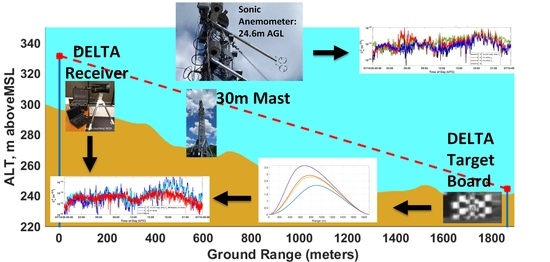This could have had the effect of limiting the number of weighting functions such that the DELTA would provide more of an integrated path $C_n^2$ value weighted slightly toward the camera end of the path—which was 30 m high on a 60-meter tower. This increases the likelihood that the DELTA and 30-meter mast sonic anemometer instruments were sampling significantly different volumes of air. The 14/1200UTC image in Figure 10 shows the target board clearly displayed many different feature separations such that the full number of weighting functions—including one peaking near the 600-meter distance from the DELTA receiver to the 30-meter mast—should have been available for a true profiling capability. Additionally, it is evident in Figure 10 that the target board position shifted significantly in the images throughout the day, this had little consequence on the system’s ability to quantify and profile turbulence along the path since multiple feature separation distances were always visible within the camera’s processing “mask” field of view. Thus, the DELTA $C_n^2$ profile measurement method is not susceptible to large-scale effects on the $C_n^2$ quantification since DELTA only uses the measured differential tilt variances for the various feature separations rather than feature positions within the field of view.

Figure 11 shows $C_n^2$ profiles for 15 July 2020 at 24.5 m above the surface using $C_T^2$ or alternatively via direct calculation of the structure function $C_v^2$ as was carried out for the 14 July 2020 profile.

The $C_n^2$ plots using $C_T^2$ and those obtained using $C_v^2$ at 24.5 m match quite well, but do not show pronounced quiescent dips near sunset (15/0000UTC to 15/0130UTC) and sunrise (15/1130UTC) to 15/1230UTC). The DELTA plot, however, does, as it did for 14 July, show significant minima of $C_n^2$ just prior to sunset on 15 July (UTC, 14 July local time) and just after sunrise on 15 July. The DELTA’s lower quiescent period $C_n^2$ values again brought its mean $C_n^2$ value for the day to less than half the mean value found using both sonic anemometer methods. Figure 12 below shows DELTA camera images at two points in time, from which differential tilt variances are derived to arrive at the $C_n^2$ profile shown in Figure 11 (DELTA images and data were not available after 12UTC on 15 July). The image at 15/0006UTC in Figure 12 looks nearly identical to the one at 14/0006UTC in Figure 10. This suggests that the limited feature separation distances resulted in the lower DELTA $C_n^2$ value being influenced more by the more quiescent air near the receiver camera that was ~30 m higher than the air volume the sonic anemometers were sampling at 10–25 m above the ground at the 30-meter mast (see Figure 3). However, the 15/1122UTC image in Figure 12 also looks identical to its counterpart in Figure 10—this indicates that even with the multiple feature separation distances available, the DELTA weighting functions cannot be expected to provide exactly comparable data to that measured at a point along the path where the weighting function may peak. Additionally, the turbulence induced random motion of the high contrast features on the target board against relatively darker background areas in the morning results in some spurious banding effects in the images. This probably caused issues with tracking and error in estimating $C_n^2$.

4. Conclusions

In this paper, we revisit in detail an alternative approach to extracting $C_n^2$, which capitalizes on another structure constant rarely harvested from sonic anemometers, the velocity structure constant, $C_v^2$. As noted earlier, the 3D sonic anemometer provides a unique opportunity to simultaneously sample all of the interrelated physical parameters, which bear on the index of refraction fluctuations. To underscore this advantage, a stepwise summary of key physical relationships leading to an expression tying $C_v^2$ to $C_n^2$, is presented. Beyond the traditional processing of wind velocity data to calculate $C_v^2$, the expression provides the occasion to draw on a key parameter of sonic anemometry, the sonic temperature and its equivalency to virtual temperature, to infer inherent air density and moisture fluctuations and, consequently, index of refraction gradients. The paper includes details on the field experiments and data analysis used to corroborate the feasibility and suitability of extracting representative $C_n^2$ in this alternative manner using $C_v^2$. While the study did illustrate the ease and accuracy of obtaining $C_n^2$ via $C_T^2$ from a single anemometer, it is anticipated that the set of $C_n^2$ from $C_v^2$ equations (Equations (4), (5), and (19)) that do not require instantaneous sonic pressure measurements, could serve to amplify the strengths of volumetric instrumentation that measure wind velocities with more spatial/temporal fidelity than temperature, such as SODAR and Doppler LiDAR/LaDAR (Light Detection and Ranging, Laser Detection, and Ranging). Furthermore, the Appendix A herein provides a unique derivation of how the velocity structure function, $C_v^2$, relates to the refractive index structure function, $C_n^2$, (Equation (5)) and eliminates the need to ignore the water vapor contribution to the index of refraction by combining temperature and moisture into one parameter, the virtual temperature.

References

1. Ward, H.C. Scintillometry in urban and complex environments: A review. Meas. Sci. Technol. 2017, 28, 064005. [Google Scholar] [CrossRef]
2. Bose-Pillai, S.; Wilson, B.; McCrae, J.; Boeckenstedt, A.; Archibald, A.; Keefer, K.; Fiorino, S. Profiling of atmospheric turbulence from dual-camera time-lapse imagery of a LED array. In Proceedings of the Optical Sensors and Sensing Congress 2020, OSA Technical Digest (Online), Paper PTu4F.2, 23 June 2020. Virtual Event. [Google Scholar]
3. Bose-Pillai, S.R.; Wilson, B.; Krone, J.; Archibald, A.; Elmore, B.J.; McCrae, J.; Fiorino, S. Profiling atmospheric turbulence using dual-camera imagery of non-cooperative targets. In Proceedings of the SPIE 11506, Laser Communication and Propagation through the Atmosphere and Oceans IX, Virtual Event, 22 August 2020; p. 115060J. [Google Scholar]
4. Schmidt, J.E.; Burley, J.L.; Elmore, B.E.; Fiorino, S.T.; Keefer, K.J.; Van Zandt, N.R. 4D Weather Cubes and Defense Applications. In Defense Innovation Handbook; CRC Press: Boca Raton, FL, USA, 2018; pp. 257–279. [Google Scholar]
5. Nosov, V.; Lukin, V.; Nosov, E.; Torgaev, A.; Bogushevich, A. Measurement of Atmospheric Turbulence Characteristics by the Ultrasonic Anemometers and the Calibration Processes. Atmosphere 2019, 10, 460. [Google Scholar] [CrossRef] [Green Version]
6. Shikhovtsev, A.; Kovadlo, P.; Lukin, V.; Nosov, V.; Kiselev, A.; Kolobov, D.; Kopylov, E.; Shikhovtsev, M.; Avdeev, F. Statistics of the Optical Turbulence from the Micrometeorological Measurements at the Baykal Astrophysical Observatory Site. Atmosphere 2019, 10, 661. [Google Scholar] [CrossRef] [Green Version]
7. Kolmogorov, A.N. The local structure of turbulence in incompressible viscous fluids for very large Reynolds numbers. C. R. Acad. Sci. 1941, 30, 301–305. [Google Scholar]
8. Tatarskii, V.I. Fundamental Concepts of the Theory of Turbulence. In The Effects of the Turbulent Atmosphere on Wave Propagation; National Technical Information Services: Springfield, VA, USA, 1971; pp. 1–102. [Google Scholar]
9. Kaimal, J.C.; Finnegan, J.J. Atmospheric Boundary Layer Flows Their Structure and Measurement; Oxford University Press: Oxford, NY, USA, 1994; pp. 61–62. [Google Scholar]
10. Wyngaard, J.C.; Izumi, Y.; Collins, S.A., Jr. Behavior of the Refractive-Index-Structure Parameter near the Ground. J. Opt. Soc. Am. 1971, 61, 1646–1650. [Google Scholar] [CrossRef]
11. Andrews, L.C.; Phillips, R.L. Laser Beam Propagation through Random Media; SPIE Optical Engineering Press: Bellingham, WA, USA, 1998; pp. 47–50. [Google Scholar]
12. Friehe, C.A.; La Rue, J.C.; Champagne, F.H.; Gibson, C.H.; Dreyer, G.F. Effects of temperature and humidity fluctuations on the optical refractive index in the marine boundary layer. J. Opt. Soc. Am. 1975, 65, 1502–1511. [Google Scholar] [CrossRef]
13. Skidmore, W.; Travouillon, T.; Riddle, R. Evaluation of sonic anemometers as highly sensitive optical turbulence measuring devices for the Thirty Meter Telescope site testing campaign. Proc. SPIE 2006, 6267, 62671Z-1–62671Z-12. [Google Scholar]
14. Tunick, A.; Tikhonov, N.; Vorontsov, M.; Carhart, G. Characterization of Optical Turbulence (Cn2) Data Measured at the ARL A_LOT Facility; ARL-MR-625; Army Research Laboratory: Aberdeen Proving Ground, MD, USA, 2005. [Google Scholar]
15. Schotanus, P.; Nieuwstadt, F.T.M.; De Bruin, H.A.R. Temperature measurement with a sonic anemometer and its application to heat and moisture fluxes. Bound. Layer Meteorol. 1983, 26, 81–93. [Google Scholar] [CrossRef]
16. Kaimal, J.C.; Gaynor, J.E. Another Look at Sonic Thermometry. Bound. Layer Meteorol. 1991, 56, 401–410. [Google Scholar] [CrossRef]
17. Miller, D.C. Sound Waves—Their Shape and Speed; The Macmillan Co.: New York, NY, USA, 1937; p. 164. [Google Scholar]
18. Fleagle, R.G.; Businger, J.A. An Introduction to Atmospheric Physics, 2nd ed.; Academic Press: New York, NY, USA, 1980. [Google Scholar]
19. Tunick, A. CN2 model to calculate the micrometeorological influences on the refractive index structure parameter. Environ. Model. Softw. 2003, 18, 165–171. [Google Scholar] [CrossRef]
20. Cherubini, T.; Businger, S. Another Look at the Refractive Index Structure Function. J. Appl. Meteor. Climatol. 2013, 52, 498–506. [Google Scholar] [CrossRef]
21. Basu, S.; McCrae, J.E.; Fiorino, S.T.; Przelomski, J. Estimation of temporal variations in path-averaged atmospheric refractive index gradient from time-lapse imagery. Opt. Eng. 2016, 55, 090503. [Google Scholar] [CrossRef] [Green Version]
22. Edlen, B. The Refractive Index of Air. Metrologia 1966, 2, 71–80. [Google Scholar] [CrossRef]
23. MZA Corporation DELTA. Available online: https://www.mza.com/doc/misc/MZA_DELTA_PM-02-600_Specifications.pdf (accessed on 17 April 2021).
24. Wilczak, J.M.; Oncley, S.P.; Stage, S.A. Sonic Anemometer Tilt Correction Algorithms. Bound. Layer Meteorol. 2001, 99, 127–150. [Google Scholar] [CrossRef]
25. Tatarskii, V.I. Wave Propagation in a Turbulent Medium; Dover Publications: New York, NY, USA, 1967; p. 49. [Google Scholar]
26. Beland, R.R. Propagation through Atmospheric Optical Turbulence. In Atmospheric Propagation of Radiation (The Infrared & Electro.-Optical Systems Handbook, Volume 2); Smith, F.G., Ed.; Infrared Information Analysis Center: Ann Arbor, MI, USA; SPIE Press: Bellingham, WA, USA, 1993; pp. 167–172. [Google Scholar]
Figure 1. DELTA turbulence profiling system.
Applsci 11 07658 g001
Figure 2. Differential tilt variances. (a) DELTA target board; (b) Weighting functions (dimensionless) for 4 different feature point separations. z = 0 at the DELTA location.
Applsci 11 07658 g002
Figure 3. Propagation Path. Left: the 30-meter mast and locations of the sonic anemometers. Upper right: aerial view of the optically sampled 1.9-kilometer turbulence path and location of the 30-meter sonic anemometer mast station as well as the DELTA system (Telescope/Camera Receiver and Target Board). The 6-meter sonic anemometer mast station was co-located with the DELTA target board. Lower right: Schematic (looking south) showing the propagation path topographical elevation change. Elevations are shown in meters above mean sea level (MSL).
Applsci 11 07658 g003
Figure 4. Top: profiles of C n 2 at multiple points above the surface as extracted from calculations of the temperature structure constant, C T 2 , using in situ point measurement of sonic temperature, T s ; a three-minute ensemble averaging time is used for each of the plots. Bottom: C n 2 from C T 2 compared to C n 2 from C v 2 and the gradient of index of refraction in which the operative vertical temperature gradient is either θv, Tv, or Tv but with the large scale Tv vertical gradient removed per Equation (19). All plots are for 24.5 m and use a 90-second ensemble averaging time.
Applsci 11 07658 g004
Figure 5. Profiles of C n 2 at 24.5 m above the surface using in situ sonic anemometer measurements derived from (a.) C v 2 at 24.5 m, as well as n (large scale index of refraction gradient removed), and V / z derived on sonic anemometer measurements at both 24.5 m and 10.2 m; and (b.) derived from C T 2 calculated using the in situ point measurement of the sonic temperature, T s , at 24.5 m. A 90-second ensemble averaging time is used for the plots.
Applsci 11 07658 g005
Figure 6. Profiles of C n 2 at 24.5 m above the surface after applying streamwise (SW) triple rotation scheme about the sonic anemometer’s “u”, “v”, and “w” coordinate system.
Applsci 11 07658 g006
Figure 7. Profiles of C n 2 at 10.2 m above the surface after applying streamwise (SW) triple rotation scheme about the sonic anemometer’s “u”, “v”, and “w” coordinate system.
Applsci 11 07658 g007
Figure 8. Profiles of C n 2 derived from C V 2 ,   n , V z at heights 24.5 and 10.2 m above the surface.
Applsci 11 07658 g008
Figure 9. Profiles of C n 2 at 24.5 above the surface using in situ sonic anemometer measurements (derived from C V 2 ,   n , V z , mean = 1.3 × 10⁻¹⁴, std dev = 3.6 × 10⁻¹⁴) as well as the DELTA system (mean = 4.8 × 10⁻¹⁵, std dev = 3.4 × 10⁻¹⁵). For comparison, a profile of C n 2 at 24.5 m as derived from C T 2 (mean = 9.8 × 10⁻¹⁵, std dev = 1.9 × 10⁻¹⁴) on 14 July 20 at Wright-Patterson AFB.
Applsci 11 07658 g009
Figure 10. Representative, individual image frames recorded at multiple times on 14 July using the DELTA eight-inch aperture camera at 100 Hz frame rate. As noted earlier, the system measures the differential motion, or tilts between pairs of feature points on the target as a function of their angular separation.
Applsci 11 07658 g010
Figure 11. Profiles of C n 2 at 24.5 above the surface using in situ sonic anemometer measurements (derived from C V 2 ,   n , V z , mean = 1.2 × 10⁻¹⁴, std dev = 1.6 × 10⁻¹⁴) as well as the DELTA system (mean = 4.6 × 10⁻¹⁵, std dev = 3.0 × 10⁻¹⁵) on 15 July 2021; DELTA measurements were not available after 1200UTC. For comparison, a profile of C n 2 at 24.5 m, as derived from C T 2 (mean = 1.0 × 10⁻¹⁴, std dev = 1.1 × 10⁻¹⁴) on 15 July 20 at Wright-Patterson AFB.
Applsci 11 07658 g011
Figure 12. DELTA camera images as recorded at the times shown on 15 July 2021. Spurious banding effects are evident on the left edges of the leftmost white target board patches in the 1122UTC image.
Applsci 11 07658 g012
Publisher’s Note: MDPI stays neutral with regard to jurisdictional claims in published maps and institutional affiliations.