
Mathematical Modeling and Computer-Aided Simulation of the Acoustic Response for Cracked Steel Specimens


Abstract
:1. Introduction
2. Materials and Methods
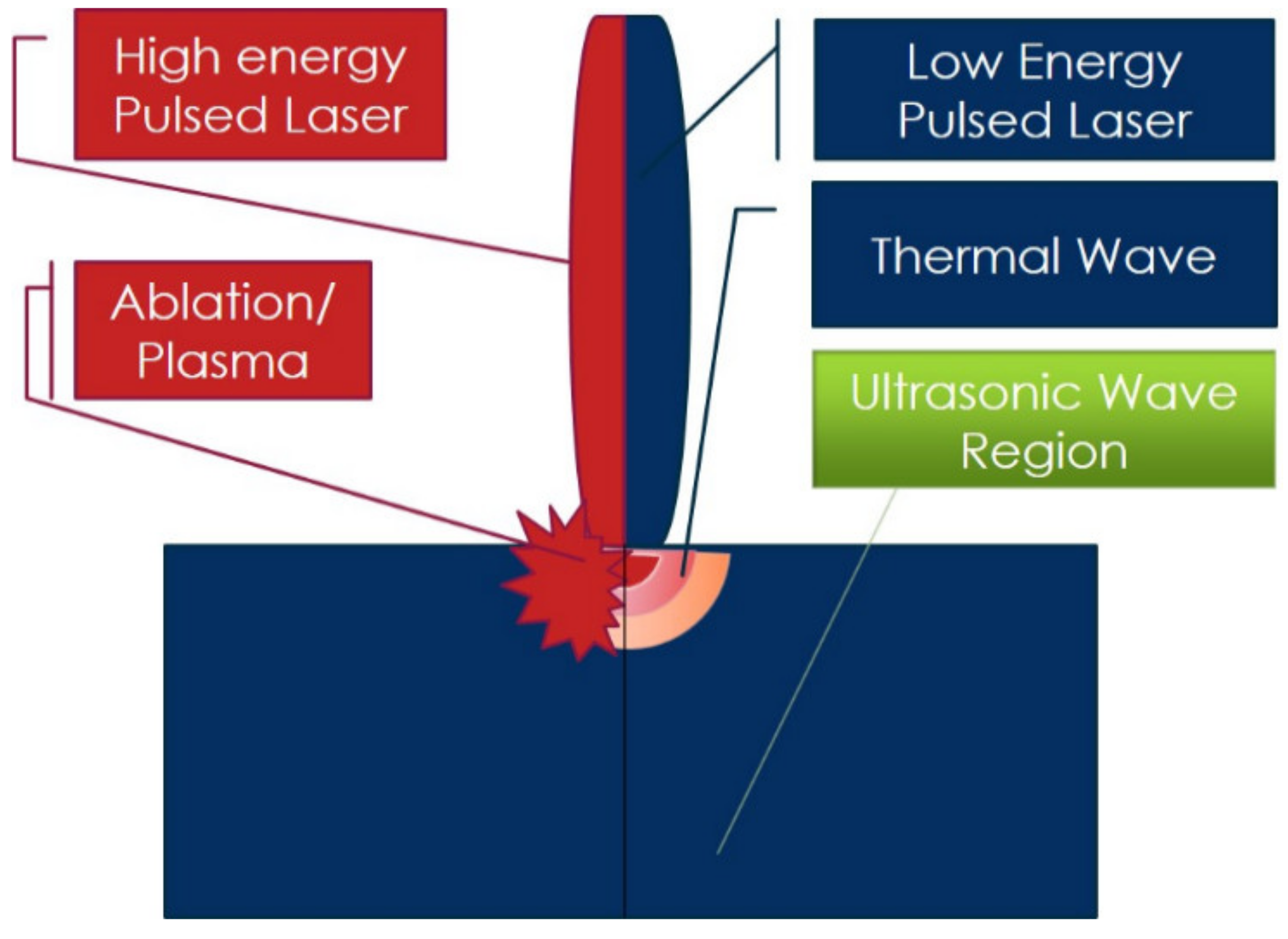
2.1. System Mechanism
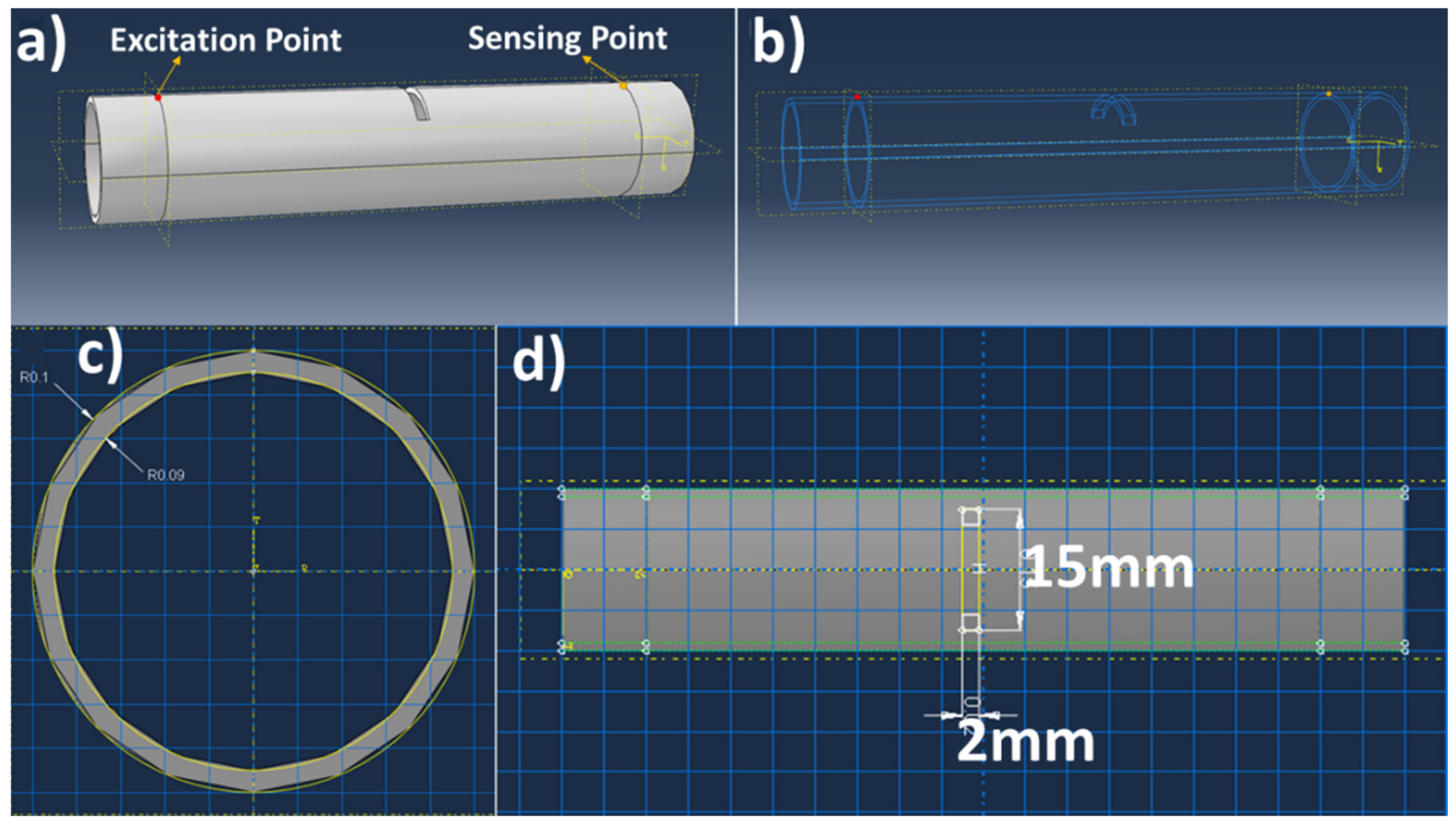
2.2. Simulation Setup
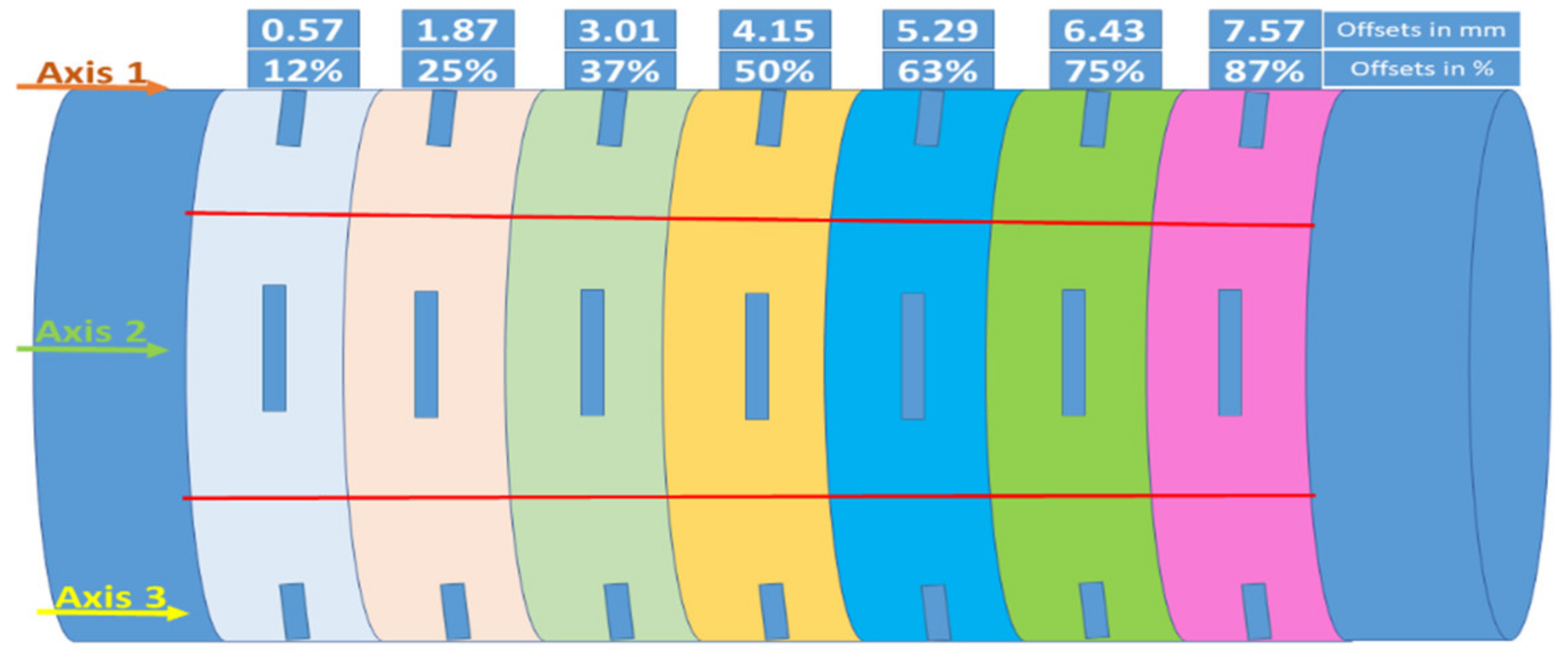
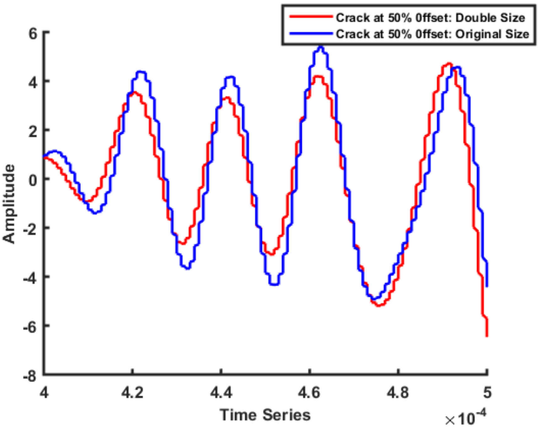
2.2.1. Simulation Geometry Variations
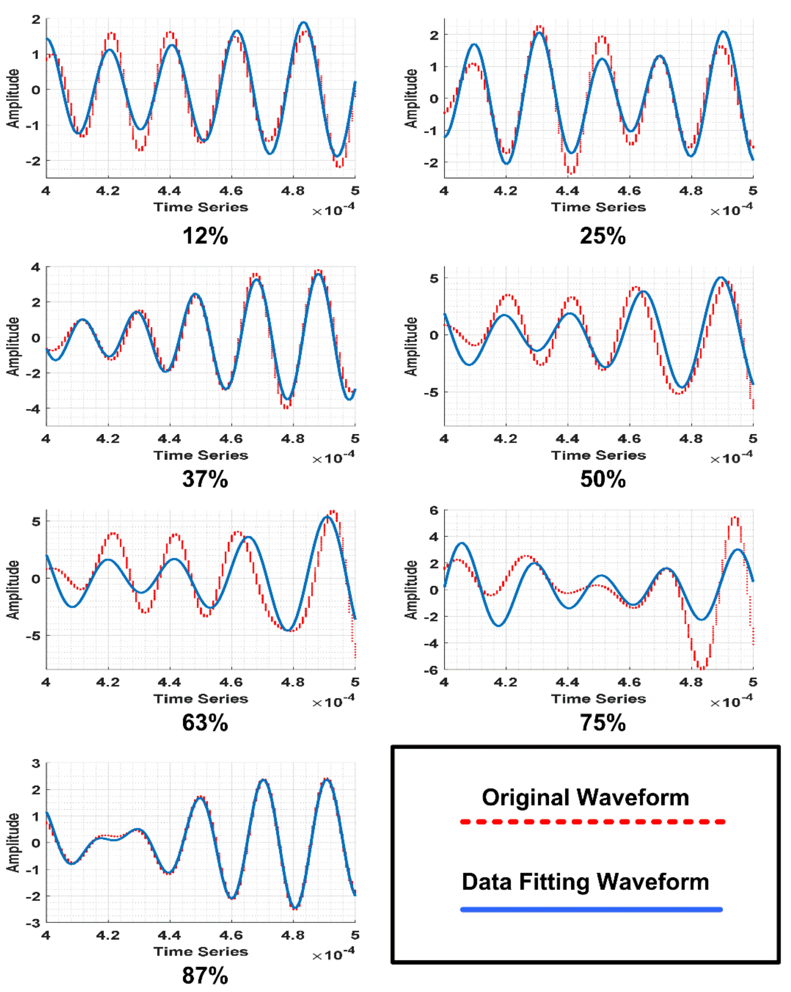
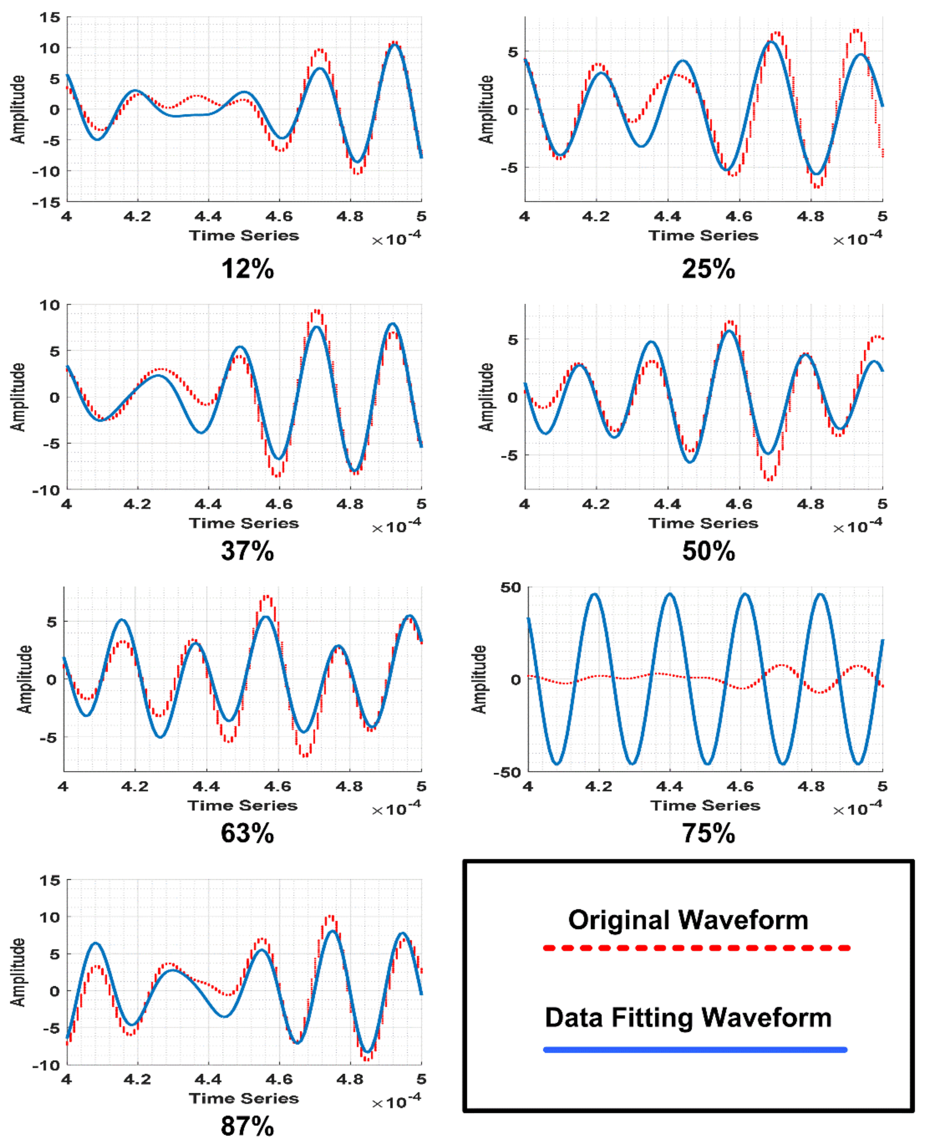
2.2.2. Different Crack Sizes
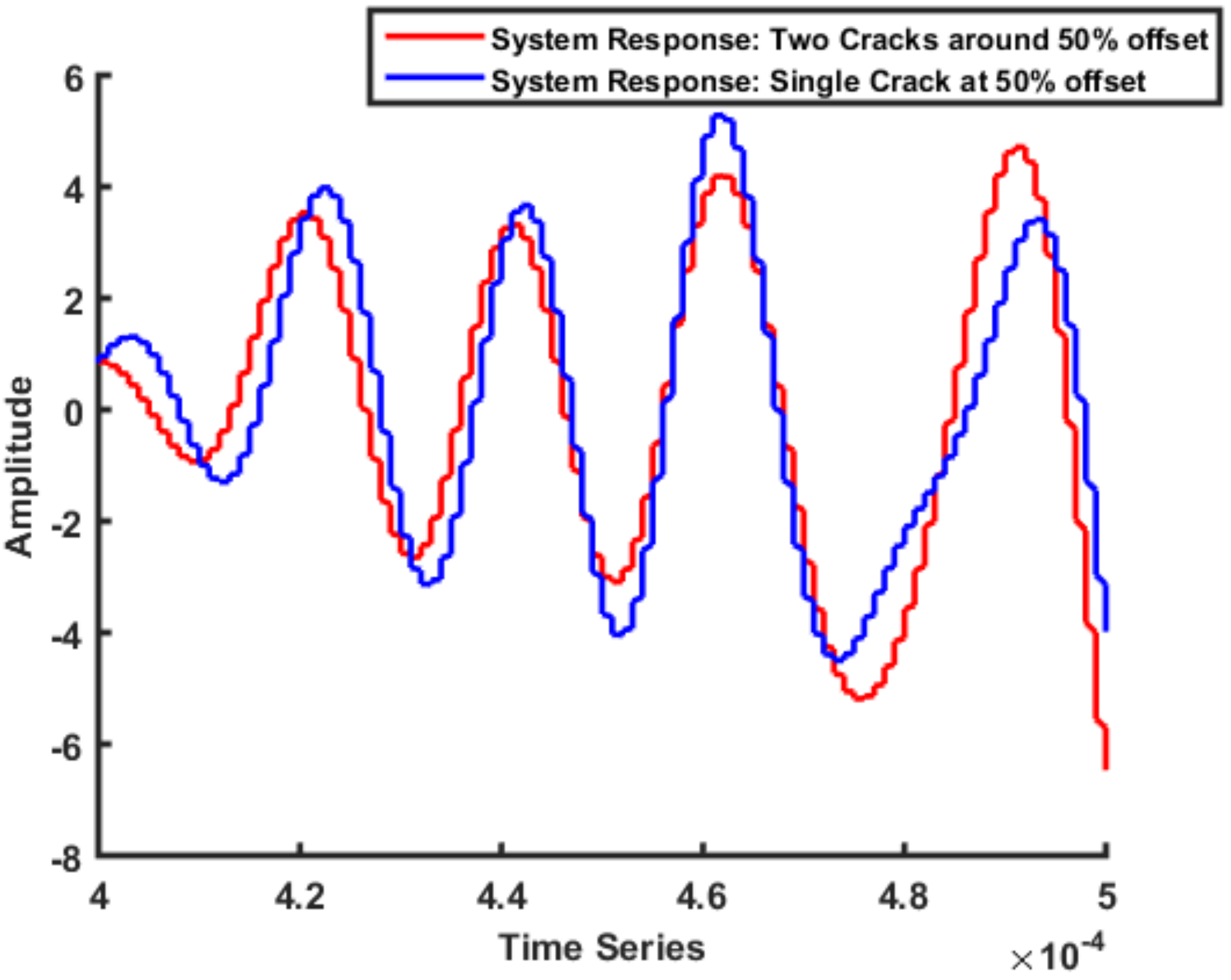
2.2.3. Multiple Cracks
2.3. Data Acquisition and Preprocessing
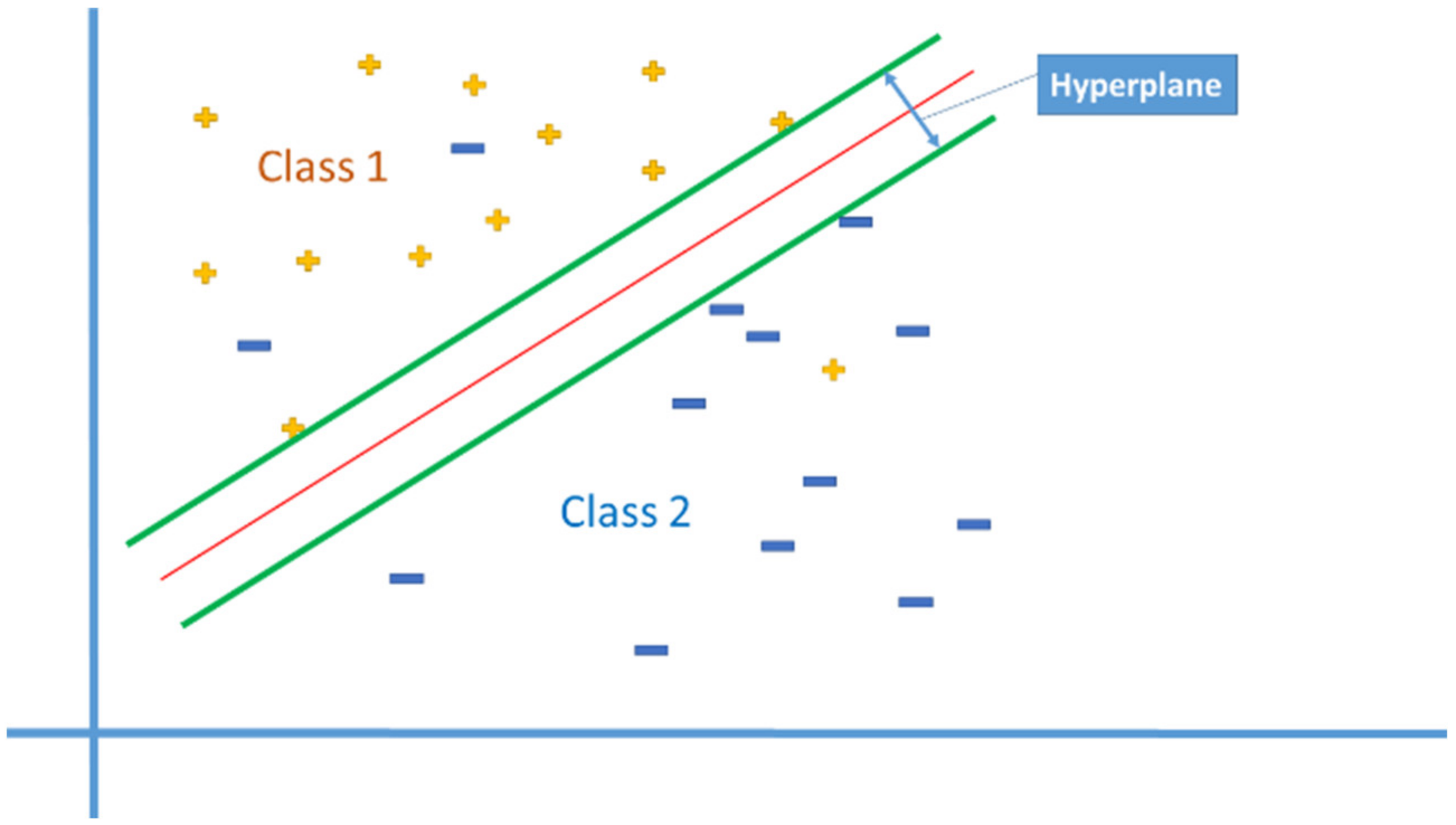
Classification
3. Results and Discussions
4. Conclusions
Author Contributions
Funding
Institutional Review Board Statement
Informed Consent Statement
Conflicts of Interest
References
- Hou, B.; Li, X.; Ma, X.; Du, C.; Zhang, D.; Zheng, M.; Xu, W.; Lu, D.; Ma, F. The cost of corrosion in China. npj Mater. Degrad. 2017, 1, 1–10. [Google Scholar] [CrossRef]
- Flint, G.; Packirisamy, S.J. Purity of food cooked in stainless steel utensils. Food Addit. Contam. 1997, 14, 115–126. [Google Scholar] [CrossRef]
- Liu, Q.; Zhu, Y.; Yuan, X.; Zhang, J.; Wu, R.; Dou, Q.; Liu, S. Internet of Things Health Detection System in Steel Structure Construction Management. IEEE Access 2020, 8, 147162–147172. [Google Scholar] [CrossRef]
- Lo, K.H.; Shek, C.H.; Lai, J.K.L. Recent developments in stainless steels. Mater. Sci. Eng. R Rep. 2009, 65, 39–104. [Google Scholar] [CrossRef]
- Baddoo, N.R. Stainless steel in construction: A review of research, applications, challenges and opportunities. J. Constr. Steel Res. 2008, 64, 1199–1206. [Google Scholar] [CrossRef]
- Oluwasola, E.A.; Hainin, M.R.; Aziz, M.M.A. Characteristics and utilization of steel slag in road construction. Jurnal Teknologi 2014, 70, 117–123. [Google Scholar] [CrossRef] [Green Version]
- Kerouedan, J.; Queffelec, P.; Talbot, P.; Quendo, C.; De Blasi, S.; Le Brun, A. Detection of micro-cracks on metal surfaces using near-field microwave dual-behavior resonator filters. Meas. Sci. Technol. 2008, 19, 105701. [Google Scholar] [CrossRef]
- Lankford, J.; Kusenberger, F.J. Initiation of fatigue cracks in 4340 steel. Metall. Trans. 1973, 4, 553–559. [Google Scholar] [CrossRef]
- Liu, S.; Chai, K.; Zhang, C.; Jin, L.; Yang, Q.J. Electromagnetic Acoustic Detection of Steel Plate Defects Based on High-Energy Pulse Excitation. Appl. Sci. 2020, 10, 5534. [Google Scholar] [CrossRef]
- Otegui, J.; Kerr, H.; Burns, D.; Mohaupt, U.J. Fatigue crack initiation from defects at weld toes in steel. Int. J. Press. Vessel. Pip. 1989, 38, 385–417. [Google Scholar] [CrossRef]
- Rajan, K.; Narasimhan, K.J. An investigation of the development of defects during flow forming of high strength thin wall steel tubes. Pract. Fail. Anal. 2001, 1, 69–76. [Google Scholar] [CrossRef]
- Soukup, D.; Huber-Mörk, R. Convolutional neural networks for steel surface defect detection from photometric stereo images. In International Symposium on Visual Computing; Springer: Cham, Switzerland, 2014; pp. 668–677. [Google Scholar]
- ASCE. 2021 Report Card for America’s Infrastructure. American Society of Civil Engineers: Reston, VA, USA, 2021. Available online: https://infrastructurereportcard.org/wp-content/uploads/2020/12/2021-IRC-Executive-Summary-1.pdf (accessed on 25 June 2021).
- Geng, J.; Sun, Q.; Zhang, Y.; Cao, L.; Zhang, W. Studying the dynamic damage failure of concrete based on acoustic emission. Constr. Build. Mater. 2017, 149, 9–16. [Google Scholar] [CrossRef]
- Gholizadeh, S. A review of non-destructive testing methods of composite materials. Procedia Struct. Integr. 2016, 1, 50–57. [Google Scholar] [CrossRef] [Green Version]
- Shah, S.G.; Kishen, J.C. Use of acoustic emissions in flexural fatigue crack growth studies on concrete. Eng. Fract. Mech. 2012, 87, 36–47. [Google Scholar] [CrossRef]
- Ramani, V.; Kuang, K.S.C. Monitoring chloride ingress in concrete using an imaging probe sensor with sacrificial metal foil. Autom. Constr. 2020, 117, 103260. [Google Scholar] [CrossRef]
- Schlichting, J.; Maierhofer, C.; Kreutzbruck, M.; International, E. Crack sizing by laser excited thermography. NDT E Int. 2012, 45, 133–140. [Google Scholar] [CrossRef]
- Xu, Y.; Li, S.; Zhang, D.; Jin, Y.; Zhang, F.; Li, N.; Li, H. Identification framework for cracks on a steel structure surface by a restricted Boltzmann machines algorithm based on consumer-grade camera images. Struct. Control. Health Monit. 2018, 25, e2075. [Google Scholar] [CrossRef]
- Wang, N.; Zhao, Q.; Li, S.; Zhao, X.; Zhao, P. Damage classification for masonry historic structures using convolutional neural networks based on still images. Comput. Aided Civ. Infrastruct. Eng. 2018, 33, 1073–1089. [Google Scholar] [CrossRef]
- Carden, E.P.; Fanning, P. Vibration based condition monitoring: A review. Struct. Health Monit. 2004, 3, 355–377. [Google Scholar] [CrossRef]
- Khan, A.; Stanbridge, A.B.; Ewins, D.J. Detecting damage in vibrating structures with a scanning LDV. Opt. Lasers Eng. 1999, 32, 583–592. [Google Scholar] [CrossRef]
- Walker, S.V.; Kim, J.-Y.; Qu, J.; Jacobs, L.J. Fatigue damage evaluation in A36 steel using nonlinear Rayleigh surface waves. NDT E Int. 2012, 48, 10–15. [Google Scholar] [CrossRef]
- Sagar, S.P.; Parida, N.; Das, S.; Dobmann, G.; Bhattacharya, D.K. Magnetic Barkhausen emission to evaluate fatigue damage in a low carbon structural steel. Int. J. Fatigue 2005, 27, 317–322. [Google Scholar] [CrossRef]
- Chang, Y.; Jiao, J.; Liu, X.; Li, G.; He, C.; Wu, B. Nondestructive evaluation of fatigue in ferromagnetic material using magnetic frequency mixing technology. NDT E Int. 2020, 111, 102209. [Google Scholar] [CrossRef]
- Man, J.; Vystavěl, T.; Weidner, A.; Kuběna, I.; Petrenec, M.; Kruml, T.; Polák, J. Study of cyclic strain localization and fatigue crack initiation using FIB technique. Int. J. Fatigue 2012, 39, 44–53. [Google Scholar] [CrossRef]
- Ding, X.; Li, W.; Xiong, J.; Shen, Y.; Huang, W. A flexible laser ultrasound transducer for Lamb wave based structural health monitoring. Smart Mater. Struct. 2020, 29, 075006. [Google Scholar] [CrossRef]
- Kim, Y.-M.; Han, G.; Kim, H.; Oh, T.-M.; Kim, J.-S.; Kwon, T.-H. An Integrated Approach to Real-Time Acoustic Emission Damage Source Localization in Piled Raft Foundations. Appl. Sci. 2020, 10, 8727. [Google Scholar] [CrossRef]
- Naeimi, M.; Li, Z.; Qian, Z.; Zhou, Y.; Wu, J.; Petrov, R.H.; Sietsma, J.; Dollevoet, R. Reconstruction of the rolling contact fatigue cracks in rails using X-ray computed tomography. NDT E Int. 2017, 92, 199–212. [Google Scholar] [CrossRef]
- Wang, R.; Liu, F.; Hou, F.; Jiang, W.; Hou, Q.; Yu, L. A non-contact fault diagnosis method for rolling bearings based on acoustic imaging and convolutional neural networks. IEEE Access 2020, 8, 132761–132774. [Google Scholar] [CrossRef]
- Guldur, B.; Yan, Y.; Hajjar, J.F. Condition assessment of bridges using terrestrial laser scanners. In Structures Congress; American Society of Civil Engineers: Reston, VA, USA, 2015; pp. 355–366. [Google Scholar]
- Rucka, M.; Zima, B.; Kędra, R. Application of guided wave propagation in diagnostics of steel bridge components. Arch. Civ. Eng. 2014, 60, 493–516. [Google Scholar] [CrossRef] [Green Version]
- Park, D.-G.; Angani, C.S.; Rao, B.; Vértesy, G.; Lee, D.-H.; Kim, K.-H. Detection of the subsurface cracks in a stainless steel plate using pulsed eddy current. J. Nondestruct. Eval. 2013, 32, 350–353. [Google Scholar] [CrossRef]
- Knitter-Piątkowska, A.; Dobrzycki, A. Application of Wavelet Transform to Damage Identification in the Steel Structure Elements. Appl. Sci. 2020, 10, 8198. [Google Scholar] [CrossRef]
- Tang, S.; Wang, R.; Han, J. Acoustic Focusing Imaging Characteristics Based on Double Negative Locally Resonant Phononic Crystal. IEEE Access 2019, 7, 112598–112604. [Google Scholar] [CrossRef]
- Billeh, Y.N.; Liu, M.; Buma, T. Spectroscopic photoacoustic microscopy using a photonic crystal fiber supercontinuum source. Opt. Express 2010, 18, 18519–18524. [Google Scholar] [CrossRef] [PubMed]
- Granchi, S.; Vannacci, E.; Miris, L.; Onofri, L.; Zingoni, D.; Biagi, E. Spectral Analysis of Ultrasonic and Photo Acoustic Signals Generated by a Prototypal Fiber Microprobe for Media Characterization. Sens. Imaging 2020, 21, 1–13. [Google Scholar] [CrossRef]
- Minonzio, J.-G.; Cataldo, B.; Olivares, R.; Ramiandrisoa, D.; Soto, R.; Crawford, B.; De Albuquerque, V.H.C.; Munoz, R. Automatic Classifying of Patients with Non-Traumatic Fractures Based on Ultrasonic Guided Wave Spectrum Image Using a Dynamic Support Vector Machine. IEEE Access 2020, 8, 194752–194764. [Google Scholar] [CrossRef]
- Fitzpatrick, A.; Singhvi, A.; Arbabian, A. An Airborne Sonar System for Underwater Remote Sensing and Imaging. IEEE Access 2020, 8, 189945–189959. [Google Scholar] [CrossRef]
- Liu, P.; Sohn, H. Numerical simulation of damage detection using laser-generated ultrasound. Ultrasonics 2016, 69, 248–258. [Google Scholar] [CrossRef]
- Kamran, M.A.; Jeong, M.Y.; Mannan, M. Optimal hemodynamic response model for functional near-infrared spectroscopy. Front. Behav. Neurosci. 2015, 9, 151. [Google Scholar] [CrossRef] [Green Version]
- Gong, L.; Yu, X.; Wang, J. Curve-Localizability-SVM Active Localization Research for Mobile Robots in Outdoor Environments. Appl. Sci. 2021, 11, 4362. [Google Scholar] [CrossRef]
- Wang, S.; Echeverry, J.; Trevisi, L.; Prather, K.; Xiang, L.; Liu, Y. Ultrahigh resolution pulsed laser-induced photoacoustic detection of multi-scale damage in CFRP composites. Appl. Sci. 2020, 10, 2106. [Google Scholar] [CrossRef] [Green Version]
- Li, X.; Shui, G.; Zhao, Y.; Wang, Y.-S. Propagation of Non-Linear Lamb Waves in Adhesive Joint with Micro-Cracks Distributing Randomly. Appl. Sci. 2020, 10, 741. [Google Scholar] [CrossRef] [Green Version]
- Kazys, R.J.; Mazeika, L.; Sestoke, J. Development of ultrasonic techniques for measurement of spatially non-uniform elastic properties of thin plates by means of a guided sub-sonic A0 mode. Appl. Sci. 2020, 10, 3299. [Google Scholar] [CrossRef]
- Park, S.-H.; Kim, J.; Song, D.-G.; Choi, S.; Jhang, K.-Y. Measurement of Absolute Acoustic Nonlinearity Parameter Using Laser-Ultrasonic Detection. Appl. Sci. 2021, 11, 4175. [Google Scholar] [CrossRef]
- Guan, L.; Zou, M.; Wan, X.; Li, Y. Nonlinear Lamb wave micro-crack direction identification in plates with mixed-frequency technique. Appl. Sci. 2020, 10, 2135. [Google Scholar] [CrossRef] [Green Version]


| Property | Value |
|---|---|
| Density | 8207 kg/m3 |
| Poisson’s Ratio | 0.33 |
| Young’s Modulus | 129 GPa |
| A | 1 | O | 12 | S |
| 25 | ||||
| 37 | ||||
| 2 | 50 | |||
| 62 | M | |||
| 3 | 75 | |||
| 87 |
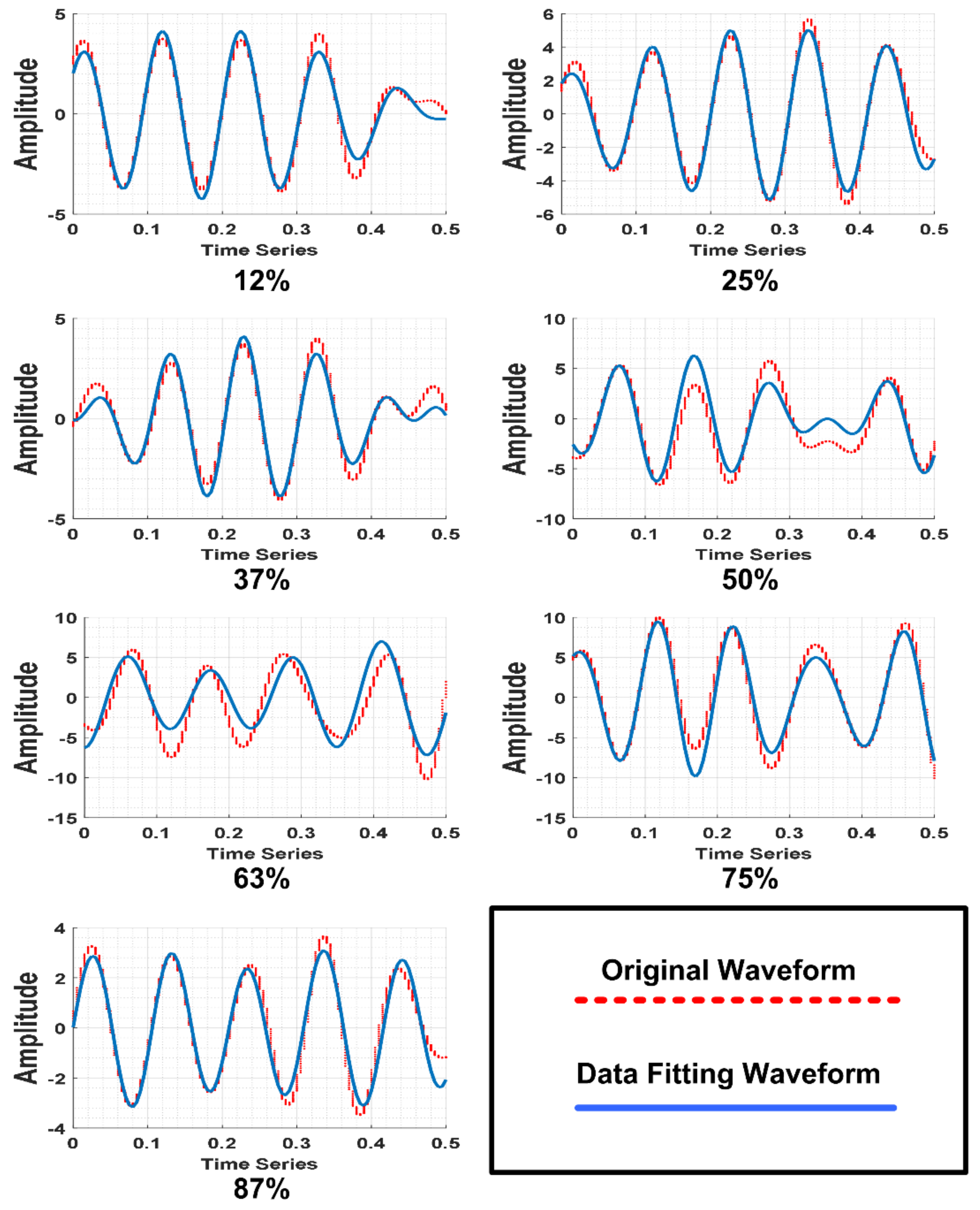
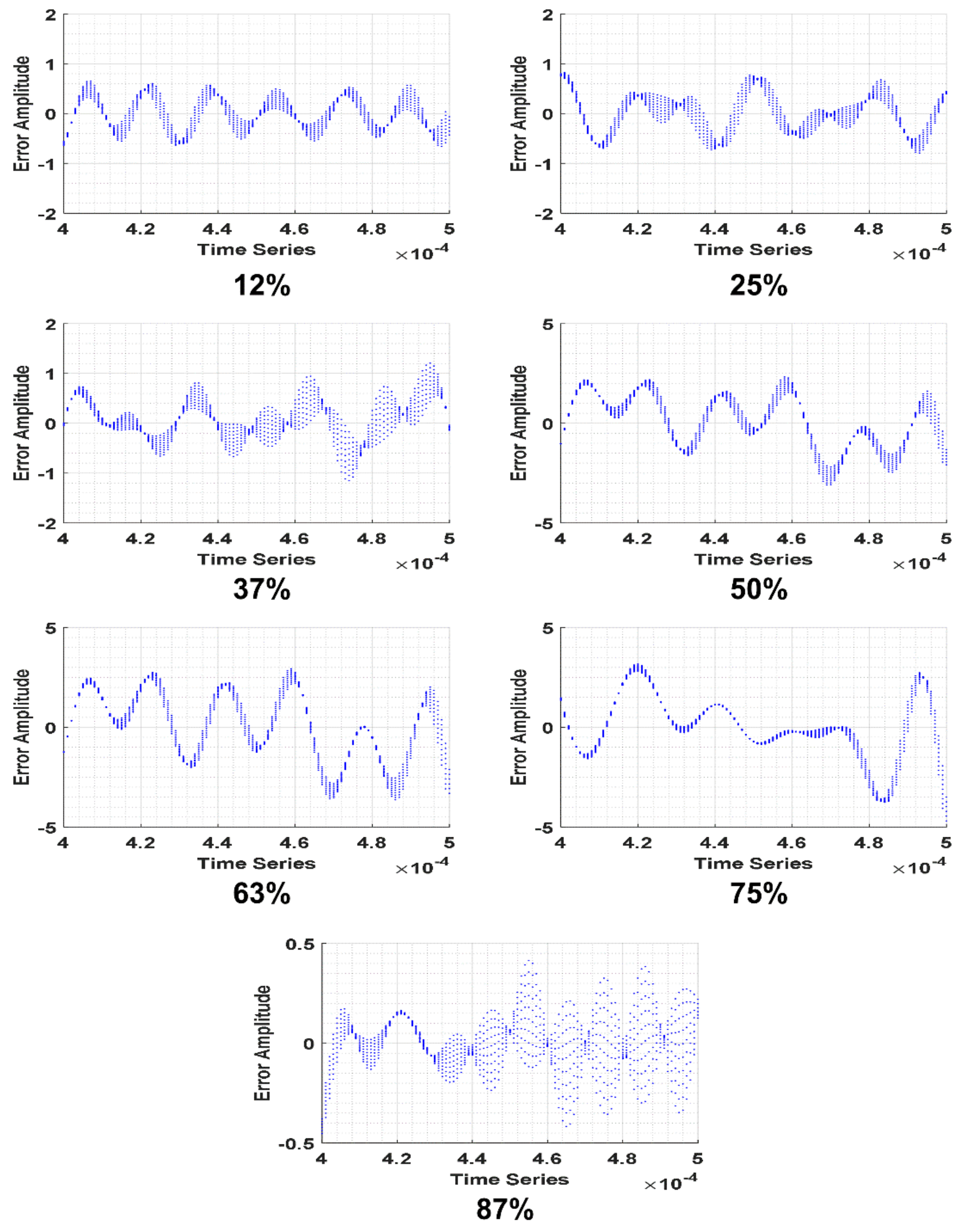
| Crack (Axis 1) | Amplitude 1 | Frequency 1 KHz | Phase 1 | Amplitude 2 | Frequency 2 KHz | Phase 2 | RMSE |
|---|---|---|---|---|---|---|---|
| 12% | 1.51 | 298.40 | 8.13 | 0.40 | 247.90 | 1.32 | 0.32 |
| 25% | 1.58 | 313.80 | −1.53 | 0.54 | 220.70 | 12.95 | 0.27 |
| 37% | 2.31 | 327.70 | −7.57 | 1.30 | 285.60 | −18.40 | 0.40 |
| 50% | 3.28 | 262.10 | −7.47 | 1.88 | 216.60 | −9.95 | 1.32 |
| 67% | 3.81 | 254.40 | −4.32 | 2.53 | 221.10 | −11.99 | 1.68 |
| 75% | 69.22 | 254.50 | −28.17 | 70.27 | 255.50 | −0.34 | 1.24 |
| 87% | 1.16 | 331.30 | −9.97 | 1.30 | 278.60 | −9.77 | 0.13 |
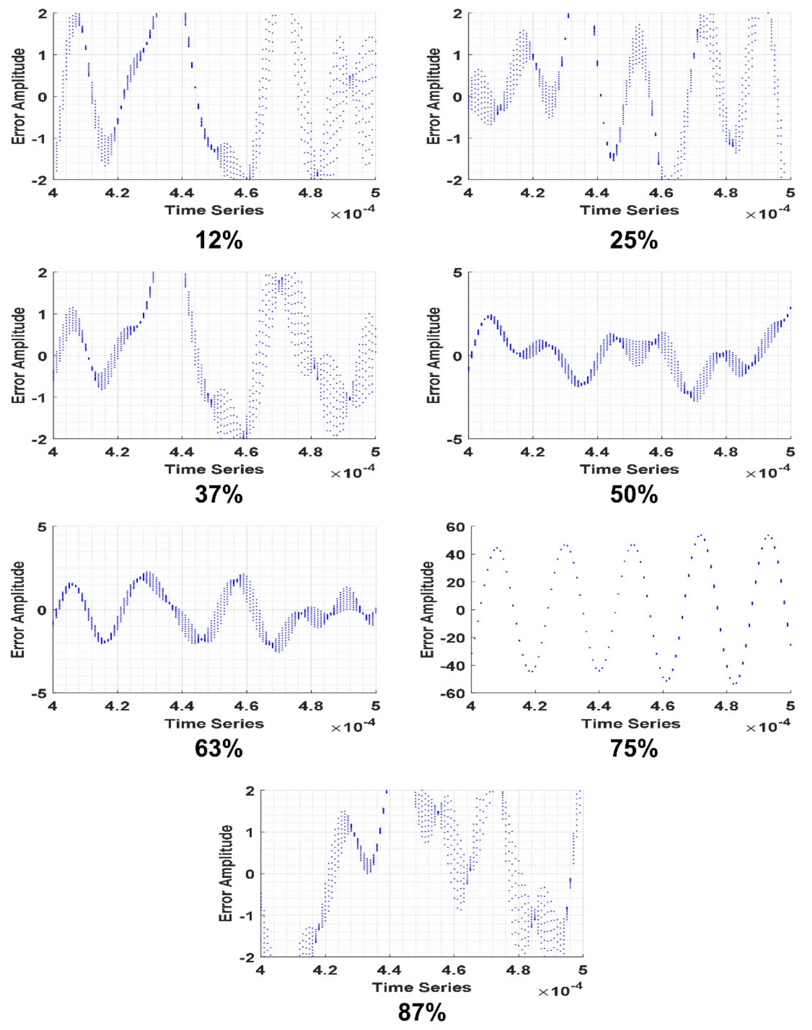
| Crack (Axis 2) | Amplitude 1 | Frequency 1 KHz | Phase 1 | Amplitude 2 | Frequency 2 KHz | Phase 2 | RMSE |
|---|---|---|---|---|---|---|---|
| 12% | 37.39 | 295.8 | −17.3 | 36.42 | 300.8 | 2.785 | 1.47 |
| 25% | 4.47 | 262.00 | −1.92 | 1.41 | 193.70 | −1.11 | 1.52 |
| 37% | 5.02 | 273.90 | −7.60 | 3.06 | 321.30 | −5.45 | 1.37 |
| 50% | 4.29 | 303.40 | 7.49 | 1.54 | 221.50 | 13.11 | 1.17 |
| 63% | 4.21 | 314.00 | 2.70 | 1.31 | 146.70 | −8.49 | 1.19 |
| 75% | 2301.00 | 295.60 | −16.93 | 2301.00 | 295.60 | 5.04 | 1.53 |
| 87% | 5.47 | 293.20 | 7.05 | 2.91 | 357.80 | 7.27 | 1.80 |
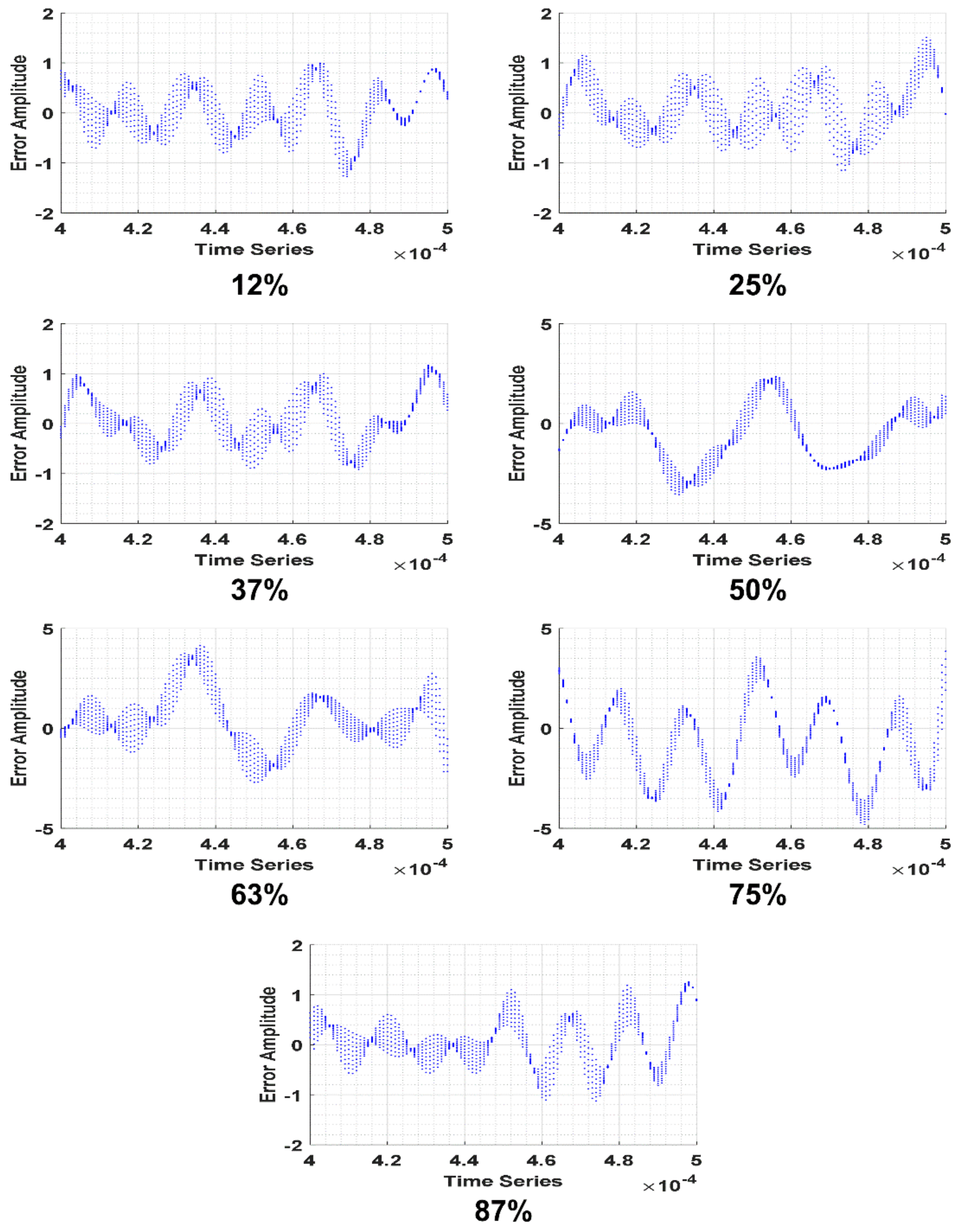
| Crack (Axis 3) | Amplitude 1 | Frequency 1 KHz | Phase 1 | Amplitude 2 | Frequency 2 KHz | Phase 2 | RMSE |
|---|---|---|---|---|---|---|---|
| 12% | 1.94 | 323.90 | −4.05 | 2.33 | 275.80 | −8.29 | 0.47 |
| 25% | 1.73 | 329.50 | −7.25 | 3.41 | 284.60 | −11.90 | 0.49 |
| 37% | 2.02 | 282.90 | 13.71 | 2.08 | 350.10 | 15.17 | 0.49 |
| 50% | 3.22 | 259.70 | −4.42 | 3.20 | 335.10 | −11.60 | 1.47 |
| 63% | 5.31 | 262.80 | −5.89 | 1.90 | 207.30 | −10.00 | 2.03 |
| 75% | 2.49 | 361.60 | −20.10 | 7.42 | 279.50 | −9.80 | 1.41 |
| 87% | 2.76 | 305.00 | 3.53 | 0.40 | 192.30 | 0.28 | 0.47 |
Publisher’s Note: MDPI stays neutral with regard to jurisdictional claims in published maps and institutional affiliations. |
© 2021 by the authors. Licensee MDPI, Basel, Switzerland. This article is an open access article distributed under the terms and conditions of the Creative Commons Attribution (CC BY) license (https://creativecommons.org/licenses/by/4.0/).
Share and Cite
Akbar, A.; Kamran, M.A.; Kim, J.; Jeong, M.Y. Mathematical Modeling and Computer-Aided Simulation of the Acoustic Response for Cracked Steel Specimens. Appl. Sci. 2021, 11, 7699. https://doi.org/10.3390/app11167699
Akbar A, Kamran MA, Kim J, Jeong MY. Mathematical Modeling and Computer-Aided Simulation of the Acoustic Response for Cracked Steel Specimens. Applied Sciences. 2021; 11(16):7699. https://doi.org/10.3390/app11167699
Chicago/Turabian StyleAkbar, Arbab, Muhammad Ahmad Kamran, Jeesu Kim, and Myung Yung Jeong. 2021. "Mathematical Modeling and Computer-Aided Simulation of the Acoustic Response for Cracked Steel Specimens" Applied Sciences 11, no. 16: 7699. https://doi.org/10.3390/app11167699