Abstract
The purpose of this paper is to design a lizard-inspired robot driven by a single actuator. Lizard-inspired robots in previous studies had the issue of slippage of their supporting legs. To overcome this issue, a lizard-inspired robot consisting of a four-bar linkage mechanism was designed. The purpose of this paper was achieved through three processes. The first process was kinematic analysis, where the turning angle and stride length of the robot were analyzed. The kinematic analysis results were verified via numerical simulations. The second process was the design and fabrication of the robot. For the robot’s design, both a shuffle-walking method utilizing a claw-shaped leg mechanism and a sliding-rod mechanism for equipping the actuator on the robot’s own coordinates were designed. The third process was experimental verification. The first experimental result was that the claw-shaped leg mechanism was capable of generating an 85.26 N difference in the static frictional force in the longitudinal direction. The other three experimental results were that the robot was capable of driving with 3.51%, 3.16%, and 3.53% error compared to the kinematic analyses, respectively.
1. Introduction
Legged robots are always the most popular choice for robotics researchers due to their benefits over traditional wheeled robots or those that follow automated stages in applications such as mobility over irregular terrain [1,2,3]. Bartsch et al. built the “Space-Climber 1”, which is a bio-inspired, six-legged, and vibrancy-effective robot. This robot was planned for use in extraterrestrial surface investigation, especially for portability in lunar pits [4]. Estremera et al. described the improvement of a hexapod robot, “SILO-6”, using crab and turning gaits. Their robot was designed to move across a characteristic landscape containing uneven ground, and it can be used for humanitarian demining [5]. Moro et al. proposed an approach of directly mapping a range of horse gaits to a quadruped robot with the intention of generating a more realistic locomotion gait [6]. Ref. [6] also used kinematic motion primitives to generate stable and valid walking, trotting, and galloping gaits in a compliant quadruped robot. Refs. [4,5,6] developed robots that were generally effective in mimicking the gait cycles of their biological counterparts; however, they suffered from a high payload-to-machine-load ratio and high energy consumption.
Several approaches to developing energy-efficient walking machines have been reported. Ref. [7] developed a set of rules to improve energy efficiency in statically-stable walking robots by comparing two-legged mammal and insect configurations on a hexapod robotic platform.Ref. [8] applied the minimization criterion to optimize energy efficiency in a hexapod robot with respect to each half of a locomotion cycle, especially walking on uneven terrain. Ref. [9] discussed two significant energy-efficient approaches toward determining optimal foot forces and joint torques for a six-legged robot.
In order to solve this problem, multi-legged robots that can be driven with a small number of actuators have been studied. Jansen [10], a Dutch kinetic artist, proposed an unconventional closed kinematic-chain-based approach that requires actuation at only a single leg by mapping internal cyclic motion into elliptical motion. Various aspects of the Jansen mechanism have been studied by a number of researchers. In [11,12], the authors proposed an extension of Theo Jansen’s mechanism by introducing an additional up–down motion in the linkage center in order to realize new gait cycles, with approximately 10 times the height of the original, for climbing over obstacles. A vector loop and simple geometric methods were used in conjunction with software tools, such as ProEngineer and SAM, to analyze the forward kinematics of Theo Jansen’s mechanism in [13]. An attempt to optimize the leg geometry of Theo Jansen’s mechanism using the genetic algorithm was presented in [14]. This work explored the stability limits and tractive abilities while validating the kinematic and kinetic models through experiments with hardware prototypes. In [15], a preliminary dynamic analysis was performed using the superposition method with the intention of optimizing Theo Jansen’s mechanism. Ref. [16] developed an eight-legged walking robot that consisted of Theo Jansen’s mechanism and experimentally demonstrated its effectiveness in both flat and stair-climbing environments. In [17], we presented a dynamic analysis of a four-legged Theo Jansen link mechanism using the projection method, which resulted in constraint force and an equivalent Lagrange equation of motion. In [18,19], the design of a novel reconfigurable Theo Jansen linkage was put forward and validated. This design produced a wide variety of gait cycles, opening new possibilities for innovative applications. The suggested mechanism switched from a pin-jointed Grübler kinematic chain to a five-degree-of-freedom mechanism with slider joints during the reconfiguration process. An original design approach was presented in [20] to develop a trajectory generator that realized a set of stable walking gaits, gait synchronization, and a transition for a reconfigurable Jansen platform.
Another example is 1STAR, a six-legged robot capable of being driven with one degree of freedom [21,22,23]. This robot consists of a rectangular body with six legs attached to both the vertex of the rectangular body and its long sides. The movements of the six legs are synchronized by gears, and the difference in the elasticity of the legs—thanks to the effects of torsion springs—is utilized to achieve forward and turning locomotion. STAR, which was developed by the same team, is a sprawl-tuned hexapod robot driven by three actuators: Two actuators work to drive the left and right legs, and the third actuator is used for the sprawl angle [24,25,26]. SAW is a robot that can be driven by a single actuator and can move forward by generating a wave-like motion [27,28]. SAW has a spine that constrains the links from moving around it, producing an advancing wave-like motion. SAW is also able to drive between two flexible surfaces. HIbot is a single-actuated mobile crawling robot inspired by hexapod insects [29]. It consists of six wheeled-leg mechanisms with four spokes and two bodies connected by passive joints. The six wheeled-leg mechanisms are appropriately synchronized by a belt, and it has been shown to be able to propel itself on stairs and uneven environments.
Another example of an approach to multi-legged robots driven with a lower number of actuators is the bio-inspired approach. Ref. [30] categorized the morphologies of multi-legged robots into the mammal type, called “M-type,” and the insect type, called “I-type,” and concluded that the I-type is more efficient than the M-type when using a leg mechanism for a walking robot. A lizard possesses the I-type morphology. It improves its walking efficiency through the flexion movement of the trunk instead of through leg locomotion, especially when running quickly. This characteristic enabled us to decrease the number of actuators, and may even lead to a multi-legged robot that is driven by a single actuator, which will help in addressing the issue of the energy efficiency of multi-legged robots. A team at the College of Industrial Technology found that a lizard mainly walks by only twisting its waist [31]. The same team analyzed the kinematics and then developed and demonstrated a lizard-type robot [32,33]. In our previous study, the dynamics of a lizard-type robot were analyzed [34], and a robot capable of walking with only a single actuator was developed [35]. The robot in [31,32,33,34,35] had the morphology depicted in Figure 1. This morphology consists of two facing triangles whose vertices are secured by an active pin joint. The vertices other than the active joint work as the legs. The active joints are swung sinusoidally, and the robot walks forward.
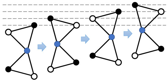
Figure 1.
The kinematic model used in previous studies [31,32,33,34,35]. If the support legs (depicted by black circles) are completely fixed, then the waist (depicted by blue circles) can only exist at an equal point from each of the support legs, and is therefore constrained to one of the two distant points. Thus, when the angle of the waist is moved continuously, the positions of the support legs also change continuously (i.e., they slip).
Although related studies have shown interesting results, including experiments, these robots cannot walk unless the support legs slip, or they require additional actuators to change their propulsive direction. For example, the Theo Jansen mechanism similarly requires its legs to slip in order to walk. In [17,18,19], kinematic and dynamic analyses were addressed, and the velocity of the leg was shown to vary non-linearly. Hence, when driven synchronously in a certain phase, the legs of the Theo Jansen walking robot have different speeds (i.e., the support legs slip). In [36], the trajectory generation method was proposed to maintain a constant leg velocity. However, to apply this trajectory generation method to a multi-legged robot, it is necessary to install an actuator on each leg. Thus, it cannot be driven by a single actuator alone. Meanwhile, 1STAR also requires the legs to slip in order to walk because the legs, which are equipped on the rectangular sides, are forced to slip geometrically for continuous leg driving. In fact, their team designed their robot based on a dynamic analysis that included the coefficient of friction with the ground. However, the coefficient of friction with the ground varies from place to place. Hence, a case-by-case analysis is required for a proper analysis of the locomotion of the robot. SAWs and HIbots are also only mechanically capable of moving forward or backward. Therefore, they require an additional actuator to change the propulsive direction.
Similarly, in a lizard-like robot with the morphology shown in Figure 1, if the support legs depicted in black circles are completely fixed, then the waist (depicted in blue circles) can only exist at an equal point from each of the support legs, which are therefore constrained to one of the two distant points. Thus, when the angle of the waist is moved continuously, the position of the support legs also changes continuously (i.e., they slip). These issues are disadvantages, and they require a complex dynamic analysis, including an analysis of the friction coefficients with the ground, to know the kinematics of the robot. More specifically, it is difficult to achieve accurate motion control because the control system is also required to consider unknown toe slippage.
The purpose of this paper was to implement a lizard-inspired robot that is capable of being driven by a single actuator. Our proposed lizard-inspired robot overcomes these disadvantages because our robot possesses a morphology consisting of a four-bar linkage mechanism, as depicted in Figure 2. The morphology of the four-bar linkage mechanism is able to regard the fixed link as the support leg and can be driven without the slipping of the support leg. By switching the fixed links of the support legs appropriately, we realized a robot that is theoretically capable of walking without its support legs slipping. This is the biggest difference between our robot and those of the related research, and it is our main novelty. This provides the robot with appropriate walking in which its support legs do not slip. It also allows the robot to formulate proper kinematic characteristics via kinematic analyses, which are much simpler than dynamic analyses. The robot moves forward by setting the fixed link of a four-bar linkage mechanism as support legs, and then switching them. The purpose of this paper was achieved through the following three processes.
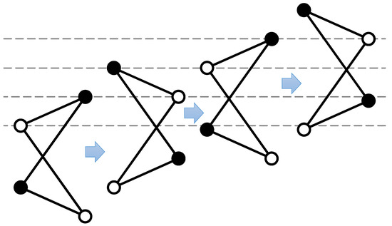
Figure 2.
A kinematic model of the lizard-type robot proposed in this study. When the front link is driven during walking, the distance of the supporting leg, depicted in the black circle, does not change. Therefore, our proposed model can drive the supporting legs without slipping.
The first process was a kinematic analysis. In this paper, a biased sinusoidal input angle function was adopted as the input for the system. The two ideas for the kinematic analysis were to define our own robot model and to formulate the kinematic characteristics based on the period of the input angle function. In particular, the first idea was to set a “robot coordinate” at the center of the front link. The robot coordinate allowed us to represent symmetrically important states, such as a turning angle and related angles between each link. In the second idea, the kinematics were characterized with respect to each half-period of the input angle function. Since the robot consists of a four-bar linkage mechanism, the same kinematic characteristics are maintained unless the support legs are switched. Hence, formulating the kinematic characteristics of the robot at the switching of the support legs can adequately represent the kinematic characteristics of the robot. In this paper, we formulated a turning angle and a stride length. These two characteristics are important for understanding the locomotion of the robot. In the turning locomotion analysis, it was proven that the robot turns with constant curvature by adding a constant bias onto the input angle. In the stride-length analysis, it was proven that the stride length depends on the amplitude and the bias of the input angle, as well as the link length of the robot. The validity of the results of the kinematics analysis was guaranteed via three numerical simulations.
The second process was the design and fabrication of the robot. For the robot’s design, two main issues were addressed. The first was the switching method between the support and swing legs. Since the robot proposed in this paper consists of a four-bar linkage mechanism, a mechanism lifting the legs while avoiding collisions was too difficult to design. Consequently, we propose a shuffle-walking method that uses a claw-shaped leg mechanism. Shuffle-walking is realized by hooking the claw-shaped leg mechanism on a carpeted flat surface. The claw is grippy in the direction of the claw, and is slippery otherwise. This characteristic is utilized to realize shuffle-walking. The second main issue was the equipment location of the actuator. In the proposed robot model, the input angle function is input into the origin of the robot’s coordinates for the robot’s locomotion. This required us to equip the actuator between two points with varying distances. As a solution to the second main issue, a linear sliding rod was adopted to connect the two points. One side was designed as a pin joint to equip the actuator, and the other side was a sliding joint. Finally, the robot was fabricated.
The third process was experimental verification. The effectiveness of the fabricated robot was verified through four experiments. The first experiment was conducted to verify the effectiveness of the claw-shaped leg mechanism. The other three experiments were conducted to verify the mobility of the robot. In particular, forward locomotion, clockwise turning locomotion, and counter-clockwise turning locomotion were performed. In these three experiments, the motion of the robot was captured. The captured results were quantitatively compared with the analytical results of the kinematic analysis.
This remainder of this paper is organized as follows. In Section 2, the kinematics of the robot are analyzed. In particular, the turning angle and the stride length are formulated. In Section 3, the mechanism of the robot is designed and fabricated. The effectiveness of the fabricated robot is verified in Section 4. Finally, Section 5 concludes this paper.
2. Kinematic Analysis
In this section, the kinematic characteristics were analyzed. In this paper, a kinematic model of the robot was derived first. Since the robot has the morphology of a four-bar linkage mechanism, the position of each pin joint was calculated geometrically. For the geometrical calculation, the bilateration problem was adopted [37,38,39]. The bilateration problem consists of finding the feasible locations of a point given its distances for two other points whose locations are known. By adopting bilateration, the kinematics of the four-bar linkage mechanism are able to be derived through a simple matrix calculation and the composition of vectors. Next, the turning angle and the stride length were analyzed. These characteristics are important bases for locomotion control, as well as for mechanical design, in satisfying the specification requirements. Finally, the derived kinematic model was used to perform three numerical simulations. The trajectory obtained from the numerical simulation was compared to the results of the kinematic analysis.
2.1. Modeling
Figure 3 shows a schematic figure of the robot, and Table 1 defines the physical parameters. Our main idea was to set the robot’s own coordinate, called the “robot coordinate,” on the robot. The y axis of the robot coordinate (say the axis) is set on a line through both a middle point of and (say ) and a middle point of and (say ) as positive to the direction. The x axis of the robot coordinate (say ) is set on a line perpendicular to the axis and through as positive to the direction. Let , , , and be relative angles between each link. is an angle from to the axis, where denotes a vector from to . is defined as the input angle.
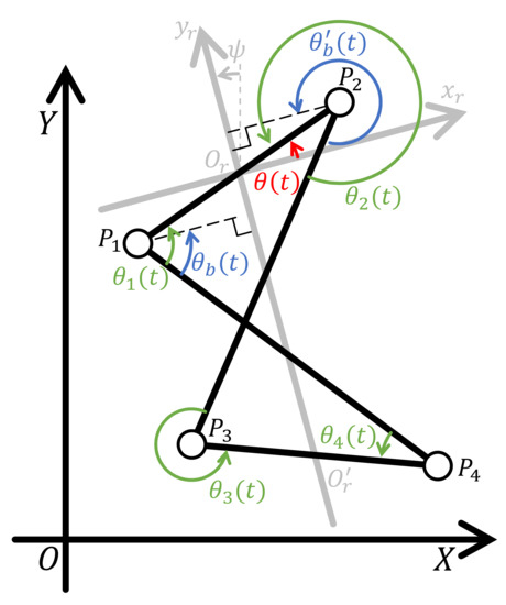
Figure 3.
A schematic figure of the proposed lizard-inspired robot.

Table 1.
Physical parameters.
In Figure 3, the robot switches the support legs appropriately while walking. The support legs are link- and link-. In this paper, the model with link- as the support legs was called “Model-1,” and “Model-2” is that with link-. For each model, the coordinates of each pin joint were formulated as the kinematics of the robot.
The kinematics of Model-1 were derived. In this model, the coordinates of both the pin joint and are known because both joints are fixed on the ground as the support legs. Hence, is also known. Thus, the coordinates of both and were formulated here. From Figure 3:
By the cosine theorem:
where is defined as a square of the distance between the pin joints; that is, . By the bilateration problem:
where is the bilateration matrix, and:
is defined as positive if is to the left of vector , and negative otherwise. Additionally:
Hence, the coordinates of the pin joint and were obtained as follows:
The kinematics of Model-2 were also derived. In this model, the coordinates of both the pin joint and are known because both joints are fixed on the ground as the support legs. Hence, is also known. Thus, the coordinates of both and were formulated here. By the bilateration matrix:
Additionally:
Hence, the coordinates of the pin joint and were obtained as follows:
The kinematics of the robot were formulated. Note that both (1) and (4) are functions of . In addition, Model-1 and Model-2 are switched with one another once .
We then formulated as follows:
Equation (5) is a cosine wave with bias, where is an amplitude, is an angular frequency, and is the bias. These are tuning parameters. In other words, the locomotion control of the lizard robot solves the inverse problems of the parameters that are used to realize the desired locomotion. Our next analyses were based on these parameters, and they were used to solve forward problems. In addition, these parameters are necessary for a mechanical design that satisfies the required specifications.
It is noted that (5) is a periodic function. Therefore, Model-1 and Model-2 also switch periodically. In addition, because the robot has the four-bar linkage mechanism morphology, the robot continues to retain the same kinetic characteristics as long as it is driven by the same model. This suggests that proper analyses during the use of the same models are of little consequence. Hence, for the kinematic characteristics, the differences in the robot’s coordinates in the half period of (5) were compared and formulated.
2.2. Turning-Angle Analysis
The first analysis was with respect to the turning angle. Turning locomotion is generated as long as the that is added is a non-zero value due to the inequality of because the turning angle equals the difference in , as shown in Figure 4. In Figure 4, the black line with a gray axis shows both the initial posture and the posture after one period of the robot, and the purple line with a pale purple axis shows the posture after half of a period of the robot. Meanwhile, the green arrows define the angles of each state, and the red lines show the stride length of the robot and an angle for realizing the stride. Next, we proved that the robot turns with a constant turning angle by adding with a constant value. First, the inequality of per half period by adding with a non-zero value was proven. After that, it was proven that the inequality possesses equality in the first and second half periods. Note that arguments represent the initial time (), the half-period time (), and the one-period time (), respectively.
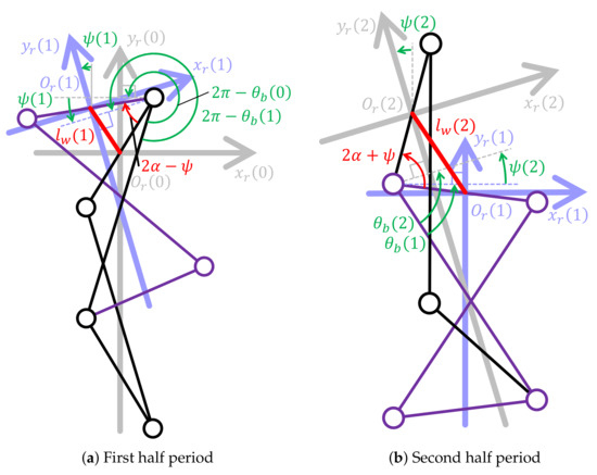
Figure 4.
Variations of the robot’s posture. (a) First half period. (b) Second half period. The black line with a gray axis shows both the initial posture and the posture after one period of the robot, and the purple line with a pale purple shows the posture after half of a period of the robot. Meanwhile, the green arrows define the angles of each state, and the red lines show the stride length of the robot and an angle for realizing the stride. It is shown that equals the difference between and . In addition, it is shown that the relationships between , and and and configure isosceles triangles.
From Figure 4, the difference of in the first half period can be determined as:
Additionally, from Figure 4, the difference in in the second half period can be determined as:
2.3. Stride-Length Analysis
The second analysis was with respect to the stride length. The stride length in this paper was defined as the traveling distance of the robot coordinates with respect to each half period. The robot walks with different stride lengths between the first and second half periods as long as (see Figure 4). Hence, the stride lengths with respect to each half period were formulated.
First, the stride length in the first half period was formulated. From Figure 4, when the robot walks, the relation of and the robot coordinates configure an isosceles triangle because lengths from or to equal . By utilizing the relationship of the isosceles triangle, the stride length in the first half period, say , can be formulated as follows:
Next, the stride length in the second half period was formulated. From Figure 4, the stride length in the second half period, say , can be formulated as follows:
From (8) and (9), the stride length depends on the parameters of the input angle function, as well as the link length, which is a physical parameter of the robot. This means that the stride length can be tuned by the input angle function’s parameters so that the actuator’s specification satisfies a required specification. This also means that the robot’s design influences the maximum limit of the feasible stride length; that is, (8) and (9) become an important index for locomotion control, as well as for the mechanical design.
2.4. Numerical Simulations
The results of the analyses were verified via three numerical simulations. In the numerical simulations, three motions were performed: forward locomotion, clockwise turning locomotion, and counter-clockwise turning locomotion. The numerical simulations were performed using MATLAB 2018b (Update 2 9.5.0.1033004). In the numerical simulations, the positions of each pin joint corresponding to (5) were calculated by (1) and (4). Then, from each calculated coordinate, the turning angle and the stride length were calculated. The physical parameters of the robot are shown in Table 1. The simulation time was set to 4 s for all, and the sampling interval was set to s for all.
The first simulation was for forward locomotion. In this simulation, the parameters of (5) were set as follows:
From (6)–(9), the robot’s turning angle and stride length corresponding to the parameters were 0 rad and 25 mm, respectively. Our simulation results are shown in Figure 5, Figure 6 and Figure 7. The results show that our analyses satisfy the simulation results of forward locomotion.
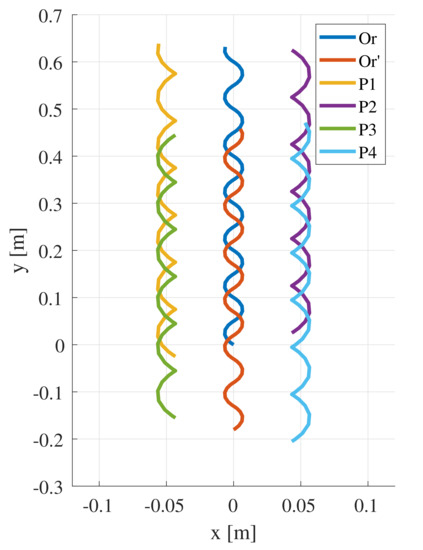
Figure 5.
The trajectories of each joint in the simulation for forward locomotion. The simulation results show that the robot moves forward by setting .
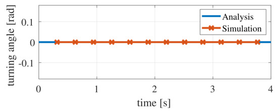
Figure 6.
The time variation of the turning angle in the simulation for forward locomotion. Since the turning angle indicates 0 rad, the simulation results show that the robot moves forward by setting .
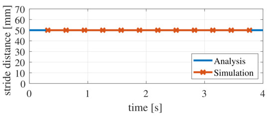
Figure 7.
The time variation of the stride length in the simulation for forward locomotion. The simulation results show that the robot walks with a constant stride length.
The second simulation was for clockwise turning locomotion. In this simulation, the parameters of (5) were set as follows:
From (6)–(9), corresponding to the parameters, the robot’s turning angle was rad, and the stride lengths in the first and second half periods were 61.2 and 37.8 mm, respectively. The simulation results are shown in Figure 8, Figure 9 and Figure 10. The results show that the our analyses satisfy the simulation results of clockwise turning locomotion.
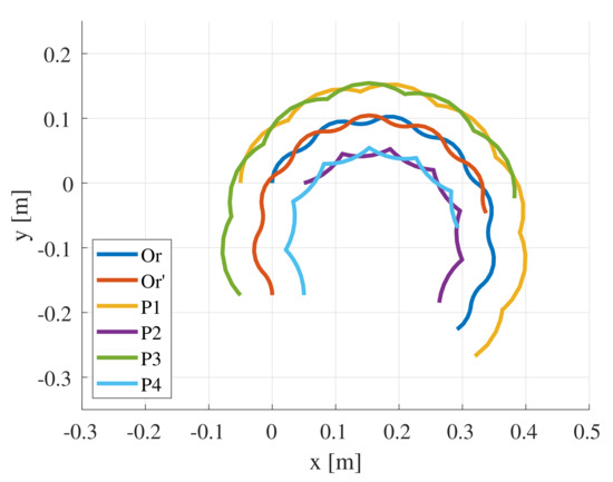
Figure 8.
The trajectories of each joint in the simulation for clockwise turning locomotion. The simulation results show that the robot turns to the right by setting .
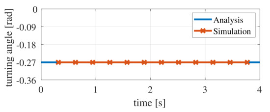
Figure 9.
The time variation of the turning angle in the simulation for clockwise turning locomotion. Since the turning angle indicates rad, the simulation results show that the robot turns to the right by setting .
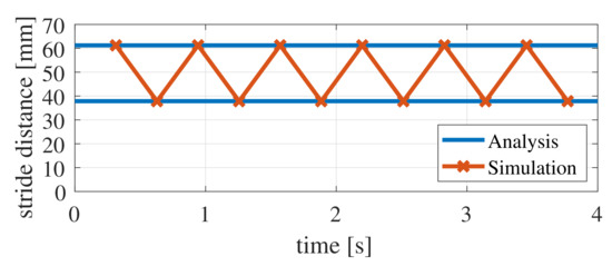
Figure 10.
The time variation of the stride length in the simulation for the clockwise turning locomotion. The simulation results show that the robot walks with different stride lengths in each half period.
The third simulation was for counter-clockwise turning locomotion. In this simulation, the parameters of (5) were set as follows:
From (6)–(9), corresponding to the parameters, the robot’s turning angle was 0.27 rad, and the stride lengths in the first and second half periods were 37.8 and 61.2 mm, respectively. The simulation results are shown in Figure 11, Figure 12 and Figure 13. The results show that our analyses satisfy the simulation results of counter-clockwise turning locomotion.
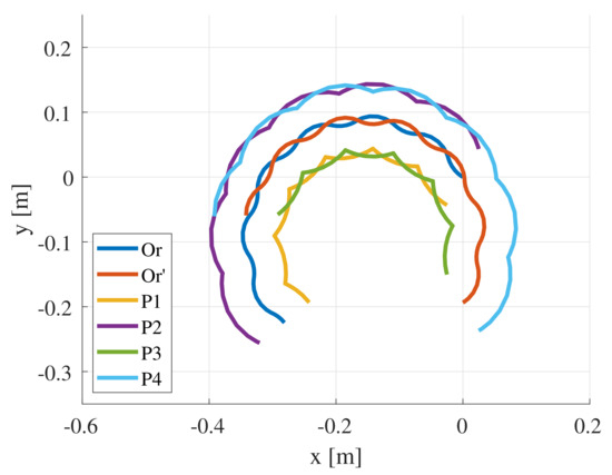
Figure 11.
The trajectories of each joint in the simulation for counter-clockwise turning locomotion. The simulation results show that the robot turns to the left by setting .
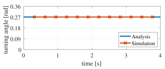
Figure 12.
The time variation of the turning angle in the simulation for the counter-clockwise turning locomotion. Since the turning angle indicates 0.27 rad, the simulation results show that the robot turns to the left by setting .
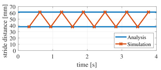
Figure 13.
The time variation of the stride length in the simulation for counter-clockwise turning locomotion. The simulation results show that the robot walks with different stride lengths in each half period.
3. Design and Fabrication of the Lizard-Type Robot
In this section, the lizard-inspired robot with a new morphology consisting of a four-bar linkage mechanism was designed and fabricated. When designing the robot, two main issues were addressed. Solutions to the issues are shown herein, and the robot was then designed and fabricated.
The first main issue was the switching method between the supporting and idling legs. A general multi-legged robot walks by switching the roles of each leg into those of the supporting leg and the idling leg, synchronizing them appropriately. In addition, proper gripping is preferred for the supporting leg, while full slipping with lower load forces (e.g., friction forces) is preferred for the idling leg. A general multi-legged robot switches the supporting and idling legs when the leg contacts the ground. However, the robot proposed in this paper consists of a planar closed-linkage mechanism, and each pin joint works as a leg. Thus, to realize the switching of the supporting and idling legs through the up–down movement of the legs (similarly to a general multi-legged robot), pin joints are required in order to drive them in the axial direction. A mechanism for satisfying this requirement could be designed. However, such a mechanism would easily generate collisions between linkages. Driving the pin joints in the axial direction represents driving the connected links of the joints. Thus, two links in the front and back, as well as another two links crossing one another, move perpendicularly to the plane. Moreover, it is easy to imagine that the movements result in collisions between the links. In order to avoid collisions, it is necessary to design a complex shape for the linkage and pin joints, and such a mechanism design is too difficult to prototype.
As a solution for the first main issue, we propose a shuffle-walking method. The shuffle-walking method allowed us to design a robot consisting of a simple planar linkage mechanism using a claw-shaped leg mechanism. Generally, a claw is grippy in the claw direction, but is otherwise slippery. A textured plane, such as a carpet, was supposed, and the claw was designed so that its tip was pointed in the diagonal direction of the carpet surface; additionally, it was equipped so that the tip was pointed in the backward direction with respect to the robot. The design used a leg mechanism that is grippy in the backward direction and slippery in the forward direction. Each pin joint possesses a claw-shaped leg mechanism. When rotating the driving link on the carpet surface, one pin joint generates a translational force in the backward direction, and the opposite joint generates force in the forward direction. The pin joint generating the force in the backward direction stays on-site because the claw is hooked onto the carpet surface. However, the opposite joint slips on the carpet surface and moves forward, since the force works in the slippery direction for the claw. Thus, shuffle-walking is realized.
The second main issue was the location for the installment of an actuator. In the proposed robot model, the input angle function was set on the robot coordinates for the robot’s locomotion. Hence, the robot’s actuator in the design also had to be installed on the robot’s coordinate (i.e., on ). To install the actuator on the robot’s coordinate, and have to be physically connected by a link. However, the distance between and varies, corresponding to the angle of the input angle function .
As a solution for the second main issue, a linear sliding rod was adopted to connect the pin joints at and . In particular, was designed as a pin joint to install the actuator, and was designed as a sliding joint. Meanwhile, and were connected by a sliding rod.
Figure 14 shows the CAD designs of the robot. Figure 15 shows photographs of the developed robot. As shown in Figure 14 and Figure 15, the robot possessed the morphology of the four-bar linkage mechanism consisting of one sliding rod, two “S”-shaped links, and two “I”-shaped links, and each link was connected by a linear bush and bearings. The links were fabricated with a 3D printer, and the claw-shaped legs with aluminum were fabricated with a laser cutter. Dynamixel XM430-W350-T, which was developed by ROBOTIS, was installed as the actuator. Table 2 shows the specifications of Dynamixel XM430-W350-T. OpenCM 9.04-C with an Expansion Board, also developed by ROBOTIS, was adopted as a control board. Table 3 shows the specifications of OpenCM 9.04-C. An external power supply provided DC12 V for the power source of both the actuator and the control board. Figure 15c and Figure 16 are photographs of the claw-shaped leg mechanism, with the right-hand direction in the picture being the direction of travel of the robot. When the leg moves in the direction of motion, it slides easily on the ground because the claw does not grip. In other words, the legs move forward. On the other hand, when the leg moves backward, it does not slide because the claw gets caught on the ground. In other words, the legs do not move backward. The roles of these legs are switched according to the direction of rotation of the actuator.
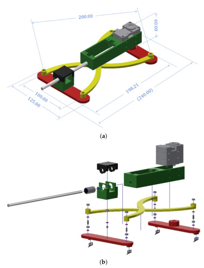
Figure 14.
The CAD design of the robot: (a) the CAD design and dimensions; (b) the developmental diagram.
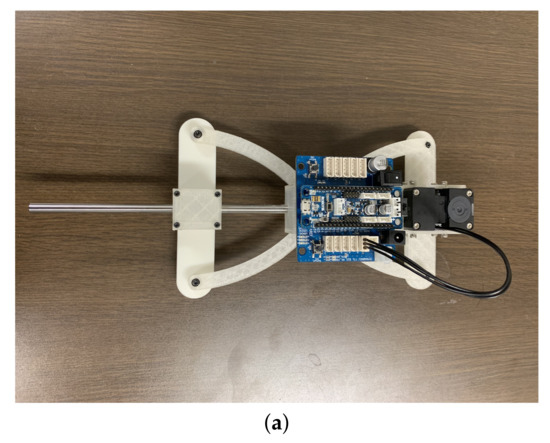

Figure 15.
Photographs of the fabricated robot: (a) top view; (b) side view; (c) the claw-shaped leg mechanism.
Table 2.
Specifications of XM430-W350-T.
Table 3.
Specifications of OpenCM 9.04-C.
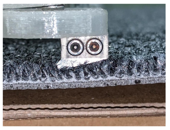
Figure 16.
Photograph of the ground contact between the leg mechanism and the carpet surface. The right-hand direction is the direction of travel. The claw does not get caught in the direction of travel, so the leg can slide. In other words, the robot moves forward. In the opposite direction, the legs cannot slide because the claws get caught. In other words, it does not move backward.
4. Results of the Experiments and Discussion
In this section, the effectiveness of the developed robot was verified through four experiments. The experiments verified both the effectiveness of the claw-shaped leg mechanism and the locomotion performance of the robot. One of the experiments was conducted to verify the effectiveness of the claw-shaped leg mechanism. Another three experiments were conducted to verify the locomotion performance of the developed robot. To verify the locomotion performance, a motion-capture camera system (V120 Trio developed by OptiTrack, shown in Figure 17) captured the markers equipped on the robot. The markers were installed on , and of the robot, as shown in Figure 18. The frame rate of the motion-capture system was set to 120 fps. MATLAB 2018b Update2 (9.5.1033004) was used to process the captured experimental data. All experiments were performed on a flat carpet surface.
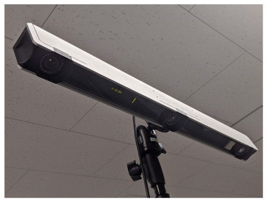
Figure 17.
The motion-capture camera system of V120 Trio, developed by OptiTrack.
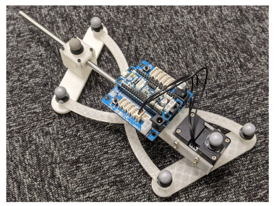
Figure 18.
The installation locations of the markers. The six markers were installed on , , , and of the robot.
4.1. Effectiveness of the Claw-Shaped Leg
The first experiment verified the effectiveness of the claw-shaped leg mechanism. The purpose of this experiment was to prove that the claw-shaped leg mechanism realized the difference in slipperiness between the forward and backward directions. Walking with a shuffle requires two states of grip in the supporting leg side and the slippery idling leg side of the robot. To prove that the developed robot satisfies this requirement, the maximum static frictional forces in both the forward and the backward direction were measured and compared. Figure 19 shows the environment of the experiment. The static frictional forces were measured by pulling the robot with weights, as shown in Figure 19. The static frictional forces were identified as forces at the beginning of the slip. Table 4 shows the results of the experiment.
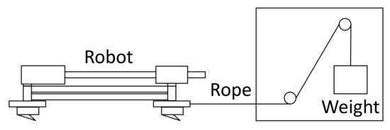
Figure 19.
A schematic figure of the static frictional force measurement experiment.
Table 4.
The static frictional forces measured in both the forward and backward directions.
Table 4 shows that the proposed claw-shaped leg mechanism provided an 85.26 N difference for the maximum static frictional forces between the forward and backward directions on the carpet surface. Hence, the proposed claw-shaped leg mechanism was able to generate enough slipperiness for shuffle-walking.
4.2. Forward Locomotion
The second experiment verified the forward locomotion of the robot. The purpose of this experiment was to prove that the robot was capable of repeating the supposed forward locomotion. The parameters of the input angle function for the experiment were set as follows:
The parameters represent the robot moving forward in a straight line. The locomotion time of the robot was set to 4 s. Forward locomotion was repeated 10 times. Table 5 shows the results of the experiments. In Table 5, “traveling distance” is defined as the distance from the starting point to the terminal point of . Additionally, Figure 20 shows the trajectories of each marker in the eighth experiment. Figure 21 shows a snapshot of the forward locomotion experiments.
Table 5.
The results of the forward locomotion experiments.
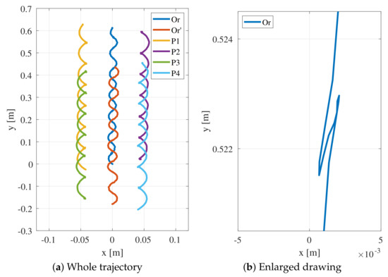
Figure 20.
The trajectory of each marker in the eighth experiment of the forward locomotion experiment. (a) The overall view of the trajectories. (b) An enlarged view of the trajectory of . The robot coordinate moved backward marginally because of the flexure of the carpet.
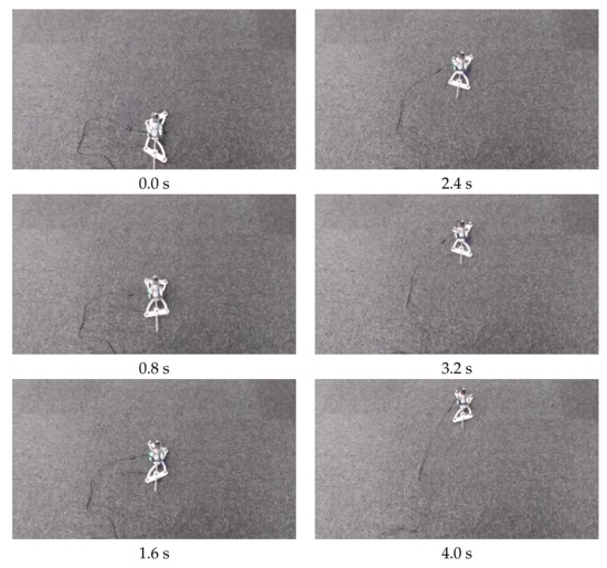
Figure 21.
Snapshots of the forward locomotion experiment.
From Table 5, the average of the 10 forward locomotion experiments was 610.67 mm, and the standard deviation was 2.44 mm. Hence, the fabricated robot possessed high repeatability for forward locomotion with respect to the parameters of the input angle function. In addition, the ideal distance of the forward locomotion obtained with the numerical simulation was 632.90 mm, and the error ratio between the average of the experiments and the ideal distance was 3.51%. Therefore, the proposed claw-shaped leg mechanism is effective for the developed robot, and the developed robot is capable of walking without the supporting legs slipping.
The cause of the 3.51% error ratio was the backward movement of the robot due to the deflection of the carpet. As shown in Figure 22, the carpet consisted of cushioned fibers. The supporting legs kicked the ground to walk, and the fibers were deflected. Due to this deflection, the robot moved backward marginally. This backward motion was the cause of the error. In fact, Figure 20b shows that the robot moved backward marginally. Adding this backward distance to the traveling distance, the total distance became 636.83 mm, and the error ratio between the ideal distance and the total distance was 0.62%. This is a vast improvement in the accuracy. Hence, the error of the traveling distance caused the backward motion of the robot due to the flexure of the carpet.
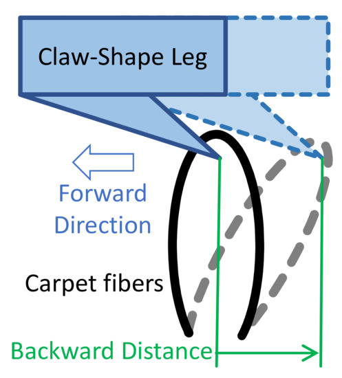
Figure 22.
A schematic figure of the deflection generated by both walking and the fiber construction of the carpet. The supporting legs kicked the ground to walk, and the fibers were deflected. Due to this deflection, the robot moved backward marginally.
4.3. Clockwise Turning Locomotion
The third experiment verified the clockwise turning locomotion of the robot. The purpose of this experiment was to prove that the robot was capable of repeating clockwise turning locomotion. The parameters of the input angle function for the experiment were set as follows:
The parameters show that the robot turned in the clockwise direction. The locomotion time of the robot was set to 4 s. Clockwise turning locomotion was repeated 10 times. Table 6 shows the results of the experiments. Figure 23 shows the trajectories of each marker in the ninth experiment, where the “✕” marks represent the locations of the robot coordinate with respect to each half period of the input angle function. Figure 24 shows the time variation of the relative angle of the “✕” marks in Figure 23, that is, the time variation of the turning angle in the ninth clockwise turning locomotion. Figure 25 shows a snapshot of the clockwise turning locomotion experiments.
Table 6.
The results of the clockwise turning locomotion experiments.
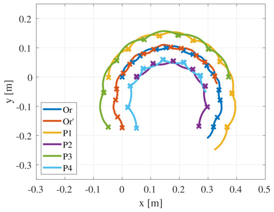
Figure 23.
The trajectories of each marker in the ninth experiment of the clockwise turning locomotion experiment. The “✕” marks represent the locations of the robot coordinate with respect to each half period of the input angle function. The relative angles of the “✕” marks (colored in blue) are the turning angles of the robot.
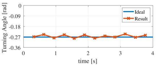
Figure 24.
The time variation of the turning angle in the ninth clockwise turning locomotion experiment.
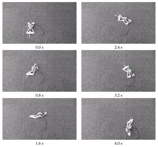
Figure 25.
Snapshots of the clockwise turning locomotion experiment.
From Table 6, it can be seen that the average of the 10 clockwise turning locomotion experiments was rad, with a standard deviation of 0.001 rad. Hence, the fabricated robot possesses high repeatability regarding clockwise turning locomotion with respect to the parameters of the input angle function. In addition, the ideal turning angle of the clockwise turning locomotion obtained by the kinematics analysis was rad, and the error ratio between the average of the experiments and the ideal turning angle was 3.16%. Since the error ratio was almost equal to the value in the forward locomotion experiment, the error in this experiment was also caused by the deflection of the carpet. Figure 23 shows that the robot turned in a clockwise direction. Figure 24 shows that the turning angle during the clockwise turning locomotion largely remained at the ideal angle. Hence, this experiment’s results guarantee that the fabricated robot is capable of turning in a clockwise direction with high accuracy.
4.4. Counter-Clockwise Turning Locomotion
The fourth experiment verified the counter-clockwise turning locomotion of the robot. The purpose of this experiment was to prove that the robot was capable of repeating the counter-clockwise turning locomotion. The parameters of the input angle function for the experiment were set as follows:
The parameters show that the robot turned in a counter-clockwise direction. The locomotion time of the robot was set to 4 s. The counter-clockwise turning locomotion was repeated 10 times. Table 7 shows the results of the experiments. Figure 26 shows the trajectories of each marker in the 10th experiment, where the “✕” marks represent the locations of the robot coordinate with respect to each half period of the input angle function. Figure 27 shows the time variation of the relative angle of the “✕” marks in Figure 26, that is, the time variation of the turning angle in the 10th counter-clockwise turning locomotion. Figure 28 shows a snapshot of the counter-clockwise turning locomotion experiments.
Table 7.
The results of the counter-clockwise turning locomotion experiments.
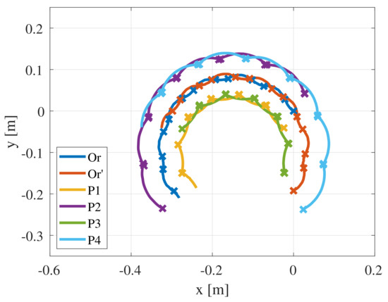
Figure 26.
The trajectories of each marker in the 10th experiment of the counter-clockwise turning locomotion experiment. The “✕” marks represent the locations of the robot coordinate with respect to each half period of the input angle function. The relative angles of the “✕” marks (colored in blue) are the turning angles of the robot.
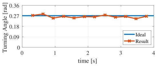
Figure 27.
The time variation of the turning angle in the 10th counter-clockwise turning locomotion experiment.
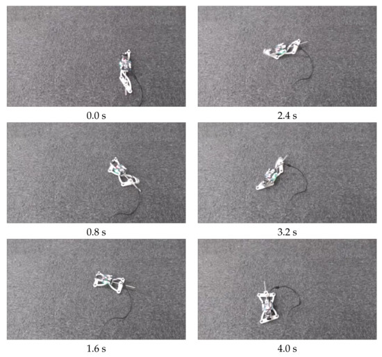
Figure 28.
Snapshots of the counter-clockwise turning locomotion experiment.
From Table 7, it can be seen that the average of the 10 counter-clockwise turning locomotion experiments was 0.261 rad, with a standard deviation of 0.001 rad. Hence, the fabricated robot possesses high repeatability regarding the counter-clockwise turning locomotion with respect to the parameters of the input angle function. In addition, the ideal turning angle of the counter-clockwise turning locomotion obtained by the kinematic analysis was 0.271 rad, and the error ratio between the average of the experiments and the ideal turning angle was 3.53%. Since the error ratio was almost equal to the value in the forward locomotion experiment, the error in this experiment was also caused by the deflection of the carpet. Figure 26 shows that the robot turned in the counter-clockwise direction. Figure 27 shows that the turning angle during the counter-clockwise turning locomotion largely remained at the ideal angle. Hence, the experimental results guarantee that the fabricated robot is capable of turning in a counter-clockwise direction with high accuracy.
4.5. Discussion
We will discuss how this error can be improved. For this situation, we consider that the method of adding the amount of carpet warping to the motor drive amount is effective. In this experiment, the same error rate was observed in all walking patterns. Therefore, it is assumed that the cause of the error in each walking pattern is the deflection of the carpet, and the amount of the distortion is approximately the same. Therefore, it is possible to improve the error by adding the amount of warping to the motor drive amount.
When the ground conditions are different, the leg mechanism must be improved. The leg mechanism developed in this paper cannot be used to walk correctly on a slippery surface, such as a wooden floor. Therefore, it is desirable to develop a more advanced leg mechanism, such as a leg mechanism that can use suction.
5. Conclusions
A new type of lizard-inspired robot that is capable of walking with only a single actuator was developed and verified via four experiments. A lizard possesses an I-type morphology. It improves its walking efficiency through the flexion movement of the trunk instead of through leg locomotion, especially when running quickly. This characteristic enabled us to decrease the number of actuators, that is, to allude to the feasibility of a multi-legged robot that is driven by only a single actuator. Realizing this robot can help in resolving the issue of the energy efficiency of multi-legged robots. The novelty of our robot lies in its ability to mimic the morphology of a lizard with a four-bar linkage mechanism. This novelty provides the robot with an appropriate means of walking in which its support legs do not slip. This also allowed us to formulate proper kinematic characteristics via kinematic analyses, which are much simpler than dynamic analyses. The conclusions of this paper were supported by three processes.
The first process was kinematic analysis, where we defined our own robot model and formulated the kinematic characteristics based on the period of the input angle function. Based on these ideas, the turning angle and the stride length of the robot were formulated. In addition, the results of the kinematic analysis were guaranteed through three numerical simulations.
The second process was the design and the fabrication of the robot. For the robot’s design, two main issues were addressed. The first issue was the switching method between the support and swing legs. To solve this issue, we proposed a shuffle-walking method using a claw-shaped leg mechanism. The second issue was the location of the actuator. As a solution to the second main issue, a linear sliding rod was adopted to connect the two points with varying distances. One side was designed as a pin joint for the actuator, and the other side was a sliding joint. The robot was then fabricated according to these solutions.
The third process was experimental verification. The effectiveness of the fabricated robot was verified through four experiments. The first experiment verified the effectiveness of the claw-shaped leg mechanism. The maximum static frictional force in the longitudinal direction was measured, and the experimental results showed that the proposed leg mechanism generated an 85.26 N difference in the static frictional force. The second experiment verified the forward locomotion performance. The trajectories of the markers attached to the robot were measured with a motion-capture system. The experimental results showed that the robot was able to move forward with a 3.51% error compared to the kinematic analysis. The third and fourth experiments verified the clockwise and counter-clockwise turning locomotions, respectively. In the same way as in the second experiment, the trajectories of the markers were measured, and the turning angles of the robot were calculated. The error ratios were 3.16% in clockwise locomotion and 3.53% in counter-clockwise turning locomotion. The results of these experiments proved that the fabricated lizard-inspired robot is capable of achieving its expected performance.
In future work, our next goal is to design a motion control system, such as trajectory tracking control, based on the kinematic analyses formulated in this paper. The bias of the input function can be controlled so that it follows a reference trajectory, such as a straight line or a circle. In addition, we are also working on developing more advanced leg mechanisms. The prototype developed in this paper can walk only on a flat surface. However, since a real environment is uneven, we will develop a new leg mechanism that can cope with the unevenness.
Author Contributions
S.N. and Y.A.: analysis, simulation, design, and implementation of the robot. H.I. and N.K.: project administration. All authors have read and agreed to the published version of the manuscript.
Funding
This research was funded by the NSK Foundation for the Advancement of Mechatronics, JSPS KAKENHI, grant number 21K14107, and the Research Institute for Science and Technology of Tokyo Denki University, grant number Q21T-05.
Institutional Review Board Statement
Not applicable.
Informed Consent Statement
Not applicable.
Conflicts of Interest
The authors declare no conflict of interest.
References
- Kazemi, H.; Majd, V.J.; Moghaddam, M.M. Modeling and robust backstepping control of an underactuated quadruped robot in bounding motion. Robotica 2013, 31, 423. [Google Scholar] [CrossRef]
- Silva, M.F.; Machado, J.T. Kinematic and dynamic performance analysis of artificial legged systems. Robotica 2008, 26, 19. [Google Scholar] [CrossRef]
- Acosta-Calderon, C.A.; Mohan, R.E.; Zhou, C.; Hu, L.; Yue, P.K.; Hu, H. A modular architecture for humanoid soccer robots with distributed behavior control. Int. J. Humanoid Robot. 2008, 5, 397–416. [Google Scholar] [CrossRef]
- Bartsch, S.; Birnschein, T.; Römmermann, M.; Hilljegerdes, J.; Kühn, D.; Kirchner, F. Development of the six-legged walking and climbing robot SpaceClimber. J. Field Robot. 2012, 29, 506–532. [Google Scholar] [CrossRef]
- Estremera, J.; Cobano, J.A.; De Santos, P.G. Continuous free-crab gaits for hexapod robots on a natural terrain with forbidden zones: An application to humanitarian demining. Robot. Auton. Syst. 2010, 58, 700–711. [Google Scholar] [CrossRef]
- Moro, F.L.; Spröwitz, A.; Tuleu, A.; Vespignani, M.; Tsagarakis, N.G.; Ijspeert, A.J.; Caldwell, D.G. Horse-like walking, trotting, and galloping derived from kinematic Motion Primitives (kMPs) and their application to walk/trot transitions in a compliant quadruped robot. Biol. Cybern. 2013, 107, 309–320. [Google Scholar] [CrossRef]
- Sanz-Merodio, D.; Garcia, E.; Gonzalez-de Santos, P. Analyzing energy-efficient configurations in hexapod robots for demining applications. Ind. Robot Int. J. 2012, 39, 357–364. [Google Scholar] [CrossRef]
- De Santos, P.G.; Garcia, E.; Ponticelli, R.; Armada, M. Minimizing energy consumption in hexapod robots. Adv. Robot. 2009, 23, 681–704. [Google Scholar] [CrossRef]
- Roy, S.S.; Pratihar, D.K. Dynamic modeling, stability and energy consumption analysis of a realistic six-legged walking robot. Robot. Comput. Integr. Manuf. 2013, 29, 400–416. [Google Scholar] [CrossRef]
- Jansen, T. The Great Pretender; 010 Publishers: Rotterdam, The Netherlands, 2007. [Google Scholar]
- Komoda, K. A study of availability and extensibility of Theo Jansen mechanism toward climbing over bumps. In Proceedings of the 21st Annual Conference of the Japanese Neural Networks Society, Okinawa, Japan, 15–17 December 2011; pp. 192–193. [Google Scholar]
- Komoda, K.; Wagatsuma, H. A proposal of the extended mechanism for theo jansen linkage to modify the walking elliptic orbit and a study of cyclic base function. In Proceedings of the 7th Annual Dynamic Walking Conference (DWC’12), Pittsburgh, PA, USA, 21–24 May 2012. [Google Scholar]
- Moldovan, F.; Dolga, V. Analysis of Jansen walking mechanism using CAD. In Solid State Phenomena; Trans Tech Publications: Stafa-Zurich, Switzerland, 2010; Volume 166, pp. 297–302. [Google Scholar]
- Ingram, A.J. A New Type of Mechanical Walking Machine; Rand Afrikaans University: Johannesburg, South Africa, 2006. [Google Scholar]
- Giesbrecht, D.; Wu, C.Q. Dynamics of Legged Walking Mechanism “Wind Beast”. In Proceedings of the Dynamic Walking Conference, Burnaby, BC, Canada, 8–11 June 2009. [Google Scholar]
- Liu, C.H.; Lin, M.H.; Huang, Y.C.; Pai, T.Y.; Wang, C.M. The development of a multi-legged robot using eight-bar linkages as leg mechanisms with switchable modes for walking and stair climbing. In Proceedings of the 2017 3rd International Conference on Control, Automation and Robotics (ICCAR), Nagoya, Japan, 24–26 April 2017; pp. 103–108. [Google Scholar]
- Nansai, S.; Elara, M.R.; Iwase, M. Dynamic analysis and modeling of Jansen mechanism. Procedia Eng. 2013, 64, 1562–1571. [Google Scholar] [CrossRef]
- Nansai, S.; Rojas, N.; Elara, M.R.; Sosa, R. Exploration of adaptive gait patterns with a reconfigurable linkage mechanism. In Proceedings of the 2013 IEEE/RSJ International Conference on Intelligent Robots and Systems, Tokyo, Japan, 3–7 November 2013; pp. 4661–4668. [Google Scholar]
- Nansai, S.; Rojas, N.; Elara, M.R.; Sosa, R.; Iwase, M. On a Jansen leg with multiple gait patterns for reconfigurable walking platforms. Adv. Mech. Eng. 2015, 7, 1687814015573824. [Google Scholar] [CrossRef]
- Nansai, S.; Rojas, N.; Elara, M.R.; Sosa, R.; Iwase, M. A novel approach to gait synchronization and transition for reconfigurable walking platforms. Digit. Commun. Netw. 2015, 1, 141–151. [Google Scholar] [CrossRef]
- Zarrouk, D.; Fearing, R.S. Compliance-based dynamic steering for hexapods. In Proceedings of the 2012 IEEE/RSJ International Conference on Intelligent Robots and Systems, Vilamoura-Algarve, Portugal, 7–12 October 2012; pp. 3093–3098. [Google Scholar]
- Zarrouk, D.; Fearing, R.S. Cost of locomotion of a dynamic hexapedal robot. In Proceedings of the 2013 IEEE International Conference on Robotics and Automation, Karlsruhe, Germany, 6–10 May 2013; pp. 2548–2553. [Google Scholar]
- Zarrouk, D.; Fearing, R.S. 1star, a one-actuator steerable robot. In Proceedings of the 2014 IEEE International Conference on Robotics and Automation (ICRA), Hong Kong, China, 31 May–7 June 2014; p. 2569. [Google Scholar]
- Zarrouk, D.; Pullin, A.; Kohut, N.; Fearing, R.S. STAR, a sprawl tuned autonomous robot. In Proceedings of the 2013 IEEE International Conference on Robotics and Automation, Karlsruhe, Germany, 6–10 May 2013; pp. 20–25. [Google Scholar]
- Karydis, K.; Zarrouk, D.; Poulakakis, I.; Fearing, R.S.; Tanner, H.G. Planning with the STAR (s). In Proceedings of the 2014 IEEE/RSJ International Conference on Intelligent Robots and Systems, Chicago, IL, USA, 14–18 September 2014; pp. 3033–3038. [Google Scholar]
- Zarrouk, D.; Yehezkel, L. Rising STAR: A highly reconfigurable sprawl tuned robot. IEEE Robot. Autom. Lett. 2018, 3, 1888–1895. [Google Scholar] [CrossRef]
- Zarrouk, D.; Mann, M.; Degani, N.; Yehuda, T.; Jarbi, N.; Hess, A. Single actuator wave-like robot (SAW): Design, modeling, and experiments. Bioinspiration Biomim. 2016, 11, 046004. [Google Scholar] [CrossRef] [PubMed]
- Drory, L.H.; Zarrouk, D. Locomotion dynamics of a miniature wave-like robot, modeling and experiments. In Proceedings of the 2019 International Conference on Robotics and Automation (ICRA), Montreal, QC, Canada, 20–24 May 2019; pp. 8422–8428. [Google Scholar]
- Yang, M.; Kang, R.; Chen, Y. A Highly Mobile Crawling Robot Inspired by Hexapod Insects. In Proceedings of the 2019 IEEE International Conference on Robotics and Biomimetics (ROBIO), Dali, China, 6–8 December 2019; pp. 1797–1802. [Google Scholar]
- Hirose, S.; Umetani, Y. The basic considerations on energetic efficiencies of walking vehicle. Trans. Soc. Instrum. Control. Eng. 1979, 15, 928–933. [Google Scholar] [CrossRef][Green Version]
- Niimi, H.; Koike, M.; Takeuchi, S.; Douhara, N. Study of biomimetic walking robots using the trunk of the body. In Proceedings of the Annual Conference of the Institute of Systems, Control and Information Engineers, Kyoto, Japan, 19–21 May 2010; Volume SCI10, p. 182. [Google Scholar] [CrossRef]
- Hirofumi, N.; Kensuke, M. 2P1-M08 Biomimetics Mobile Robot using the Trunk of the Body: Ahead, Astern and Turning of Lizard Type Robot(Bio-Mimetics and Bio-Mechatronics). In Proceedings of the JSME Annual Conference on Robotics and Mechatronics (Robomec), Okayama, Japan, 26–28 May 2011; Volume 2011. [Google Scholar] [CrossRef]
- Niimi, H.; Suzaki, F.; Murai, K. 2A2-T04 Performance Test of Lizard Robot in the Field(Walking Robot (2)). In Proceedings of the JSME Annual Conference on Robotics and Mechatronics (Robomec), Hamamatsu, Japan, 27–29 May 2012; Volume 2012. [Google Scholar] [CrossRef]
- Kawakami, Y.; Kamamichi, N. 2P1-F04 Motion Analysis of Lizard Type Quadruped Robots(Biorobotics (2)). In Proceedings of the JSME Annual Conference on Robotics and Mechatronics (Robomec), Tsukuba, Japan, 22–25 May 2013; Volume 2013. [Google Scholar] [CrossRef]
- Suzuki, H.; Wakikawa, K.; Kamamichi, N. Motion control of lizard-type quadruped. In Proceedings of the JSME Annual Conference on Robotics and Mechatronics (Robomec), Yokohama, Japan, 8–11 June 2016; Volume 2016, p. 1A2-07b6. [Google Scholar] [CrossRef]
- Nansai, S.; Elara, M.R.; Iwase, M. Speed Control of Jansen Linkage Mechanism for Exquisite Tasks. J. Adv. Simul. Sci. Eng. 2016, 3, 47–57. [Google Scholar] [CrossRef]
- Rojas, N.; Thomas, F. Application of distance geometry to tracing coupler curves of pin-jointed linkages. J. Mech. Robot. 2013, 5, 021001. [Google Scholar] [CrossRef]
- Rojas, N.S.; Thomas, F. A coordinate-free approach to tracing the coupler curves of pin-jointed linkages. In Proceedings of the International Design Engineering Technical Conferences and Computers and Information in Engineering Conference, Washington, DC, USA, 28–31 August 2011; Volume 54839, pp. 417–426. [Google Scholar]
- Rojas, N.; Thomas, F. On closed-form solutions to the position analysis of Baranov trusses. Mech. Mach. Theory 2012, 50, 179–196. [Google Scholar] [CrossRef]


Publisher’s Note: MDPI stays neutral with regard to jurisdictional claims in published maps and institutional affiliations. |
© 2021 by the authors. Licensee MDPI, Basel, Switzerland. This article is an open access article distributed under the terms and conditions of the Creative Commons Attribution (CC BY) license (https://creativecommons.org/licenses/by/4.0/).