A Dynamic Model Updating Method with Thermal Effects Based on Improved Support Vector Regression

Abstract

The dynamic modeling of structures in a thermal environment has become a new research topic in structural dynamics. The amount of calculation caused by the complexity of the structure and the size of the FEM, which increase the difficulty in modeling the structural dynamic thermal effects are considered. In this study, model updating in thermal temperature environment is proposed based on the hierarchical method and improved SVR, and an iterative procedure is presented. First, the dynamic problem of structure under a thermal environment is classified into a thermal model and a structural dynamic model, and they are both constructed with the FE method. As a result, the model updating process is conducted for both the thermal model and structural dynamic model. Different from the variables in other model updating methods, the updating variables, which are composed of the mechanical characteristics and thermal parameters, in the proposed method are dominated by the temperature distribution of the structure. A surrogate model based on improved SVR is adopted in the hierarchical model updating approach to make the updating process more efficient. Finally, the improved SVR method is validated on a typical nonlinear function, and the proposed method is validated by updating the model of an elastic thin plate and a wing structure in a thermal environment.

1. Introduction

The increase in speed of the aircraft often leads to an increase in temperature, which are always subjected to an extremely high surface temperature and large temperature gradients, which can seriously affect the modal characteristics of the structure and can affect the aeroelastic and aeroservoelastic stability of the vehicles. Usually, the FE model analysis methods are to be employed to predict structural dynamic properties. Hence, accurately determining the modal characteristics of these structures at elevated temperatures is vital. However, there is a coupling effect between structural vibration and temperature [1]. On the one hand, the change of structural temperature distribution with time causes structural vibration [2]; on the other hand, the mechanical energy is converted into thermal energy during structural vibration, which changes the state of structural temperature distribution [3]. As this coupling effect is very weak, for large complex mechanical systems, especially in high temperature environments, the temperature change caused by structural vibration is negligible. Therefore, when dealing with structural dynamics in a thermal environment, temperature is generally considered as the equivalent load acting on the vibration equation, ignoring the effect of the thermal-elastic coupling effect.

The identification of thermal parameters is an important element of the inverse heat conduction problem and is necessary to obtain accurate temperature distributions, which are widely used in aerospace, power engineering, nuclear physics and other fields. Sawaf and Özisik used Levenberg-Marquardt method to identify the thermal conductivity of anisotropic materials [4]. A 3–D transient inverse heat conduction problem is solved with the CGM and the general-purpose commercial code CFX4.2-based inverse algorithm to estimate the unknown boundary heat flux in any 3-D irregular domain [5]. Gosselin summarized the application of genetic algorithms to heat transfer problems, mainly for thermal system design, heat transfer inverse problems and heat transfer correlations [6]. Sahoo and his colleagues used segment-by-segment linear fit, polynomial fit and a cubic spline approach to investigate the heat transfer inverse problem for hypervelocity vehicle test data, and the results showed that only the polynomial fit and the cubic spline approach obtained results that were consistent with the test data [7] The joint PPDF of the heat source values at consecutive time points is computed with Bayes’ formula, and the MCMC simulation method is used to compute the MAP and posterior mean estimates of the heat source [8]. Cui [9] proposed a complex variable differentiation method to calculate the sensitivity matrix, the thermophysical properties of the material with temperature are identified by the conjugate gradient method, the functional form of the unknown parameters is not required in the calculation, and the computational efficiency and computational accuracy of the algorithm are verified using numerical calculations. Cappelli and his coworkers proposed a MSIS to identify the parameters involved in the elastic, viscoelastic in presence of uncertainty and by considering more general piezo-electric materials at each pertinent scale of the structure [10,11]. This means that the MSIS is able not only to identify the parameters involved into the material law at the macroscopic scale but also those parameters involved at the microscopic scale of the constitutive phases of the composite [12]. But these works based on Genetic Algorithms which cost a significant computational resources and computational time. This problem is largely overcome by the use of a metamodel as a surrogate for the physical model.

The frequently used approaches for identifying thermophysical parameters currently assume that the thermophysical parameters of the material are a constant or are of a known functional form that changes with temperature [13]. However, in practical engineering, the rules of the thermophysical parameters changing with temperature are usually more complicated. On the basis of the steady-state temperature distribution, this paper proposes an identification approach for thermophysical parameters based on support vector regression. In contrast with the traditional identification approaches, we assume the thermophysical parameters are in a format of the primary function linear combination group, in which the primary function can be expressed through surrogate model. The common construction methods for the surrogate model are [14]: Response Surface Method, Moving Least Square, Artificial Neural Networks, Radial Kernel Function, Kriging Differential, Support Vector Machine and so on. In particular, many NURBS-based methods have been developed in recent years. Audoux [15] proposed a new metamodel based on NURBS hyper-surfaces and is able to fit non-convex sets of TPs. The proposed method aims at determining all the parameters involved in the definition of the NURBS hyper-surface such as control points (CPs) coordinates, weights, degrees, CPs number and knot-vector components. Moreover, they present an original metamodelling technique based on NURBS hyper-surfaces. The proposed approach is able to fit general non-convex sets of TPs by extending the NURBS formalism to the N-D case in 2020 [16]. In this manuscript, a surrogate model constructed by improved support vector regression would be proposed.

According to the experimental measurement datum and the simulated calculation datum, the surrogate model of temperature residual sum was established. Then, a multi-objective optimization analysis was carried out using the surrogate model obtained in the previous step, which would obtain the results of the identification of the thermophysical parameters. Finally, the thermophysical parameter identification method and dynamic model updating approach proposed in this manuscript were discussed and verified by several simulation examples.

2. The FEM with Thermal Effect

Under the action of the steady-state temperature field and without considering the effect of damping, the free vibration equation of the structure can be expressed as:

$$\mathbf{M}\ddot{\mathbf{x}}+\mathbf{K}\mathbf{x}=0$$

(1)

where M is the mass matrix, K is the modified thermal stiffness matrix and x is the displacement, the solution to the Equation (1) can be assumed to be of the following form:

$$x=\mathsf{\phi }{e}^{i\omega }$$

(2)

where ω represents the natural frequency of the structure and φ represents the amplitude.

Substituting Equation (2) into Equation (1) yields the generalized eigenvalue problem for matrices K and M.

$$\left(K-{\omega }^{2}M\right)\mathsf{\phi }=0$$

(3)

Generally, when it is assumed that the material density does not vary with temperature, the structural mass matrix M can be assumed to be unaffected by temperature and that changes in the modal frequency and modal vibration mode of the structure due to temperature variations are mainly caused by changes in the stiffness matrix K.

On the one hand, the temperature changes the modulus of elasticity of the structural material, thus changing the original stiffness matrix to obtain a modified stiffness array denoted as K_T. The uneven temperature distribution leads to different degrees of degradation in the mechanical properties of the material of each part of the structure, resulting in a decrease in the structural stiffness; for the two-dimensional rod and plate model, the generalized stiffness matrix is a function of the material properties, the geometrical parameters of the structure, i.e., $K=K\left(E,G,x,y\right)$. Thus, the stiffness matrix associated with the temperature change can be expressed as:

$$K_{\mathrm{T}}={\displaystyle {\int }_{\mathsf{\Omega }}{B}^T{D}_{T}Bd\mathsf{\Omega }}$$

(4)

where B is the matrix representing the product between the linear differential operator and the shape function matrices of the generic element, whilst D_T is the temperature-dependent elasticity matrix of the material.

On the other hand, due to the presence of boundary constraints, temperature changes will produce temperature gradients within the structure, which will generate thermal stresses, causing the local stiffness of the structure to increase or decrease, changing the initial structural stiffness distribution and the additional obtained initial stress stiffness matrix is noted as:

$$K_E={\displaystyle {\int }_{\mathsf{\Omega }}{G}^T{S}_{T}Gd\mathsf{\Omega }}$$

(5)

where K_E is the so-called geometric stiffness matrix, whilst G is the matrix containing the shape functions of the element arranged in a different order in order to relate K_E with the stress tensor of the element, and S_T is the stress matrix.

Hence, the stiffness matrix in Equation (1) can be rewritten as:

$$K=K_E+K_{\mathrm{T}}$$

(6)

$$\mathbf{M}\ddot{\mathbf{x}}+\left(K_E+K_{\mathrm{T}}\right)x=0$$

(7)

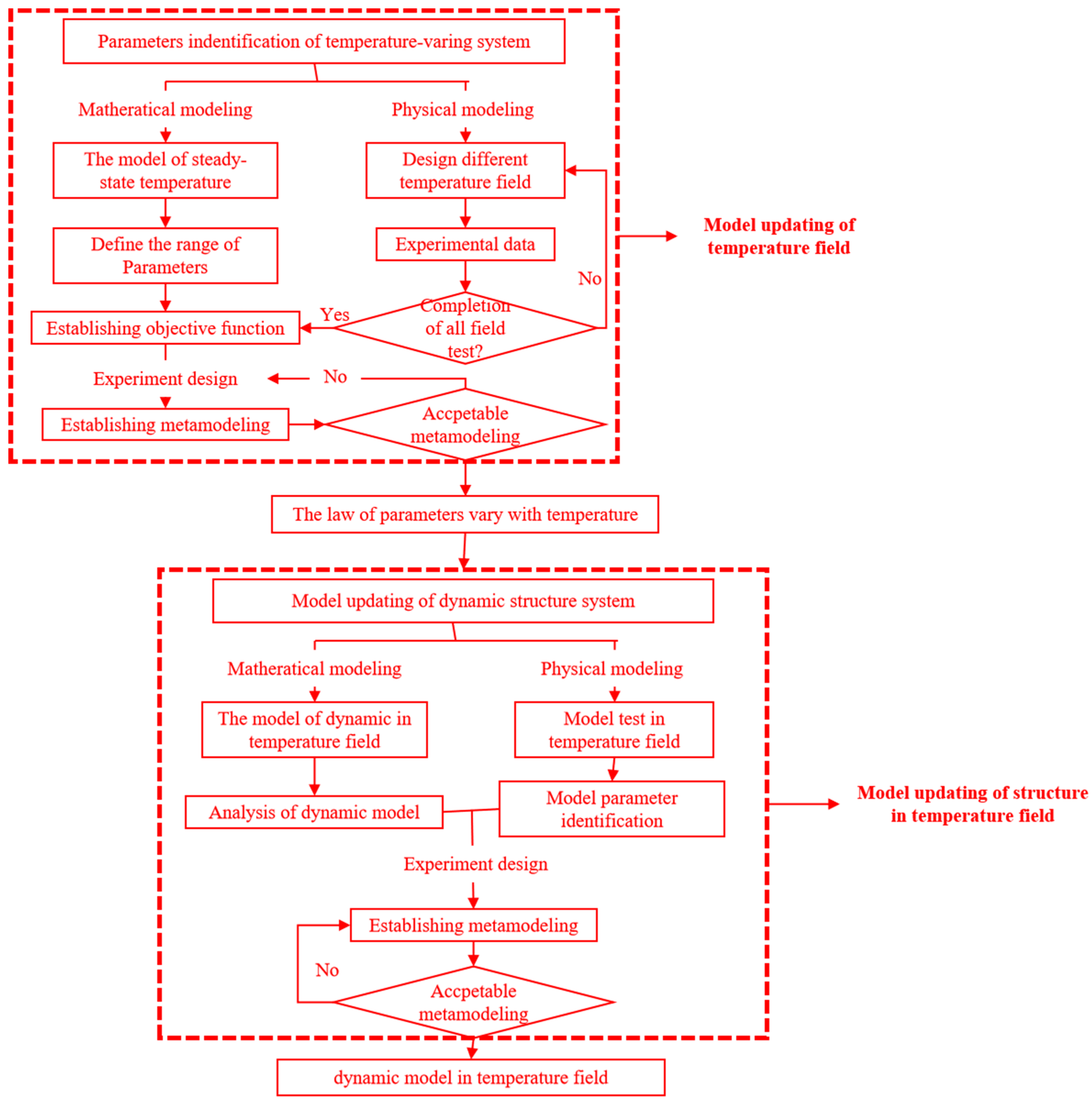
Therefore, a hierarchical correction method is introduced into the updating process of the structural dynamics of finite element model considering the temperature effect, which can be based on the different order of action of the thermal physical and structural dynamics parameters on the structural dynamics’ properties in the thermal environment, with the temperature field correction as the first level correction and the structural dynamics correction as the second level correction. The flow chart of hierarchical correction is shown in Figure 1.

3. Support Vector Regression

3.1. The Theory of Support Vector Regression

The statistical learning theory (also known as support vector regression) proposed by Vapnik [17] is a specialized theory for small samples that avoids the problems of difficult to determine network structure, over-learning, under-learning and local minima that occur with methods such as artificial neural networks. It is considered to be the one of best theories available for solving problems such as classification and regression for small samples [18]

Suppose the sample set is ${\{(x_i,y_i)\}}_{i=1}^N$, where $x_i\in R^n$ represents the input of the sample and $y_i\in R^n$ represents the output of the sample, and SVR can be expressed as the existence function:

$$y=f(x)$$

(8)

The $\epsilon$-insensitive loss function is introduced as follows:

$$L(x_i,y_i)=\{\begin{array}{l}0\hspace{1em}\hspace{1em}\hspace{1em}\hspace{1em}\hspace{1em}, f(x_i)-y_i<\epsilon \\ f(x_i)-y_i-\epsilon ,\hspace{1em}\hspace{1em}\mathrm{else}\end{array}$$

(9)

Considering the existence of the fitting error, the relaxation variables $\xi \ge 0$ and $\xi *\ge 0$ are introduced to improve the generalization performance and the mathematical model of SVR, which includes the relaxation variable, is as follows:

$$\begin{array}{l}\min \frac{1}{2}{\Vert w\Vert }^2+C{\displaystyle \sum _{i=1}^N({\xi }_i+{\xi }_i^{*})}\\ \mathrm{s}.\mathrm{t}.\{\begin{array}{l}{y}_i-(<w,x_i>+b)\le \epsilon +{\xi }_i^{*}\\ (<w,x_i>+b)-y_i\le \epsilon +{\xi }_i\\ {\xi }_i,{\xi }_i^{*}\ge 0,i=1,\cdots ,N\end{array}\end{array}$$

(10)

where w is the optimization objectives, $\epsilon$ is the parameter of the insensitive error function, which is used to quantify the error between the fitted data and the training sample, C is penalty functions and a threshold.

The SVR problem above is generally solved by dual theory, which is transformed into a quadratic programming problem. The Lagrange equation is established as follows:

$$\begin{array}{c}L(w,\xi ,\xi *)=\frac{1}{2}{\Vert w\Vert }^2+C{\displaystyle \sum _{i=1}^n({\xi }_i+{\xi }_i^{*})}-{\displaystyle \sum _{i=1}^n{a}_i(\epsilon +{\xi }_i+y_i-<w,x_i>-b)}\\ -{\displaystyle \sum _{i=1}^n{a}_i^{*}(\epsilon +{\xi }_i^{*}+y_i-<w,x_i>-b)}-{\displaystyle \sum _{i=1}^n(\eta {\xi }_i+\eta *{\xi }_i^{*})}\end{array}$$

(11)

The partial derivatives of the above equation for parameters $w$, $b$, ${\xi }_i$ and ${\xi }_i^{*}$ are zero, and this condition can be substituted into Equation (10) to obtain the dual optimization problem:

$$\begin{array}{l}\min \frac{1}{2}{\displaystyle \sum _{i,j=1}^N(a_i^{*}-a_i)(a_j^{*}-a_j)<x_i,x_j>}+{\displaystyle \sum _{i=1}^N{a}_i(\epsilon -y_i)+{\displaystyle \sum _{i=1}^N{a}_i^{*}(\epsilon +y_i)}}\\ \mathrm{s}.\mathrm{t}.\{\begin{array}{l}{\displaystyle \sum _{i=1}^N(a_i^{*}-a_i)=0}\\ 0\le a_i^{*}\le C,0\le a_i\le C,i=1,\cdots ,N\end{array}\end{array}$$

(12)

According to the KKT condition, the optimization problem in the above equation exists the following equations at the optimal solution.

$$\{\begin{array}{l}{\alpha }_i\left(\epsilon +{\xi }_i+y_i-\left(w\cdot x_i\right)-b\right)=0\\ {\alpha }_i^{*}\left(\epsilon +{\xi }_i^{*}-y_i+\left(w\cdot x_i\right)+b\right)=0\end{array}$$

(13)

In addition:

$$\{\begin{array}{l}(C-\alpha ){\xi }_i=0\\ (C-\alpha *){\xi }_i^{*}=0\end{array}$$

(14)

Assuming ${\mathbf{\alpha }}^{(*)}={\left({\alpha }_1,{\alpha }_1^{*},{\alpha }_2,{\alpha }_2^{*},\cdots ,{\alpha }_l,{\alpha }_l^{*}\right)}^T$ is the solution of Equation (13), If there are components of ${\mathbf{\alpha }}^{(*)}$ that take values between $\left(0,C\right)$, then the threshold $\overline{b}$ for the regression problem can be calculated.

$$\{\begin{array}{ccc}\overline{b}=y_j-\epsilon -{\displaystyle \sum _{i=1}^l\left({\overline{\alpha }}_i^{*}-{\overline{\alpha }}_i\right)\left(x_i\cdot x_j\right)}& ,& 0<{\alpha }_i^{*}<C\\ \overline{b}=y_j+\epsilon -{\displaystyle \sum _{i=1}^l\left({\overline{\alpha }}_i^{*}-{\overline{\alpha }}_i\right)\left(x_i\cdot x_j\right)}& ,& 0<{\alpha }_i<C\end{array}$$

(15)

Then, the regression decision function can be constructed as:

$$f(\mathit{x})={\displaystyle \sum _{i=1}^l\left({\overline{\alpha }}_i^{*}-{\overline{\alpha }}_i\right)x_i}+\overline{b}$$

(16)

If the sample is linearly inseparable, it will fall into an infinite loop when solving the regression problem and cause the problem to be unsolvable. In order to solve the inherently nonlinear regression problem, the generally adopted method is used to introduce a nonlinear mapping φ to map the original sample input space to a high-dimensional feature space, so that the highly nonlinear problem in the sample space can be solved by the linear SVR method in the feature space.

Due to the introduction of the nonlinear mapping $\phi$, x_i can be replaced by φ(x_i) in the feature space F, Equation (12) can be rewritten as:

$$\begin{array}{l}\min \frac{1}{2}{\displaystyle \sum _{i=1}^l{\displaystyle \sum _{i=1}^l\left({\alpha }_i-{\alpha }_i^{*}\right)\left({\alpha }_j-{\alpha }_j^{*}\right)\left(\phi \left(x_i\right)\cdot \phi \left(x_i\right)\right)}}+\epsilon {\displaystyle \sum _{i=1}^l\left({\alpha }_i+{\alpha }_i^{*}\right)}-y_i{\displaystyle \sum _{i=1}^l\left({\alpha }_i-{\alpha }_i^{*}\right)}\\ \mathrm{s}.\mathrm{t}. {\displaystyle \sum _{i=1}^l\left({\alpha }_i-{\alpha }_i^{*}\right)}=0\\ \hspace{1em}\hspace{1em}0\le {\alpha }_i^{(*)}\le C,i=1,2,\cdots ,l\end{array}$$

(17)

To simplify the process of solving the regression problem, a kernel function is introduced and satisfies the following:

$$k(x,x^{\prime })=<\phi (x_i),\phi (x_i)>$$

(18)

Equation (11) can be written as:

$$\min \frac{1}{2}{\displaystyle \sum _{i,j=1}^N(a_i^{*}-a_i)(a_j^{*}-a_j)k(x_i,x_j)}+{\displaystyle \sum _{i=1}^N{a}_i(\epsilon -y_i)+{\displaystyle \sum _{i=1}^N{a}_i^{*}(\epsilon +y_i)}}$$

(19)

Therefore, the SVR problem can be expressed as:

$$f(x)={\displaystyle \sum _{x_i\in SV}^N({\overline{a}}_i^{*}-{\overline{a}}_i)k(x_i,x)}+b$$

(20)

where SV is the range of regression issues.

3.2. The Theory of Improved Support Vector Regression

The selection of the kernel function has a great influence on the generalization ability of SVR. SVR with the quad kernel and Gaussian kernel is suitable for constructing surrogate model problems with strong nonlinear characteristics. If a real function has a low degree of nonlinearity or shows a more significant linear characteristic, considering the influence of $\epsilon$, SVR with these two types of kernel functions will have obvious overfitting. For this problem, SVR with a polynomial kernel function can obtain a better fitting effect. Since the selection of different kernel functions is related to the nonlinear characteristics of the fitting function itself, it is difficult to fit a general function with only a single kernel function. Aiming at this problem, this paper mixes the Gaussian kernel function or quad kernel function with a conventional polynomial kernel function and uses this new hybrid kernel function to improve the traditional SVR model. The improved SVR model is shown below:

$$f(x)={\displaystyle \sum _{i=1}^l({\overline{\alpha }}_i^{*}-{\overline{\alpha }}_i)k({\mathit{x}}_i,\mathit{x})}+{\displaystyle \sum _{j=1}^n{c}_j{p}_j(\mathit{x})}$$

(21)

Since the number of parameters to be calculated is more than the number of equations, the above formula cannot be definitively solved. Therefore, the orthogonality condition is introduced:

$$\left[\begin{array}{cc}K& P\\ P^{\mathrm{T}}& \mathbf{0}\end{array}\right]\left[\begin{array}{c}\mathsf{\alpha }\\ c\end{array}\right]=\left[\begin{array}{c}f\\ 0\end{array}\right]$$

(22)

where the kernel function matrix of the improved support vector regression machine is a nonpositive definite matrix. In the process of constructing the surrogate model of SVR, when quadratic programming is used to solve the optimal coefficients, the kernel function matrix must be a positive definite matrix. Therefore, it is necessary to construct a suitable response function to solve the problem of quadratic programming.

The new response function is defined as:

$$g(x)={(k(x)-f)}^T(k(x)-f)$$

(23)

where k(x) represents the kernel function and f represents the original response value. Therefore, the new secondary planning problem is described as:

$$\min \frac{1}{2}{x}^T{k}^{T}kx+x^T(k^{T}f)$$

(24)

Choosing the sample space. A suitable DOE is the key to sampling and determines the sample quantity and spatial distribution for constructing surrogate models. The normal DOE methods include the full factorial design of the experiment, central composite design of the experiment, orthogonal experimental design, uniform design of the experiment, random bit design and Latin square method. In this paper, the full factorial design of the experiment and central composite design of the experimental methods are used for sampling.

Building the appropriate set of sample points based on the inputs and outputs and using a suitable experimental design method. The accuracy of the constructed surrogate model needs to be verified and ANOVA is a common method of verification. In this manuscript, the coefficient of determination $R^2$ and the RMSE are introduced to examine the model precision:

$$R^2=1-SSE/SST$$

(25)

$$RMSE=\frac{\sqrt{SSE}}{n\cdot \overline{f}}$$

(26)

where n represents the number of nonconstant in the surrogate model. Generally, there is a negative correlation between $R^2$ and RMSE; additionally, there is a positive correlation between $R^2$ and the model adaptability. SSE represents the error sum of squares, SST represents the total error sum of squares and the functions of SSE and SST are shown in the following:

$$SSE={\displaystyle \sum _{i=1}^n{(f_i-f_i^{\prime })}^2}$$

(27)

$$SST={\displaystyle \sum _{i=1}^n{(f_i-\overline{f})}^2}$$

(28)

where $f_i$ is the real response value of the sample point space, $f_i^{\prime }$ is the calculation response value of the surrogate model of the sample point space and $\overline{f}$ is the average value of the real response value and calculation response value of the sample point space.

4. Thermophysical Parameters Identification

At present, is it common for methods to assume that modified thermophysical parameters are constants or known function forms. However, the variation in thermophysical parameters with temperature dependence is much more complicated in practical engineering. In this paper, a set of linear combinations of basis functions is used to define the function of thermophysical parameters in a temperature-dependent manner, in which the basis functions can be expressed by SVR:

$$k_j={\displaystyle \sum _{i=0}^{N_T}{\alpha }_{j,i}{\psi }_{j,i}(T) j=1,\cdots ,s}$$

(29)

where $s$ is the number of thermophysical parameters, ${\psi }_i$ is the basis function and ${\alpha }_i$ is the coefficient of the basis function. Then, the thermophysical parameters can be defined as the optimization variables, and the residual error between the experimentally measured datum and the datum calculated during simulations can be defined as the objective function; the objective function can be minimized to obtain the optimal results.

$$J={\displaystyle \sum _{i=1}^n\left|T_i^a(k)-T_i^t\right|}$$

(30)

where $k$ is the thermophysical parameter vector, $n$ is the number of temperature measuring points, and $T_i^a$ and $T_i^t$ are the $i$th simulation calculated datum and experimentally measured datum, respectively.

Then, the thermophysical parameter identification problem is solved as an optimization problem; that is, the thermophysical parameters are defined as a temperature-dependent function, which satisfies the following:

$$\mathbf{K}=\mathbf{Q}\mathbf{T}$$

(31)

where $K$ is the thermophysical parameter matrix, $T$ is the temperature matrix and $Q$ is the coefficient matrix.

According to the coefficient matrix identification model, which is used to minimize the residual error between the experimentally measured datum and simulation calculated datum, the surrogate model is used for further calculation. The flow chart of thermophysical parameter identification with temperature dependence is shown in Figure 2.

5. The Numerical Examples

5.1. A Numerical Example of Two Parameters

According to a nonlinear function named Branin rcos, the precision of the global approximate function constructed by SVR-Polynomial, SVR-Gauss and improved SVR based on the hybrid basis function (improved SVR) are compared. There are two variables in this function:

$$f(x)={(x_2-\frac{5.1x_1^2}{4{\pi }^2}+\frac{5x_1}{\pi }-6)}^2+10(1-\frac{1}{8\pi })\cos (x_1)+10$$

(32)

where $x_1\in [-5,10]$ and $x_2\in [0,15]$.

The full factorial DOE is used to solve the above small-scale problem, which defines the normalized parameters x₁ and x₂ as ${\overline{x}}_1$ and ${\overline{x}}_2$. The sample points and objective function values are shown in

Table 1. The full factorial experimental design based on 2 level.

Number	x1	x2	$\mathit{f}$	Number	x1	x2	$\mathit{f}$
1	−1	−1	308.1	14	0	0.5	60.57
2	−1	−0.5	80.12	15	0	1	22.17
3	−1	0	10.31	16	0.5	−1	47.98
4	−1	0.5	20.8	17	0.5	−0.5	22.38
5	−1	1	10.96	18	0.5	0	73.23
6	−0.5	−1	193.3	19	0.5	0.5	122.6
7	−0.5	−0.5	32.75	20	0.5	1	69.96
8	−0.5	0	3.156	21	1	−1	17.51
9	−0.5	0.5	26.62	22	1	−0.5	59.39
10	−0.5	1	2.501	23	1	0	150.5
11	0	−1	106.6	24	1	0.5	212.8
12	0	−0.5	13.51	25	1	1	145.9
13	0	0	24.13

.

The surrogate models using SVR based on different basis functions and the real function are shown in Figure 3, the number of sample points is 1600.

From the figures above, we can find that SVR based on different basis functions can fit the real function according to the sample points. The difference is that the fitting results and accuracy of the constructor function based on SVR-Polynomial are the poorest and have severe overfitting phenomena. Even though the constructor function based on SVR-Gauss can describe the real function more accurately to some degree, from Figure 3c, we can find that there is obvious deviation between the constructor function and real function in some areas. However, the constructor function based on improved SVR can exactly describe the real function, so its accuracy is the highest. To illustrate it more directly, we apply the method of comprehensive factorial experimental design to create a series of test samples to test the accuracy of the constructor function.

To further prove that the surrogate model based on improved SVR has the best fitting precision, a group of test sample points was constructed through the full factorial DOE method and the test sample points are listed in

Table 2. The test sample points.

Number	x1	x2	Number	x1	x2
1	−0.7	−0.7	9	0.3	−0.7
2	−0.7	−0.3	10	0.3	−0.3
3	−0.7	0.3	11	0.3	0.3
4	−0.7	0.7	12	0.3	0.7
5	−0.3	−0.7	13	0.7	−0.7
6	−0.3	−0.3	14	0.7	−0.3
7	−0.3	0.3	15	0.7	0.3
8	−0.3	0.7	16	0.7	0.7

.

According to Equations (27) and (28), R² and RMSE can be obtained.

Table 3. The R² and RMSE.

	R2	RMSE
SVR-Polynomial	0.7374	0.0869
SVR-Gauss	0.8768	0.0184
Improved SVR	0.9995	0.0052

shows that the R² value of the surrogate model based on improved SVR is larger than that based on SVR-Quad and SVR-Gauss, and the RMSE value of the surrogate model based on improved SVR is less than that based on SVR-Polynomial and SVR-Gauss. This means that among these three surrogate model construction methods, improved SVR obtains the best fitting precision and a more accurate description.

5.2. Thermophysical Parameters Identification of Aluminum Alloy Plate

This numerical example shows the general process of identifying the thermophysical parameters, which vary with the temperature of some aluminum alloy plates according to the heat transfer coefficient, with temperature dependence based on SVR. The aluminum alloy plate has a size of $2\times 0.6\times 0.004$ m, there are 750 quadrilateral shell elements in the finite element mode. In order to verify the accuracy of the thermal parameter identification method, we define the thermal boundary conditions as a heating temperature upper bound of 300 °C, and an ambient temperature of 20 °C, which is conducted from the short side of one end of the aluminum sheet to the other. To facilitate the calculation and comparison, the following assumptions are made:

(1)

Assume that the real heat transfer coefficients satisfy the distribution in

Table 4. The real heat transfer coefficients distribution.

Temperature/°C	$\mathbf{Heat} \mathbf{Transfer} \mathbf{Coefficients}/(\mathbf{W}/({\mathbf{m}}^2·°\mathrm{C}))$
20	237
125	246
175	268
250	304
300	330

.

(2)

The emissivity of thermal radiation has been identified in previous work [19] is 0.09 in this study.

(3)

The influence of the screw thermal contract on the temperature distribution is ignored.

Table 5. The upper and lower boundaries of modified thermophysical parameters.

	Low Temperature/20 °C	High Temperature/300 °C
Upper $(\mathrm{W}/({\mathrm{m}}^2·°\mathrm{C}))$	220	320
Lower $(\mathrm{W}/({\mathrm{m}}^2·°\mathrm{C}))$	250	350

shows the design space of the upper and lower boundaries of the modified thermophysical parameters.

The Figure 4 shows that the real temperature distribution, the initial temperature distribution and the updated temperature distribution are generally consistent according to the comparison above. However, there is a dislocation in the position on the aluminum alloy plate when comparing the initial temperature distribution in the range of 200–80 °C with the real temperature distribution, and the updated temperature distribution and the real temperature distribution are almost the same. To further illustrate the consistency between the real temperature distribution and the updated temperature distribution based on the thermophysical parameter identification method proposed in this paper, seven typical nodes are selected in the finite element model to analyze the deviations among the real temperature, initial temperature and updated temperature.

Table 6. The comparison among real temperature, initial temperature and updated temperature.

Nodes Number	Real Temperature (°C)	Initial Temperature (°C)	Deviation	Updated Temperature (°C)	Deviation
32	288.45	286.00	0.85%	288.41	0.013%
86	258.61	251.25	2.85%	258.52	0.035%
151	220.74	209.00	5.32%	220.67	0.032%
216	180.32	167.00	7.39%	180.37	0.028%
281	136.89	125.00	8.69%	136.96	0.051%
346	90.78	83.00	8.57%	90.97	0.21%
411	43.79	41.00	6.37%	43.80	0.23%

shows the deviation comparisons.

It is shown in Table 6 that the deviation in the initial temperature distribution and the real temperature distribution is small in the high temperature range, and the deviation gradually increases as the temperature decreases. The deviation between the updated temperature distribution and the real temperature distribution is almost negligible in each temperature range. Therefore, the thermophysical parameter identification method proposed in this paper can obtain a consistent temperature distribution with the real distribution.

Assuming that the variation in the heat transfer coefficient with temperature dependence satisfies a higher-order polynomial form, which is shown in Figure 5, the simulation result indicates that the method proposed in this paper has higher accuracy than the traditional parametric model updating method. According to the fitting results obtained in MATLAB, the variation in the real heat transfer coefficient with temperature dependence basically satisfies the cubic polynomial, which has the following function form:

$$y=(-5.0553e-6)t^3+0.0036t^2-0.3363t+242.242$$

(33)

Table 7. The range of design space of identified parameters.

Coefficient	Cubic Order	Polynomial Order	First Order	Constant
Upper	−4 × 10−6	0.003	−0.3	230
Lower	−6 × 10−6	0.004	−0.4	250

shows the design space of identified parameters.

Table 8. Comparison of temperature distribution based on the two methods.

Node Number	Real Values (°C)	Parametric (°C)	Deviation	Functional (°C)	Deviation
32	288.45	288.53	0.028%	288.41	0.013%
86	258.61	258.70	0.035%	258.52	0.035%
151	220.74	220.53	0.095%	220.67	0.032%
216	180.32	179.72	0.333%	180.37	0.028%
281	136.89	136.34	0.402%	136.96	0.051%
346	90.78	90.74	0.044%	90.97	0.21%
411	43.79	43.83	0.091%	43.80	0.23%

shows the comparison results of temperature distributions based on parametric updating method and functional updating method.

Table 8 shows that the accuracy of the identification temperature based on the functional updating method of nodes 32, 86, 151, 216 and 281 is higher than the accuracy based on the parametric updating method, while the accuracy of the identification temperature based on the functional updating method of nodes 346 and 411 is lower than the accuracy based on the parametric updating method. In general, the identification results based on the functional updating method have higher precision. Figure 6 shows the comparison histogram of the identification temperature deviations obtained by the two methods above.

5.3. The Thermophysical Parameters Identification of Wing Structure

In this numerical example, a wing structure dynamical modal updating problem with temperature dependence is presented to verify the method proposed in this paper; the finite element model is shown in Figure 7.

The wing chord length is 0.595 m, half span chord ratio is 2.81, wing thickness ratio is 0.12. There are 5446 quadrilateral shell elements in the finite element model of wing structure, and wing root is restrained by means of fixed restraints. According to the principle of hierarchical model updating, the temperature field is first applied to the finite element model to generate temperature stresses. Then, the temperature stresses are added to the model as pre-stresses for modal frequency analysis.

This numerical example is only used to verify the accuracy of the identification method, and some assumptions are made to complete the calculation.

(1)

The wing structure material is aluminum alloy with a density of, 2800 kg/m³, Poisson’s ratio is 0.33, heat transfer coefficient is shown in the Table 1 and temperature-dependent elastic modulus is shown in

Table 9. The real elastic modulus with temperature-dependent.

Temperature/°C	Elastic Modulus/GPa
20	70
100	69
150	67
200	61
250	56
300	48

.

(2)

The finite element model has been simplified, and the influences of rivets, bolts and other parts of the thermal contact with temperature-dependent to temperature distribution have been ignored.

5.3.1. The Temperature Distribution Model Updating

The temperature distribution is determined by material thermophysical parameters, the influence of the structural installation is ignored, and the external heating conditions are determined. In this numerical simulation, the heat transfer coefficient is identified with the method above, and the real temperature distribution, initial temperature distribution and identified temperature distribution are shown in Figure 8.

There are 20 nodes selected in the finite element model, they are used to compare the deviations in the real temperature, initial temperature and identified temperature, and the results are shown in

Table 10. The comparison of real temperature, initial temperature and identified temperature.

Node Number	Real Temperature (°C)	Initial Temperature (°C)	Deviation	Identified Temperature (°C)	Deviation
118	52.15	48.42	7.15%	52.17	0.038%
565	77.64	71.18	8.32%	77.71	0.090%
1108	117.35	107.06	8.77%	117.63	0.239%
1928	142.49	130.25	8.59%	142.59	0.070%
2542	168.74	155.50	7.85%	168.78	0.024%
3006	201.83	188.99	6.36%	201.76	0.035%
3633	223.14	211.60	5.17%	223.03	0.049%
4108	254.30	246.09	3.23%	254.18	0.047%
4522	280.70	276.75	1.41%	280.64	0.021%
4605	252.63	244.20	3.34%	252.51	0.048%
4624	160.11	147.07	8.14%	160.17	0.037%
4715	133.59	121.94	8.72%	133.74	0.112%
4722	192.10	178.96	6.84%	192.07	0.016%
4740	270.89	265.20	2.10%	270.80	0.033%

.

Table 10 shows that the deviation between the real temperature and identified temperature is very small, and the maximum deviation is less than two thousandths. The results show that the temperature distribution is highly reliable and can be used in subsequent updating calculations.

5.3.2. Structural Dynamic Modal Updating

A structural dynamic model with temperature dependence is presented when the identified temperature distribution is loaded. Assuming the elastic modulus is the only source of model error, the influences of other parameters are not considered. The range of the identified elastic modulus with temperature dependence is shown in Figure 9.

Due to the large size of the model and the complexity of the structure, it would be time-consuming to use a direct finite element model for modal frequency analysis considering pre-stress, so a surrogate model is used instead of a finite element model for calculations, the number of sample points is 2500.

The natural frequency calculated with the given elastic modulus is taken as the experimentally measured datum. The comparison of the first four orders of natural frequencies about the real natural frequency, initial natural frequency and updated natural frequency is shown in

Table 11. The range of elastic modulus with temperature-dependent.

	Low Temperature/20 °C	High Temperature/300 °C
Upper/GPa	60	40
Lower/GPa	80	50

, and the first four orders of mode shapes are shown in Figure 9.

In

Table 12. The comparison of real natural frequency, initial natural frequency and updated natural frequency.

Order	Real Natural Frequency (Hz)	Initial Natural Frequency (Hz)	Deviation	Updated Natural Frequency (Hz)	Deviation
First	22.81	24.454	7.21%	22.98	0.75%
Second	110.17	117.32	6.49%	110.94	0.70%
Third	114.32	122.63	7.27%	115.59	1.11%
Forth	140.05	151.32	8.05%	141.53	1.06%

and Figure 9, it is obvious that the deviation between the real natural frequency and initial natural frequency of the first three bending modes and the first tensional mode is 6−8%, and the deviation between the real natural frequency and updated natural frequency is only 1%. This illustrates that a thermal structural dynamic model with high precision can be obtained by thermophysical parameter identification and the dynamic modal updating method proposed in this paper.

6. Conclusions

In this paper, a structural dynamic model updating method with thermal effects based on improved SVR is proposed. Assuming the thermophysical parameters are linear combinations of basis functions, which can be expressed by improved SVR, the numerical simulation results show the following conclusions:

(1)

The functional updating method has a wider use range, higher precision and clearer physical meaning than the traditional matrix updating method and parametric updating method.

(2)

It obtains a reliable temperature distribution model according to the identification method with temperature dependence proposed in this paper.

(3)

The hierarchical correction method is introduced to modify the temperature distribution model and structural dynamic model and effectively solves the model updating problem in a temperature-dependent manner. Therefore, the temperature-dependent model updating method can be applied to practical complex heat transfer processes, which is beneficial to practical applications.

References

1. Wang, C.C.; Yang, C.Y. Inverse method in simultaneously estimate internal heat generation and root temperature of the T-shaped fin. Int. Commun. Heat Mass Transf. 2010, 37, 1312–1320. [Google Scholar] [CrossRef]
2. Tsai, C.H.; Young, D.L.; Kolibal, J. Numerical solution of three-dimensional backward heat conduction problems by the time evolution method of fundamental solutions. Int. J. Heat Mass Transf. 2011, 54, 2446–2458. [Google Scholar] [CrossRef]
3. Lu, T.; Liu, B.; Jiang, P.X. Inverse estimation of the inner wall temperature fluctuations in a pipe elbow. Appl. Therm. Eng. 2011, 31, 1976–1982. [Google Scholar] [CrossRef]
4. Sawaf, B.; Özisik, M.N. Determining the constant thermal conductivities of orthotropic materials by inverse analysis. Int. Commun. Heat Mass Transf. 1995, 22, 201–211. [Google Scholar] [CrossRef]
5. Huang, C.H.; Wang, S.P. A three-dimensional inverse heat conduction problem in estimating surface heat flux by conjugate gradient method. Int. J. Heat Mass Transf. 1999, 42, 3387–3403. [Google Scholar] [CrossRef]
6. Gosselin, L.; Tye-Gingras, M.; Mathieu-Potvin, F. Review of utilization of genetic algorithms in heat transfer problems. Int. J. Heat Mass Transf. 2009, 52, 2169–2188. [Google Scholar] [CrossRef]
7. Sahoo, N.; Peetala, R.K. Transient temperature data analysis for a supersonic flight test. J. Heat Transf. 2010, 132, 084503. [Google Scholar] [CrossRef]
8. Wang, J.; Zabaras, N. Using Bayesian statistics in the estimation of heat source in radiation. Int. J. Heat Mass Transf. 2005, 48, 15–29. [Google Scholar] [CrossRef]
9. Cui, M.; Gao, X.; Zhang, J. A new approach for the estimation of temperature-dependent thermal properties by solving transient inverse heat conduction problems. Int. J. Therm. Sci. 2012, 58, 113–119. [Google Scholar] [CrossRef]
10. Cappelli, L.; Montemurro, M.; Dau, F.; Guillaumat, L. Characterisation of composite elastic properties by means of a multi-scale two-level inverse approach. Compos. Struct. 2018, 204, 767–777. [Google Scholar] [CrossRef] [Green Version]
11. Cappelli, L.; Montemurro, M.; Dau, F.; Guillaumat, L. Multiscale Identification of Material Properties for Anisotropic Media: A General Inverse Approach. In Advances in Predictive Models and Methodologies for Numerically Efficient Linear and Nonlinear Analysis of Composites; Springer: Cham, Switzerland, 2019. [Google Scholar]
12. Cappelli, L.; Montemurro, M.; Dau, F.; Guillaumat, L. Multi-scale identification of the viscoelastic behaviour of composite materials through a non-destructive test. Mech. Mater. 2019, 137, 103137.1–103137.14. [Google Scholar] [CrossRef]
13. Cappelli, L.; Balokas, G.; Montemurro, M.; Dau, F.; Guillaumat, L. Multi-scale identification of the elastic properties variability for composite materials through a hybrid optimisation strategy. Composites 2019, 176, 107193.1–107193.12. [Google Scholar] [CrossRef]
14. Montemurro, M.; Nasser, H.; Koutsawa, Y.; Belouettar, S.; Vincenti, A.; Vannucci, P. Identification of electromechanical properties of piezoelectric structures through evolutionary optimisation techniques. Int. J. Solids Struct. 2012, 49, 1884–1892. [Google Scholar] [CrossRef]
15. Audoux, Y.; Montemurro, M.; Pailhès, J. Non-Uniform Rational Basis Spline hyper-surfaces for metamodelling. Comput. Methods Appl. Mech. Eng. 2020, 364, 112918. [Google Scholar] [CrossRef]
16. Audoux, Y.; Montemurro, M.; Pailhès, J. A Metamodel Based on Non-Uniform Rational Basis Spline Hyper-Surfaces for Optimisation of Composite Structures. Compos. Struct. 2020, 247, 112439. [Google Scholar] [CrossRef]
17. Vapink, V. Statistical Learning Theory; Wiley: New York, NY, USA, 1998. [Google Scholar] [CrossRef]
18. Clarke, S.M.; Griebsch, J.H.; Simpson, T.W. Analysis of support vector regression for approximation of complex engineering analyses. J. Mech. Des. 2005, 127, 1077–1087. [Google Scholar] [CrossRef]
19. Zuo, Y.P. Research on IR-Emissivity of 2A12 and TC4 Alloy in Different Microstructure and Surface States. Master’s Thesis, Nanjing University of Aeronautics and Astronautics, Nanjing, China, 2008. [Google Scholar]
Figure 1. The flow chart of hierarchical correction.
Applsci 11 08025 g001
Figure 2. Flow chart of thermophysical parameter identification with temperature dependence.
Applsci 11 08025 g002
Figure 3. The contraction based on different basis function.
Applsci 11 08025 g003
Figure 4. The comparison between real temperature distribution, initial temperature distribution and updated temperature distribution.
Applsci 11 08025 g004
Figure 5. The cubic polynomial fitting curve of real heat transfer coefficient.
Applsci 11 08025 g005
Figure 6. Comparison of identification temperature deviations based on the two methods.
Applsci 11 08025 g006
Figure 7. The finite element model of wing structure.
Applsci 11 08025 g007
Figure 8. The comparison of real temperature distribution, initial temperature distribution and updated temperature distribution.
Applsci 11 08025 g008
Figure 9. Mode shapes of the first four orders.
Applsci 11 08025 g009