Abstract
Vehicle interior noise is an important factor affecting ride comfort. To reduce the noise inside the vehicle at the vehicle body design stage, a finite element model of the vehicle body must be established. While taking the first-order global modal of the body-in-white, the maximum sound pressure level of the target point in the vehicle, the body mass, and the side impact conditions into account, the thickness of the body panel as determined via sensitivity analysis is treated as the input variable, and the sample is determined by following the Hamersley experimental design. Specifically, the Elman neural network predicts the noise value in the vehicle, and a vehicle body structure optimization method that comprehensively considers NVH performance and side impact safety is established. The prediction errors of the Elman neural network algorithm were within 3%, which meets the prediction accuracy requirements. To achieve satisfactory restraint performance, the maximum sound pressure level of the target point in the vehicle is reduced by 5.92 dB, and the maximum intrusions of the two points on the B-pillar inner panel are reduced by 31.1 mm and 33.71 mm, respectively. The side impact performance is improved while the noise inside the vehicle is reduced. This study provides a reference method for multidisciplinary research aiming to optimize the design of vehicle body structures.
1. Introduction
The noise, vibration, harshness (NVH) performance of a vehicle is an important design index in the R&D stage that has attracted much attention from users [1,2]. Accordingly, how to improve the acoustic environment of the vehicle passenger compartment, reduce the noise level, and improve the NVH performance has become a hot spot in automotive research [3]. When the engine is working, inertial excitation and unbalanced force are generated, hence vibrating the body panels and radiating low- and medium-frequency structural noise to the cabin. Traditional acoustic packages, such as sound absorption and insulation, are mainly aimed at mid- and high-frequency air noise yet have minimal effects on reducing mid- and low-frequency structural noise [4]. Therefore, reducing the mid- and low-frequency structure noise caused by engine excitation is an important research topic in automotive NVH. According to its noise generation mechanism, reducing structure noise in a vehicle to a satisfactory level usually requires modifications in the main parameters of the vehicle body structure.
Many scholars have examined the optimization of vehicle interior noise. For instance, Bao et al. [5] proposed a far-field acoustic hologram that applies a new sound source identification and low-noise technology to guide the optimal design of low-frequency noise in automobiles. Chen et al. [6] established a statistical energy analysis model for commercial cabs and used the NSGA II algorithm along with the weighting coefficient method to optimize the acoustic package parameters. Huang et al. [7] used continuous wavelet transform and coherent analysis to identify the frequency band of internal noise and the contribution of structural noise to the noise inside a vehicle. Liao et al. [8] used a composite noise reduction material with damping and sound absorption functions to control the noise inside a vehicle and found that this approach significantly improved the noise level in a hybrid vehicle. Wu et al. [9] used the source-path-receiver model to identify the path that causes roaring inside a vehicle and then changed the mechanical structure of the vehicle to reduce noise. Lee et al. [10] performed a statistical energy analysis to predict the noise inside a vehicle and found that the predicted sound pressure level was in good agreement with the measured value. Huang et al. [11] performed an interval analysis to identify the source of structural noise of electric vehicle suspension, optimized the component parameters, and improved the noise quality inside a vehicle.
The above studies have used real vehicles as their research objects. Given that NVH optimization needs to be performed at the trial production or mass production stage and that iterative testing should be conducted after optimizing the parts, the entire NVH optimization process is very complex and consumes much time.
At the vehicle body design stage, a vehicle body acoustic-structure coupling finite element model is established, the finite element model is analyzed, and problems in the design of the vehicle body structure are identified in advance. By modifying the body structure parameters to reduce vehicle interior noise, the NVH optimization time of the vehicle during the design phase and the subsequent trial production and mass production phases can be greatly minimized. Previous studies have recognized and reduced vehicle interior noise based on the finite element model of the vehicle body [12,13,14,15,16,17,18]. Kim et al. [19] used the progressive quadratic response surface method to optimize the lower arm of the vehicle suspension system. Zhang et al. [20] established an approximate model from the thickness of the key panel to the peak noise at the driver’s right ear based on the basis function and used the genetic algorithm to solve the optimization model, which reduced the sound pressure level of the key frequency. Chen et al. [21] used the response surface method to establish a connection between the gear lead crown and involute modifications of the 3rd-gear pair to the transmission radiation noise. By optimizing the response surface, the transmission measurement noise at the measuring point was reduced by 2 dB to 4 dB (A). Given the large finite element model of the vehicle, the finite element calculation process consumes a large amount of resources. To reduce the amount of calculation, the abovementioned NVH optimization study based on the finite element model applies the response surface methodology and other approximate models instead of undergoing the calculation process. However, the establishment of the response surface approximation model has high requirements for the designed experimental points. If these experimental points are not properly selected, then the accuracy of the response surface will be greatly reduced.
Neural networks can approximate any nonlinear process [22] and have been recently applied in predicting and optimizing automobile noise given their high prediction accuracy [23,24,25]. Wang et al. [26] proposed a finite element neural network model to simulate the acoustic behavior of the auditory system. Zhang et al. [27] demonstrated the feasibility for the neural network to optimize noise in a vehicle through the error of the neural network prediction and boundary element calculation values. Peng et al. [28] used a BP neural network model to predict the acoustic response characteristics of commercial cabs. Qian et al. [29] proposed a GA-BP-based electric vehicle sound quality prediction model, which offers many advantages in accuracy and generalizability. The neural network compensates for the shortcomings of the traditional response surface prediction model that is overly dependent on experimental points. Therefore, the neural network is selected in this article as the basic model for vehicle interior noise prediction. Although some achievements have been reported in the use of neural networks to predict vehicle noise, the accuracy of this approach needs to be improved, and the appropriate neural network algorithm needs to be identified. Liang et al. [30] used the Elman neural network to accurately predict short-term temperature changes in a digester. Li et al. [31] used the same network to predict the battery capacity of electric vehicles in real time. Abdelhafez et al. [32] used three neural networks to predict active COVID-19 cases in Jordan. In these applications, the Elman model demonstrated its high predictive ability and a significantly better prediction accuracy compared with NARX and feed forward networks. Li et al. [33] predicted indoor temperature using the Elman neural network algorithm and found that this algorithm has a simple structure, small storage space, and high prediction accuracy. Guo et al. [34] designed an Elman neural network predictive controller to solve the nonlinearity of the electro-hydraulic compound steering system of heavy commercial vehicles. Inspired by these achievements, this article uses the Elman neural network to predict the noise inside a vehicle and compares its prediction accuracy with that of other neural network algorithms.
The structural noise in a vehicle is mainly radiated from body panel vibration. In this paper, all panels surrounding the acoustic cavity in a vehicle are treated as design variables, and an optimal combination of variables that meets the specified conditions is selected. The B-pillar inner panel, side wall, roof, and other panels are coupled with the interior acoustic cavity given their significant impact on interior noise. The changes in the thickness of some panels due to NVH optimization can greatly affect the side impact performance [35,36,37]. In the abovementioned research, when optimizing structural parameters such as the thickness of body panels, only the characteristics of the lightweight body and body-in-white modal are considered. However, the important influence of the adjusting these structural parameters on the safety performance of the vehicle body has been largely ignored.
This article takes a minicar as an example. The side impact performance of this vehicle is considered while optimizing its NVH. The maximum intrusion of the B-pillar inner panel of the side impact, the first-order global modal of the body-in-white, and the body mass are all treated as constraints, and the A-weighted sound pressure level at the ear is treated as the target. A multidisciplinary optimization design method that uses the Elman neural network algorithm to comprehensively consider vehicle NVH and collision safety is then explored.
2. Establish a Finite Element Model
2.1. Vehicle Body Finite Element Model
In Hypermesh, 8 mm 2D units are used to mesh the body-in-white, front cover, and other components of the vehicle. The doors and other closures are connected to the vehicle body through the rigid unit, and the adhesives unit is used to simulate the connection of the glass to the vehicle body and door. The location of the solder joints is determined by the point file. The total number of solder joints is 7341, including 4497 bars and 2862 weld units. The total number of vehicle units is 844,388, of which the triangular unit accounts for 5.9% (49,829), which meets the accuracy requirements. The model is shown in Figure 1.
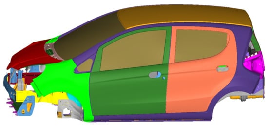
Figure 1.
Vehicle body finite element model.
2.2. Acoustic-Structure Coupling Model
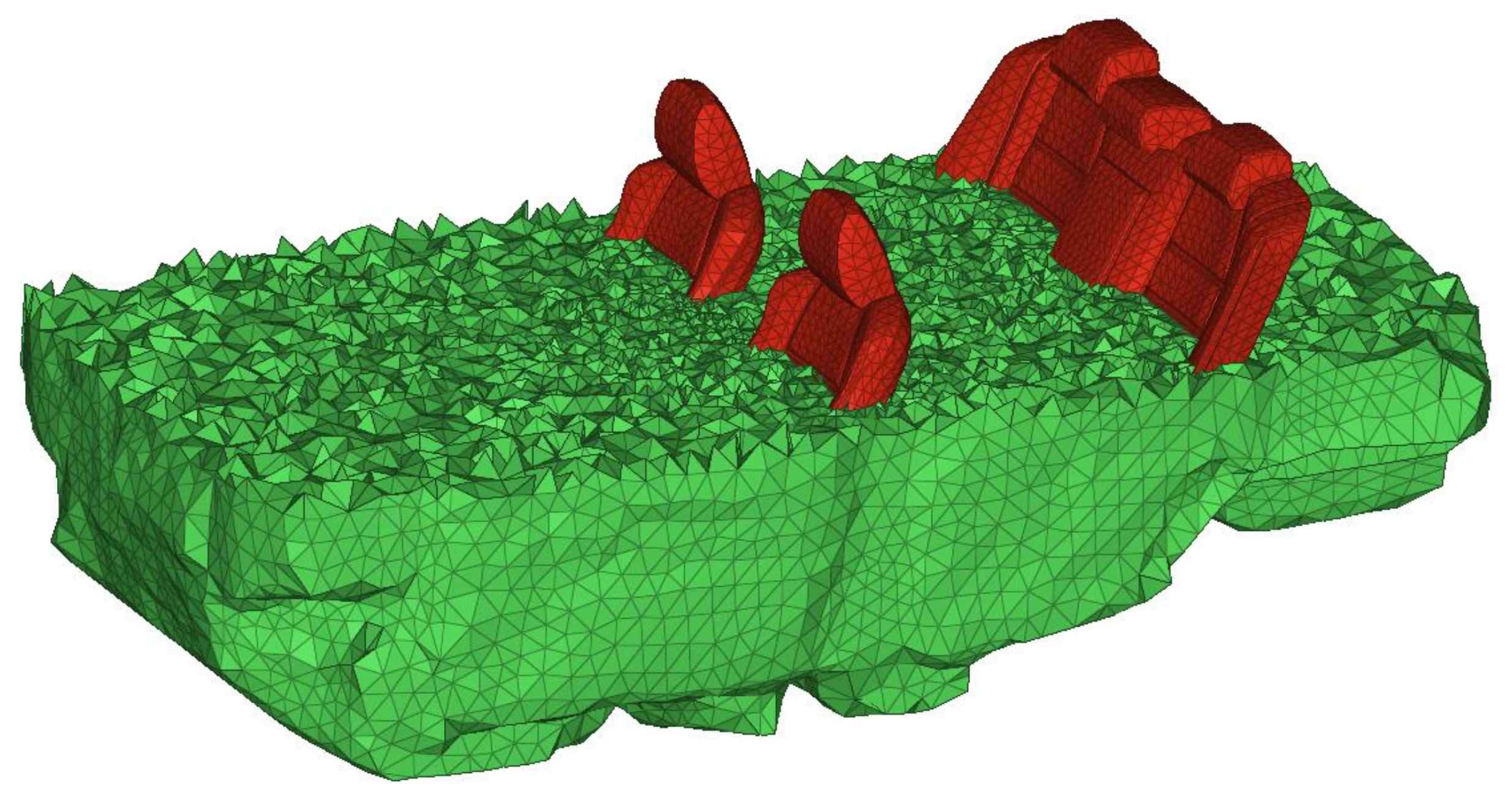
Establishing an acoustic cavity grid requires an airtight vehicle body and a small hole in the vehicle body. In this article, the low-frequency noise within 200 Hz is studied. Given that f = 400 Hz according to the sampling theorem, the minimum wavelength is set to 0.85 m. With 12 cells per wavelength, the cell length is measured as 71 mm, and combined with the calculation accuracy requirements, the side length of the tetrahedral grid is set to 60 mm. An acoustic cavity grid is established with a seat considering the sound absorption characteristics of the latter. The seat and acoustic cavity share common nodes. The acoustic cavity model section is shown in Figure 2. ACMODL cards are used to establish a coupling model in a node-to-node manner.
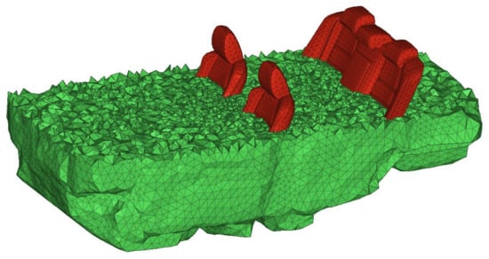
Figure 2.
Sectional view of acoustic cavity model.
2.3. Modal Analysis
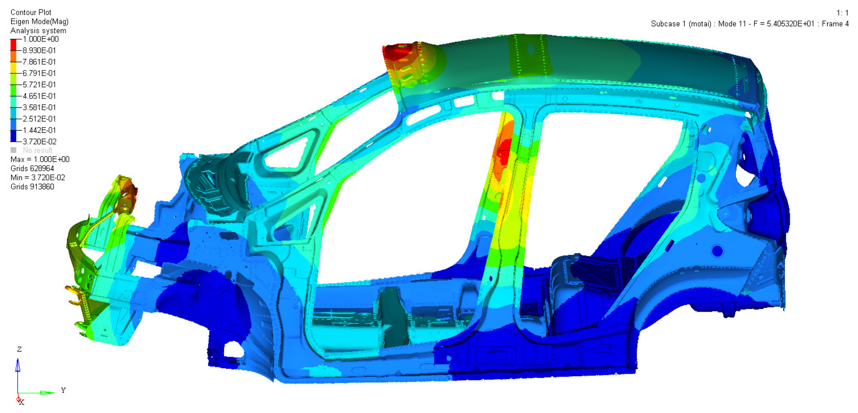
In the automotive NVH performance design and optimization, the first-order global modal data must be fully considered because of the low first-order modal frequency value, which is easily excited by external excitations such as those in the engine and on the road surface, thereby leading to vehicle body resonance. Given that the first-order global modal acts as the overall modal of the vehicle body, the accessory parts of the vehicle body will vibrate at the occurrence of resonance. Moreover, the collision and friction among vehicle parts not only generate noise but also generate fatigue. Therefore, in the optimization process, the first-order global modal of the body-in-white should not be reduced. The modal solution file is submitted to the Optistruct calculation. The first-order global modal shapes are shown in Figure 3 and Figure 4. Some modal frequencies and vibration shapes are shown in Table 1. In addition, the modals of the body including the doors and windows are calculated to observe the modal shapes and frequencies of the doors and windows. The modal shape of front windshield is shown in Figure 5, and the modal shapes and frequencies of doors and windows are shown in Table 2. It can be seen from Table 2, the local modal frequencies of the doors and windows are relatively high and are not easily aroused by external excitations such as the engine. The first-order torsion modal frequency and the first-order bending modal frequency of the body-in-white are determined as the optimization constraints.
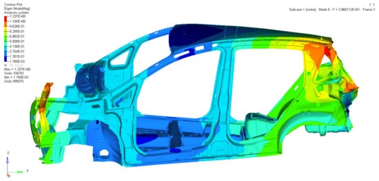
Figure 3.
The first-order torsional modal shape of the body-in-white.

Figure 4.
The first-order bending modal shape of the body-in-white.

Table 1.
The first eight modal frequencies and vibration shapes of the body-in-white.
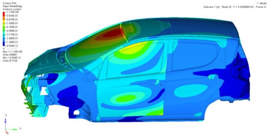
Figure 5.
Modal shape of front windshield.
Table 2.
Modal shapes and frequencies of doors and windows.
When the modal frequencies of the body finite element model are within a reasonable range, the finite element model can be closer to the actual vehicle structure, and the calculation results can better simulate the vibration characteristics of the vehicle structure. Guo et al. [12] compared the modal frequencies of the experimental model and the finite element model, and the errors are all within 10%. Among the modal frequencies of the experimental model, the first-order modal frequency is 24.6 Hz, and the local modal frequency of the roof is 27.2 Hz, which is very close to the first-order modal frequency in this article, and the modal shape is consistent. The frequencies of the first-order torsion modal and the first-order bending modal are 33 Hz and 58.9 Hz, respectively. The roof local modal with a modal frequency of 48.7 Hz has the same modal shape and close frequency as the fourth-order modal in this article. Rashid et al. [38] improved the first-order torsion modal frequency and the first-order bending modal frequency of the body-in-white through structural optimization, and the initial modal frequencies were 38.4 Hz and 51.5 Hz, respectively. The frequency of the first-order torsional modal is highly close to the frequency of the first-order torsional modal in this article. Qu et al. [39] experimentally measured the modal frequency of the vehicle, the first-order modal is the roof local modal, and the modal frequency is 31.31 Hz. The frequency of the first-order torsional modal is close to that of the first-order bending modal, and the frequencies are 36.67 Hz and 38.41 Hz. The fourth-order modal is the lateral local modal of the front water tank bracket, which is consistent with the third-order modal in this article and the modal frequency is very close. Liu et al. [40] tested the first four modals of the body-in-white, and the numerical values are in good agreement with the modal values calculated by the simulation. The frequency of the first-order modal is 28.82 Hz, and the fourth-order modal is the first-order torsional modal, and the frequency is 42.54 Hz. Zhang et al. [20] conducted modal experiments, The obtained body-in-white first-order modal frequencies, roof local modal frequencies and first-order torsional modal frequencies are 18.97 Hz, 29.04 Hz, and 39.42 Hz, respectively. Peng et al. [28] calculated that the first-order modal frequency of the body-in-white and the local modal frequency of the roof were 19.62 Hz and 40.1 Hz, respectively. Chen et al. [41] obtained the first-order bending modal frequency of the body-in-white and the local modal frequency of the front door are 49.67 Hz and 55.34 Hz, respectively. The maximum vibration displacement of the front door is at the junction of the door and the glass, and the modal frequency differs from the local modal frequency of the front door glass in this article by only 0.89 Hz.
Analyze the modal shapes and modal frequencies of the body-in-white in the above article. For the same vibration shape, although the modal frequencies of different models are different, the frequencies are not much different and fluctuate in a small range. The frequency range of the first-order modal of the body-in-white is 18.97–31.31 Hz. The frequency range of the first-order torsion modal and the first-order bending modal of the body-in-white are relatively small, and the frequency ranges are 33–42.54 Hz and 38.41–58.9 Hz, respectively. Due to the larger area of the roof panel, more modal vibration shapes, and a larger range of modal frequency changes, the frequency range is 27.2–48.9 Hz. In this article, the modal analysis mainly considers the first eight modals of the body-in-white whose low modal frequency can reflect the low-frequency vibration characteristics of the vehicle body. In the finite element calculation results, the frequencies of the first-order modal, the first-order torsional modal, and the first-order bending modal are all within the frequency range determined by the above references. The first-order torsional modal frequency and the lateral local modal frequency of the front water tank bracket are very close to the modal frequencies obtained from the test of some vehicle models in the reference, and the difference in frequency is 0.2 Hz and 1.37 Hz, respectively.
The above results show that the modal frequency range of the finite element model in this article is correct, and the finite element model can simulate the low-frequency vibration characteristics of the vehicle structure. The data obtained by the finite element calculation can be used as the training set of the Elman neural network to predict the noise inside the vehicle.
3. Side Impact Simulation Analysis
3.1. Side Impact Simulation Model
Following the European New Car Assessment Program, the initial speed of the lateral mobile trolley was set to 50 km/h, the front part was manufactured with honeycomb aluminum, the collision position was aligned with the seat R point, and the side collision simulation time was set to 0.15 s. The K file was exported for solving and submitted to the LS-DYNA solver for calculation.
3.2. Side Impact Analysis Results
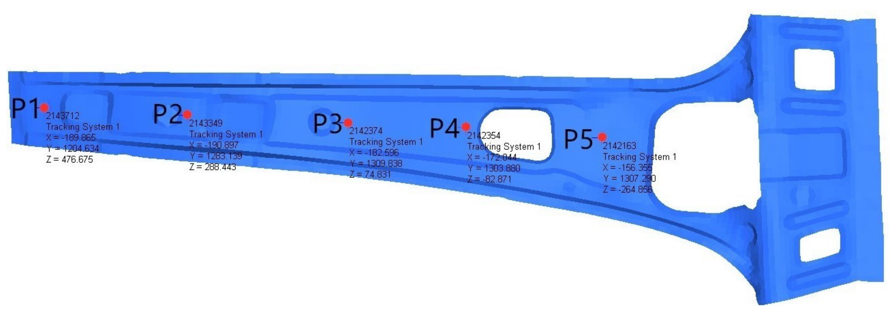
Five locations on the inner surface of the B-pillar inner panel were uniformly selected from top to bottom as measurement points and labeled from P1 to P5. The corresponding node numbers are shown in Figure 6.

Figure 6.
Horizontal layout of the B-pillar inner panel.
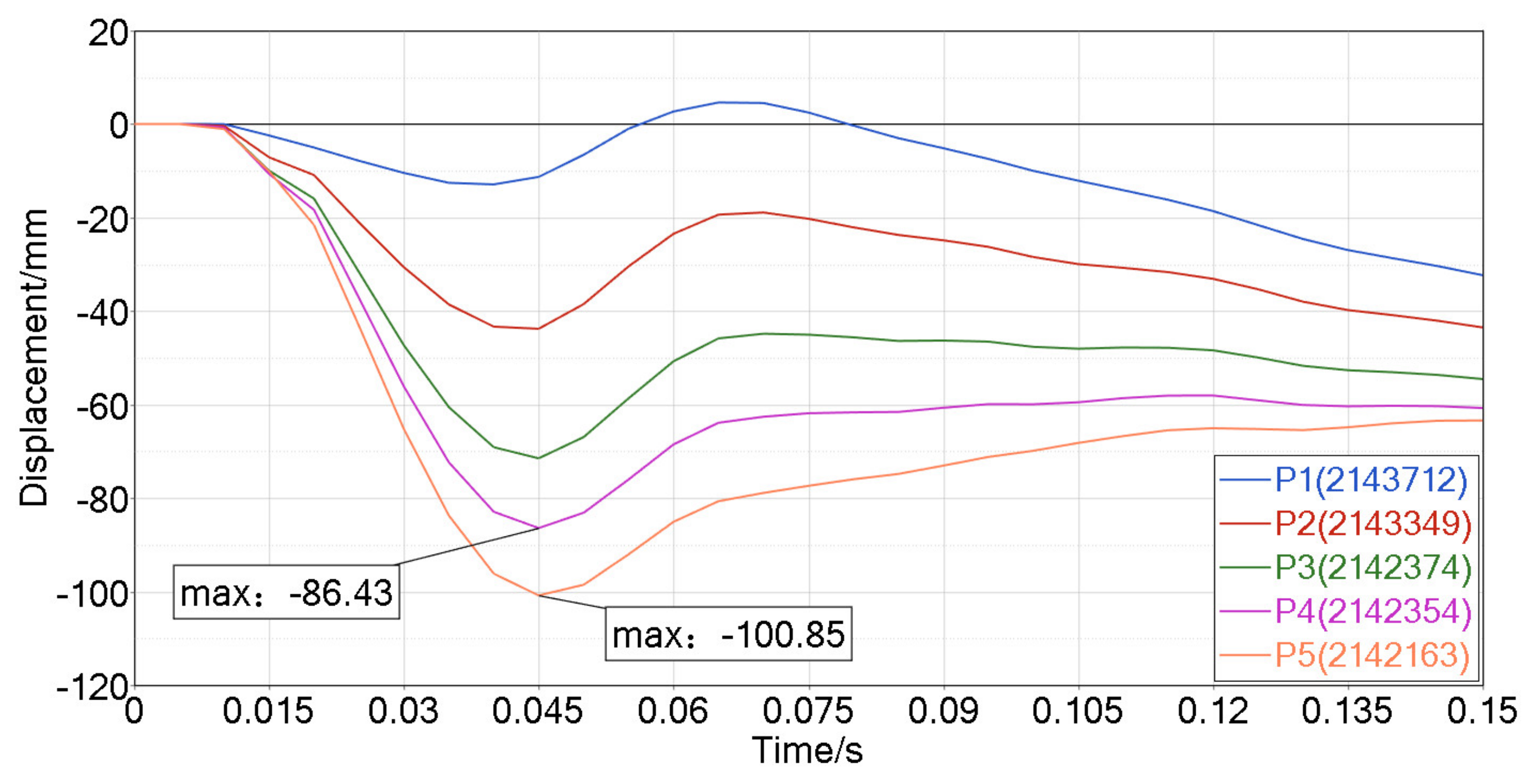
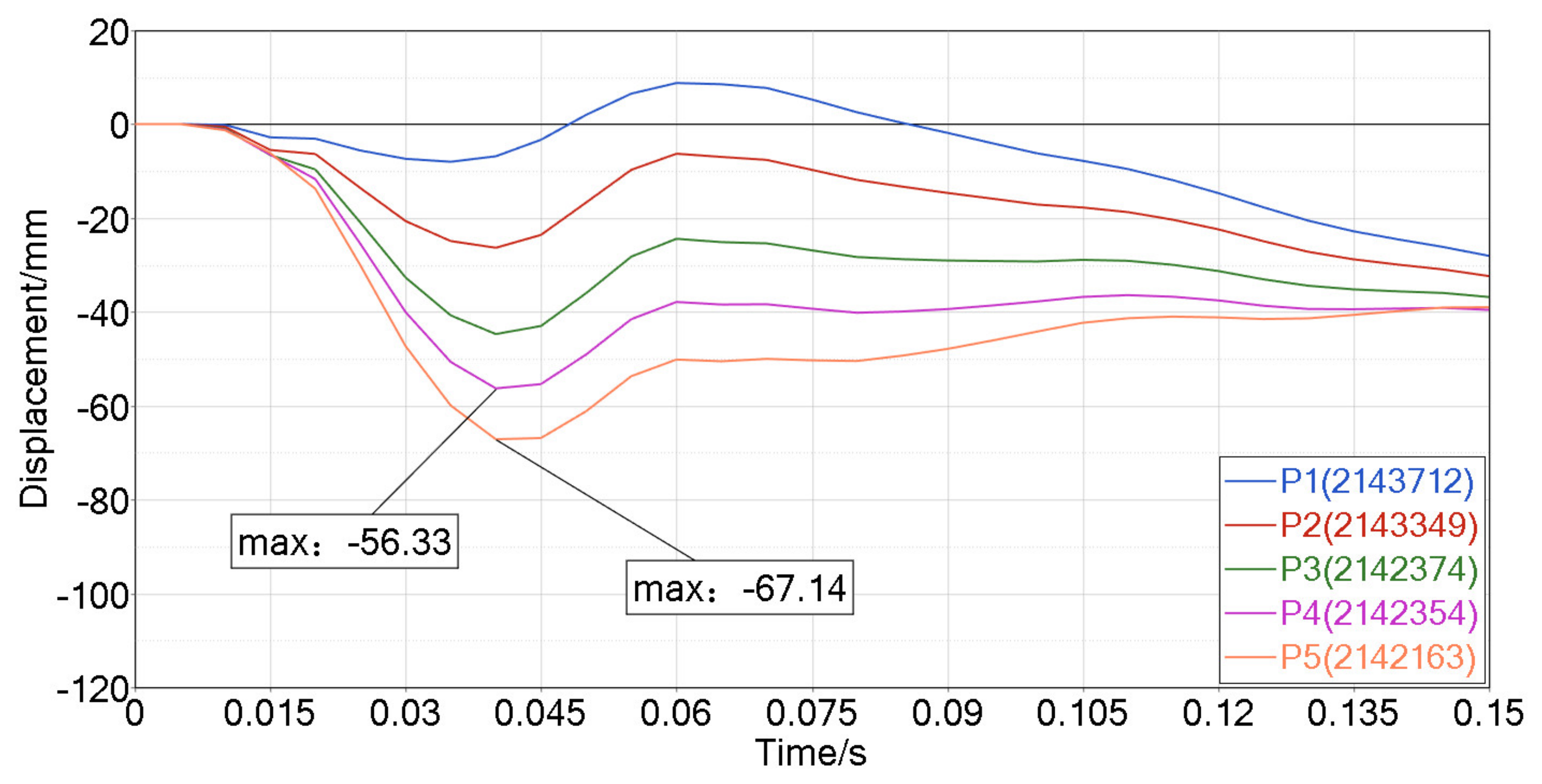
A local coordinate system was then established on the non-deformed right side of the B-pillar inner panel, and the intrusion amount of the side collision was observed at the measuring point. The intrusion amount curve is shown in Figure 7. Points P1 and P2 were above the collision position of the trolley, and the amount of intrusion was small. Given the large deformation at the bottom, point P1 at the topmost position rebounded outside of the initial position within a short period. Points P3 to P5 are in the collision area between the front of the trolley and the vehicle, where the intrusion amount was large and the intrusion trend was consistent. Point P5 had the largest amount of intrusion, followed by P4, and the amount of intrusion at both these points exceeded 80 mm. Many intrusions are observed in the vehicle interior that may harm the human body. The maximum intrusion amount at observation points P4 and P5 was selected as the constraint condition in the vehicle interior noise optimization, and the thickness of the B-pillar inner panel was set as the design variable for subsequent optimization.
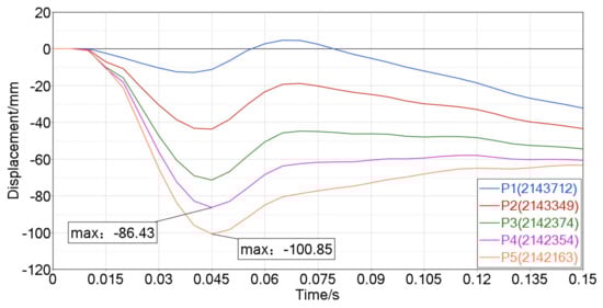
Figure 7.
Amount of intrusion at each point of the B-pillar inner panel.
4. NVH Simulation Analysis
4.1. Working Condition Setting
The X, Y, and Z forces were applied to the left and right engine suspensions of the acoustic-structure coupling model with a magnitude of 1 N. Constraints were set at the spring supports of the front and rear suspensions of the vehicle body to limit the translation and torsion freedom. The analysis frequency was set between 20 Hz and 200 Hz. The position of the main driver’s right ear was selected as the target point in the vehicle, and the A-weighted sound pressure level of the target point was treated as the response [42].
4.2. Vibration and Noise Theory
The noise transfer function (NTF) characterized the correlation between the structure and acoustic characteristics of the internal acoustic cavity. For its low-frequency response, the vehicle body was assumed to be a linear system. Given that the Fourier transform has certain conditional restrictions in its function, to address the vibration problem in a linear system, the ratio of the Laplace transform of the response to the excitation is often used in engineering to obtain the NTF.
The Laplace transform of function is denoted by
where s is a complex variable, t is a time variable, and denote the mass vibration displacement. The differential equation under the action of any exciting force is:
where m is mass, c is the damping coefficient and k is the stiffness coefficient. x, , and denote displacement, velocity and acceleration respectively [43]. The Laplace transform on the above formula is:
where is the Laplace transform of the exciting force function , and denote the initial displacement and initial velocity. By ignoring the homogeneous solution that decays with time, let , and obtain the transfer function of the system as follows:
where and are derived from the Laplace transform of and , both of which denote frequency. The noise transfer function is determined by the system characteristics and reflects the dynamic characteristics of the system.
The sound wave was generated by the propagating vibration of the medium particle, whereas the vibration speed and displacement of the medium particle are physical quantities that describe the sound wave. After treating the main driver’s right ear position as the output node, the acoustic-structure coupling model file was submitted to Optistruct to obtain the A-weighted sound pressure level of the target node in the vehicle.
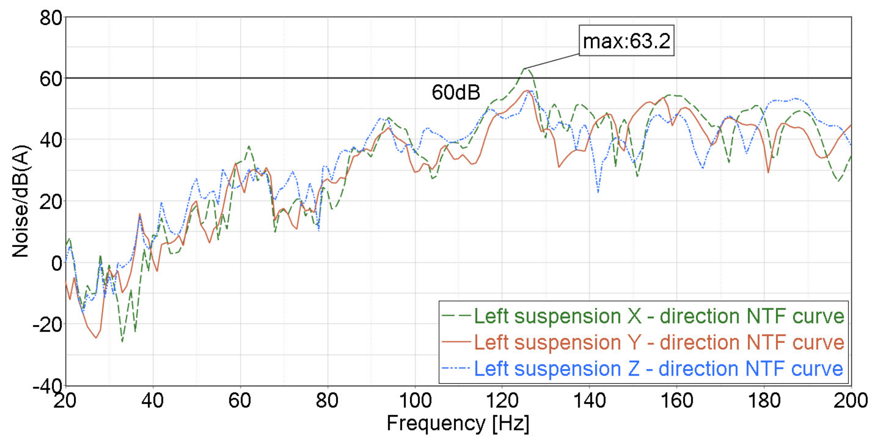
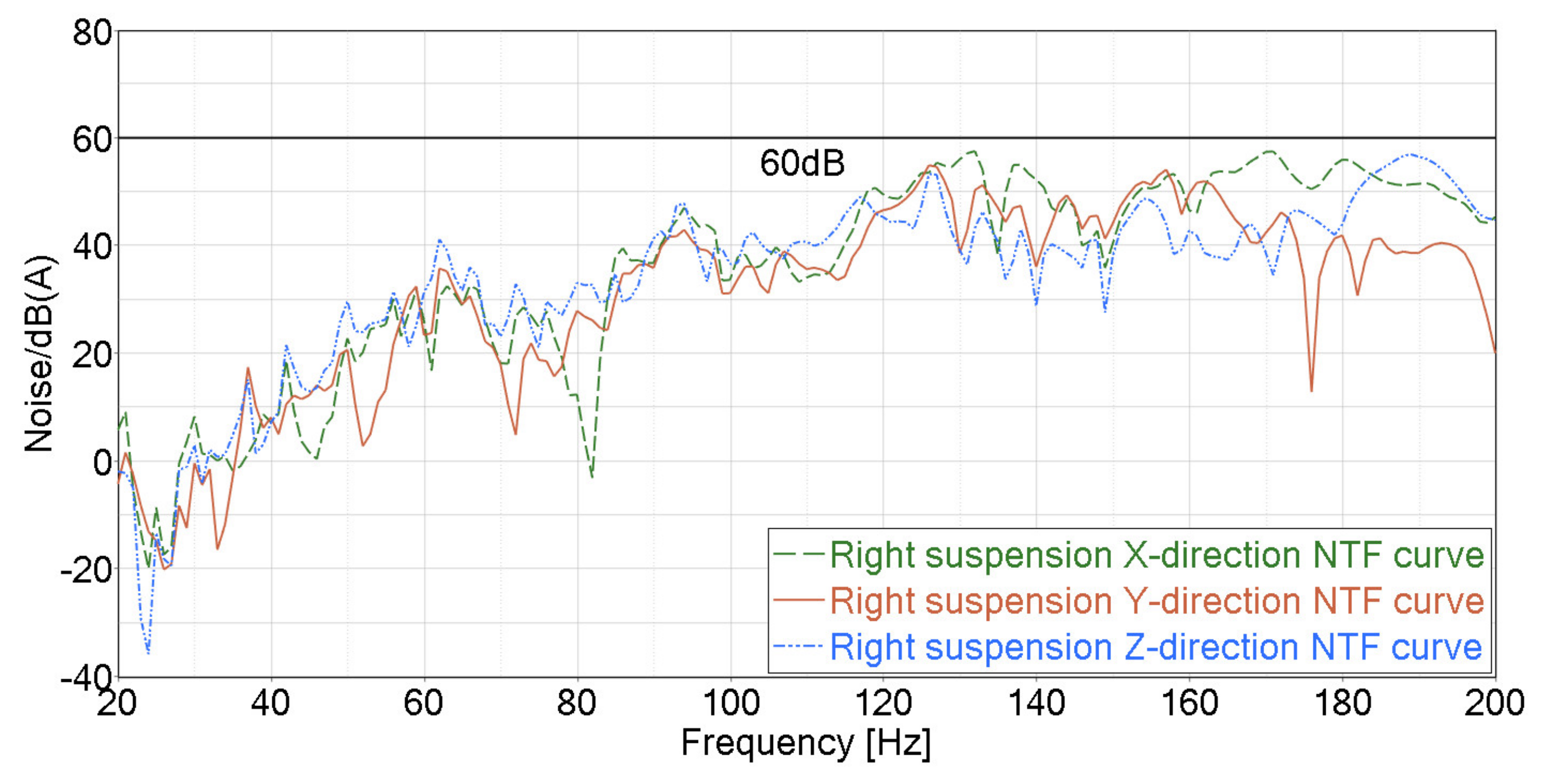
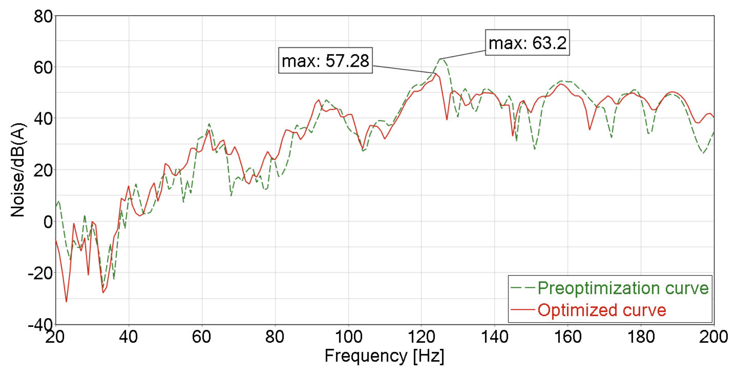
The left and right engine suspension noise transfer function curves are shown in Figure 8 and Figure 9. The logarithm of the ratio between the effective value of sound pressure and the reference sound pressure was multiplied by 20 to obtain the sound pressure level. The reference sound pressure in the air was Pa, which is the lowest sound that the human ear can perceive at 1000 Hz. Given that 0 dB is equivalent to Pa, the sound pressure level in the 0 Hz–40 Hz range corresponding to some frequencies is negative, thereby indicating that the corresponding sound pressure effective value is less than Pa. The sound pressure response of the left engine suspension X path exceeded 60 dB in the 123–127 Hz range, the response reached 63.2 dB at 125 Hz, and the sound pressure response of the five other paths were all below 58 dB. The transfer path of the X direction of the left engine suspension was taken as the research object, and the thickness of the body panel was optimized with the goal of reducing the maximum sound pressure level of the target node and the noise inside the vehicle.
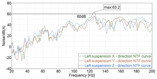
Figure 8.
Left engine suspension noise transfer function curve.
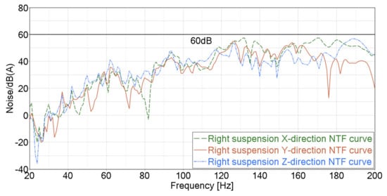
Figure 9.
Right engine suspension noise transfer function curve.
5. Prediction and Optimization of Noise in the Vehicle
5.1. Acoustic Sensitivity Analysis of Panels
In neural network prediction, some unimportant input variables will not only increase the size and complexity of the network but also reduce the prediction accuracy of the model. Therefore, the selection of input variables is a key step in the application of neural network methods. This article performs sensitivity analysis to filter the input variables. Sensitivity indicates the effect of the input variables on the output variables. Given that the body panels contribute differently to the sound pressure level at any position in a vehicle, before training the Elman neural network, a sensitivity analysis of panel thickness should be performed, those panels with a large impact on the output variables should be screened out, and the thickness of these panels should be taken as the input variables of the Elman neural network.
All 36 panels surrounding the sound cavity in the vehicle were labeled, and Hyperstudy was used to analyze the sensitivity of the first-order global modal, the body mass, and the maximum sound pressure level of the target node in a vehicle. Given the large number of variables, the four-resolution partial factor method was selected for the DOE design to avoid confusing the main effect for the second-order cross effect and to take calculation economy into account. Panel sensitivity was outputted using Hypergraph as shown in Figure 10.
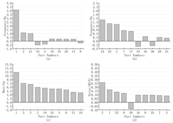
Figure 10.
Panel sensitivity: (a) first order bending modal sensitivity. (b) First order torsional modal sensitivity. (c) Body mass sensitivity. (d) Maximum sound pressure level sensitivity.
As shown in the figure, panels with high response and negative sensitivity are obtained. The B-pillar inner panel is determined via side impact simulation analysis, and the side wall, B-pillar inner panel, C-pillar inner panel, middle bottom panel, rear bottom panel, tail-light inner panel, A-pillar inner panel, and roof are identified as panels that require optimization. The value ranges of the panels are shown in Table 3.
Table 3.
Value ranges of the panels.
5.2. Elman Neural Network
A neural network comprises a large number of interconnected neurons. On the basis of the interconnection among neurons in a network, common network structures mainly include feed forward neural networks, feedback neural networks, and self-organizing neural networks.
The BP neural network is a mature multi-layer feedforward neural network with strong nonlinear mapping characteristics and good generalization ability. When training this network, the forward transmission of information and the back propagation of errors are used to influence the weight in the network. The value and threshold are adjusted to ensure that the predicted output of the BP neural network constantly approaches the expected output.
In the feedback network, the information is transmitted in the forward direction at the same time as the reverse transmission. Feedback of this information can occur between neurons across different network layers or be limited to only a certain layer of neurons. The Elman neural network (ENN) is both a typical feedback network and a dynamic recurrent neural network that is based on the basic structure of the BP neural network with an extra continuation layer added to the hidden layer as a one-step delay operator to achieve the purpose of memory. The system can adapt to time-varying characteristics to enhance the global stability of the network. The Elman neural network has a higher computing power than typical feedforward neural networks and can be used to solve fast optimization problems. The network model established by the Elman neural network can be used in fields with nonlinear time series characteristics given its strong robustness, good generalization ability, strong versatility, and high objectivity.
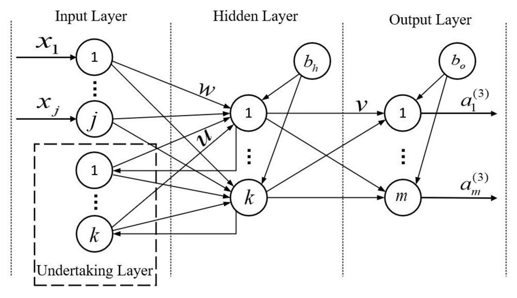
The Elman neural network generally has four layers, namely, the input, hidden, undertaking, and output layers, which are connected similar to a feed forward network. The input layer unit plays a signal transmission role, whereas the output layer unit plays a weighting role. The hidden layer unit has linear and nonlinear activation functions, and the undertaking layer memorizes the output value of the hidden layer unit at the previous moment, which can be regarded as a delay operator with a one-step delay. The output of the hidden layer is self-connected to the input of the hidden layer through the delay and storage of the undertaking layer. However, this self-connection method is sensitive to historical data. The addition of the internal feedback network enhances the ability of the network to process dynamic information. The input, hidden, undertaking, and output layer nodes are denoted by i, h, t, and o, respectively, whereas the number of input, hidden, and output layer nodes are denoted by j, k, and m. The Elman neural network topology is shown in Figure 11.

Figure 11.
Elman neural network topology.
where z and a denote the input and output of each node layer, respectively, whereas and denote the biases of the hidden and output layers. The output of the input layer can be expressed as:
where denote input variable, i = 1, 2, 3,…, j. The hidden layer input (input layer output) can be formulated as:
where h = 1, 2, 3,…, k, is the weight from node i of the input layer to node h of the hidden layer. Equation 6 can take the following matrix form:
The hidden layer output (output layer input) can be formulated as:
where t = 1, 2, 3,…, k, is the weight from node t of the input layer to node h of the hidden layer, and is the output value of the previous generation of hidden layer neuron i. With the continuous increase of input data, the self-loop structure of the undertaking layer transfers the previous state to the current input as the new input data for the current round of training and learning. The hyperbolic tangent function denotes the activation function of the hidden layer neuron [44], which can be formulated as:
The output of the hidden layer is used as the input of the output layer, which can be expressed as:
where o = 1, 2, 3,…, m, is the weight from node h of the hidden layer to node o of the output layer. Equation (10) can be transformed into the following matrix:
The output of the output layer is formulated as:
where is the activation function of neurons in the output layer [44]:
In Equations (5), (6), (8), (10) and (12), the superscripts (1), (2) and (3) denote the input, hidden, and output layers, respectively.
The error function of the output layer neuron is expressed as:
where is the true value of node o in the output layer.
The gradient descent method of the output neuron error is used to correct the weight and threshold of the network, and the change in the weight and threshold of the output layer is formulated as:
The hidden layer weights and thresholds are formulated as:
The undertaking layer weight is expressed as:
5.3. Prediction of Noise Value in the Vehicle
5.3.1. Experimental Design
The thickness of the panels as determined in the side impact and NVH simulation analyses was treated as the input variable, and the maximum sound pressure level of the target point in a vehicle, the body mass, the first-order global modal of the body-in-white, and the maximum intrusion of the B-pillar P4 and P5 points were treated as the output variables. These variables were submitted to Optistruct and LS-DYNA for the simulation calculations, and the generated datasets were used for training and testing the Elman neural network algorithm. To ensure that the input variables took points uniformly in the design interval, the Hammersley method was used for sampling. A total of 200 sets of sample data were obtained and equally divided between the training and test sets.
5.3.2. Algorithm Structure
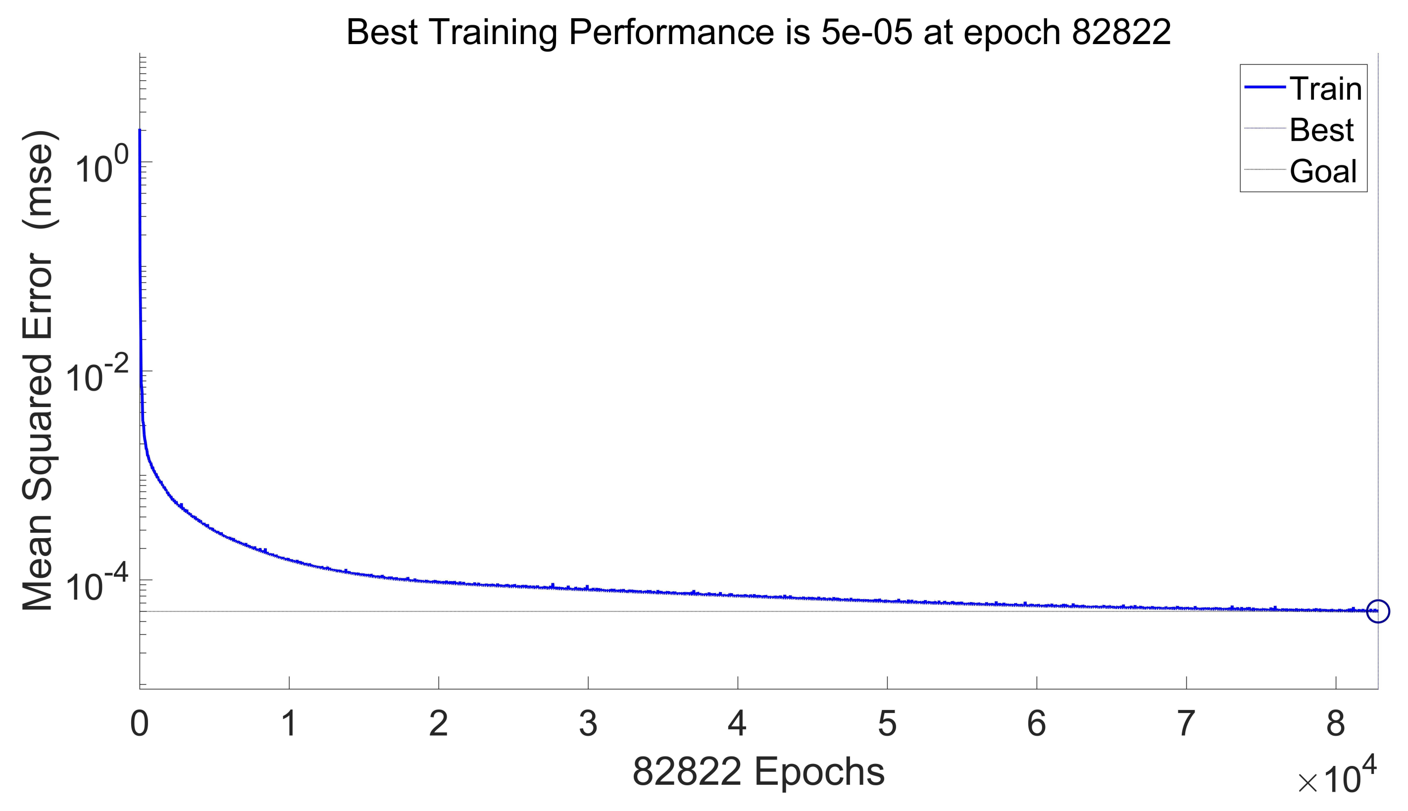
The Elman neural network uses a single hidden layer neural network and has eight and six input and output layer nodes, respectively, as determined by its number of input and output variables. According to Kolmogorov’s theorem, the number of hidden layer nodes was (where j is the number of input layer nodes). This network had a maximum of 200,000 training steps, and the minimum error of the training target was set to .
6. Analysis of Prediction Results
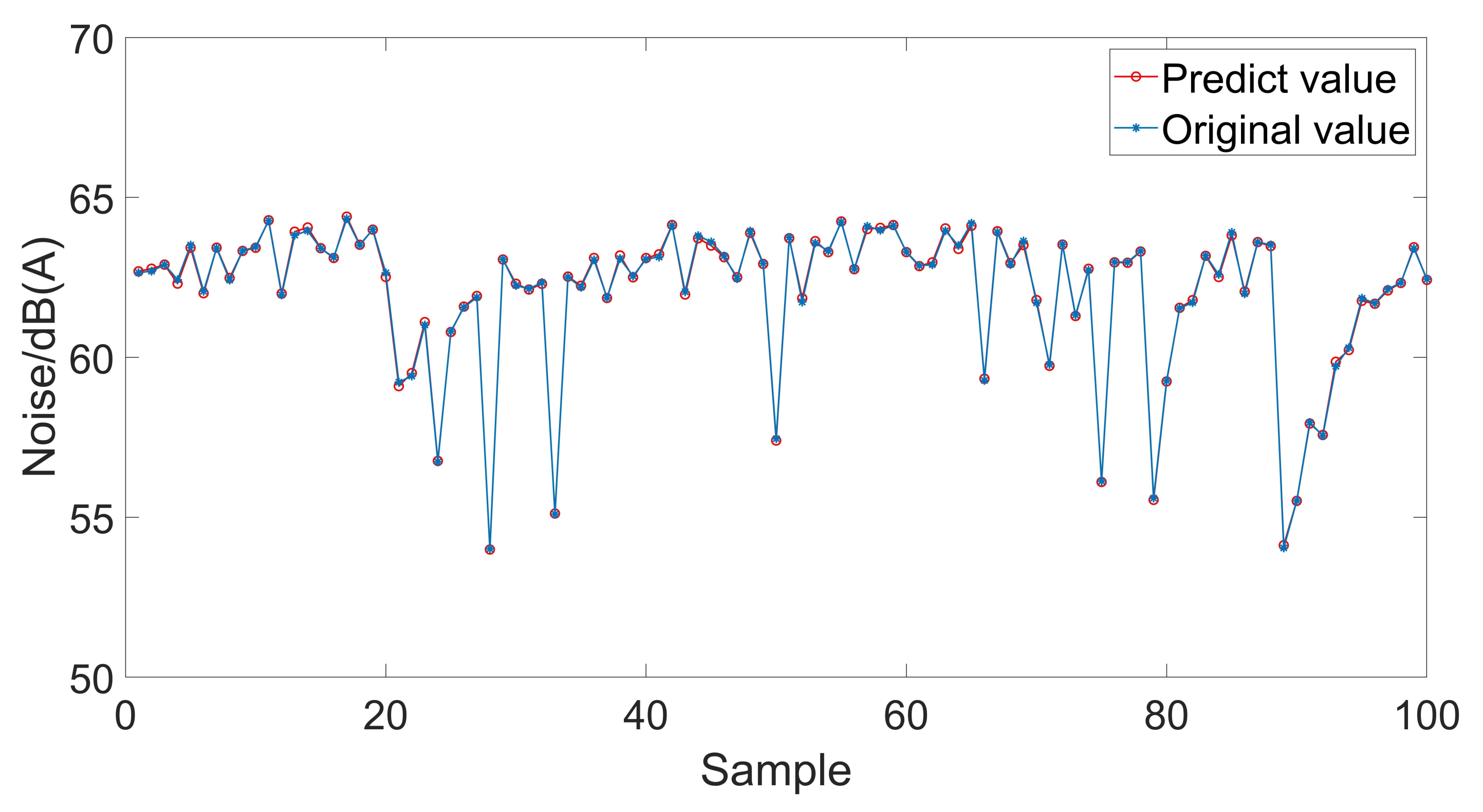
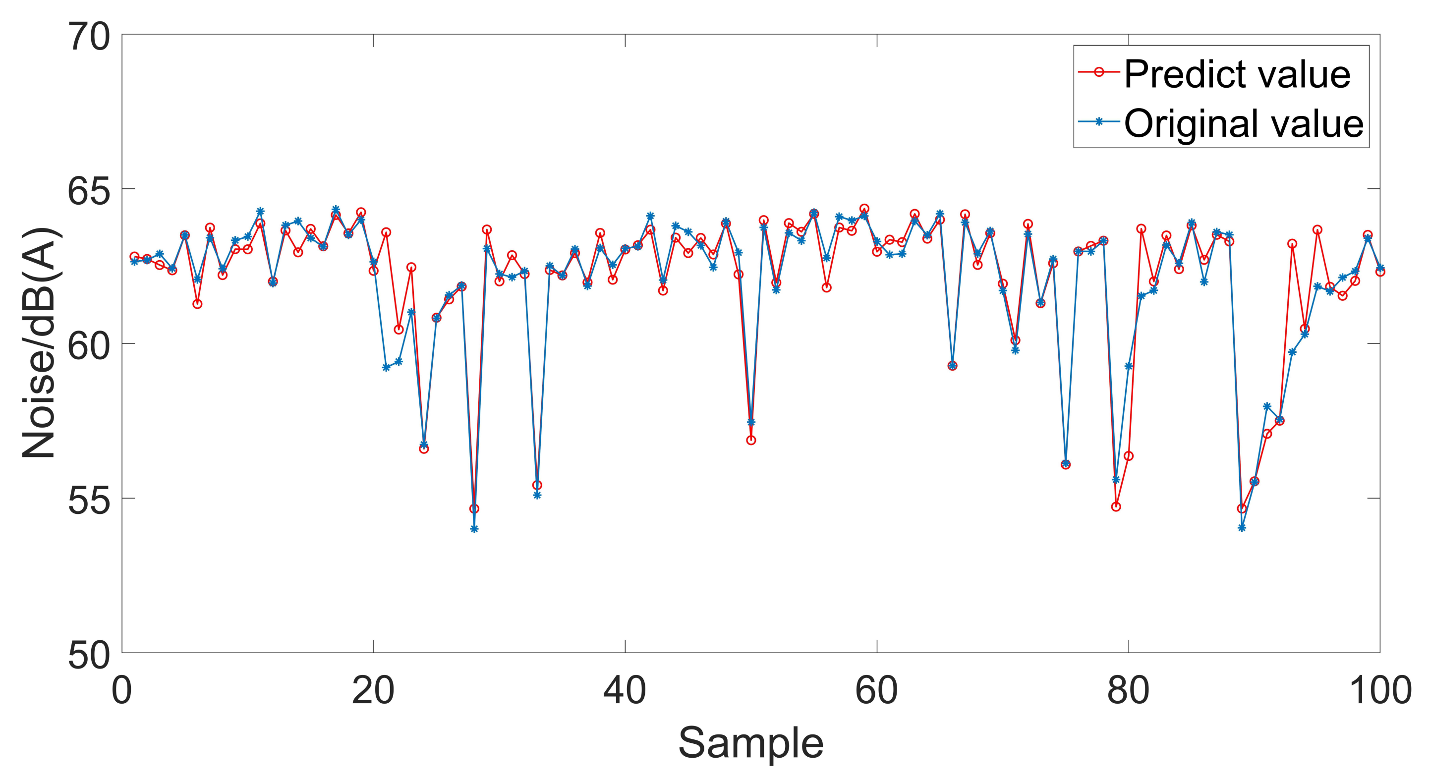
The Elman neural network predicts the maximum sound pressure level of the target point in a vehicle, the body mass, the first-order global modal of the body-in-white, and the maximum intrusion of the B-pillar P4 and P5 points. Figure 12 shows the training process of the Elman neural network, and Figure 13 shows the prediction results for the maximum sound pressure level of the target point in a vehicle. To compare the prediction accuracy of the proposed algorithm with that of other neural network algorithms, the generalized regression neural network (GRNN), BP neural network, and GA-BP neural network were used to predict the maximum sound pressure level of the target point in a vehicle. The prediction results are shown in Figure 14, Figure 15 and Figure 16.
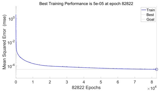
Figure 12.
Elman neural network training process.

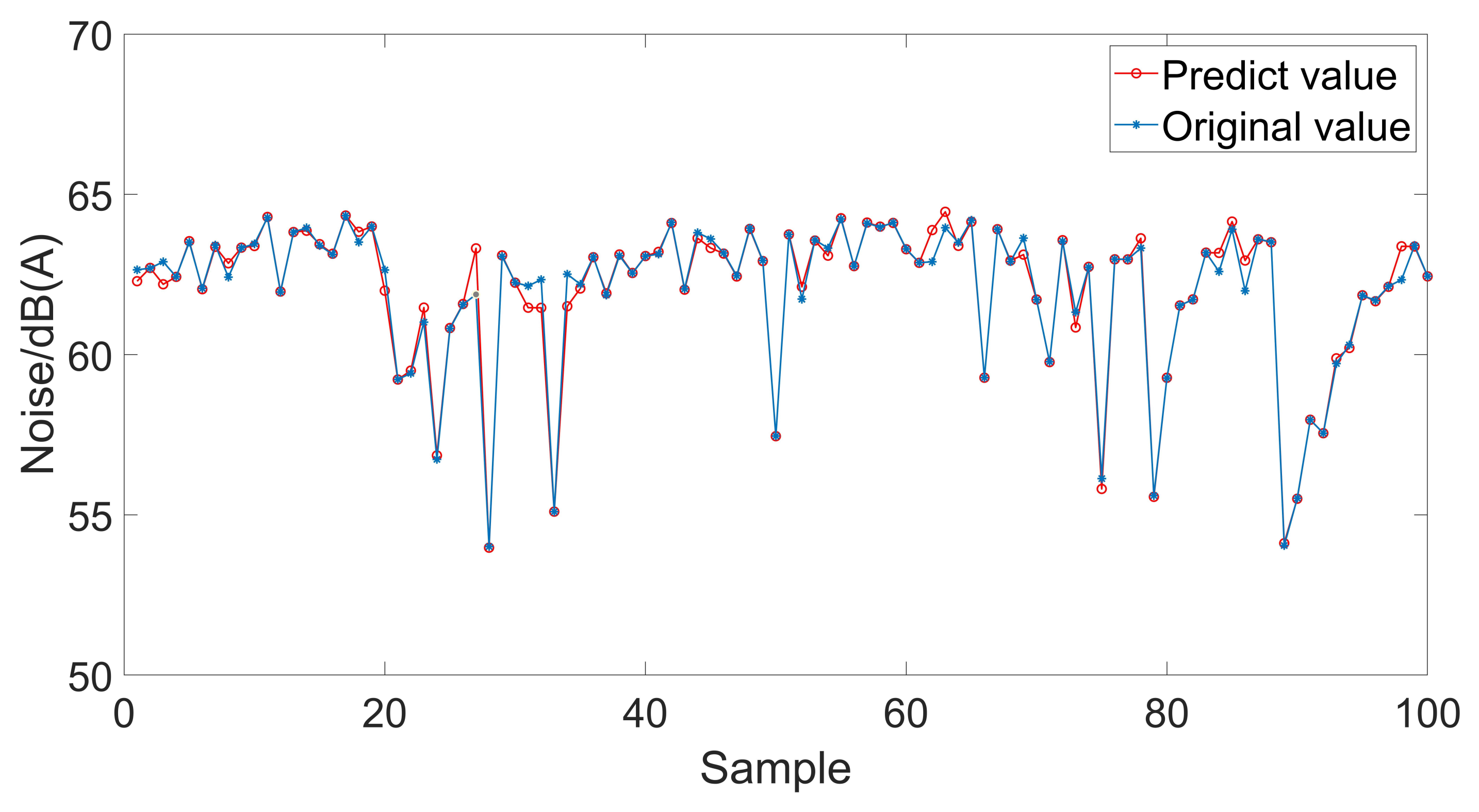
Figure 13.
Elman neural network prediction results.
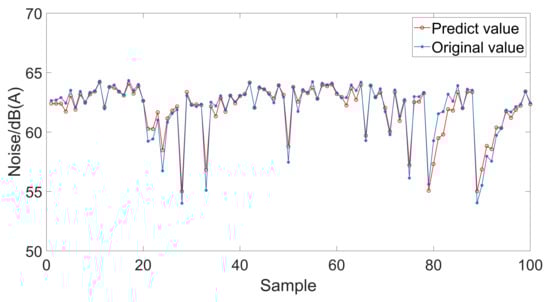
Figure 14.
GRNN neural network prediction results.
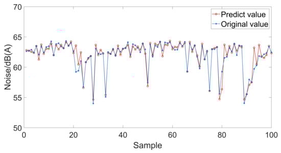
Figure 15.
BP neural network prediction results.
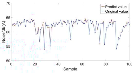
Figure 16.
GA-BP neural network prediction results.
As shown in Figure 12, at the beginning of training, the minimum error decreased sharply, and then the rate of decrease of the minimum error slowed down. At step 82,822, the minimum error reacheed , which met the preset termination conditions. It can be seen from Figure 13, the predicted value of the Elman neural network was highly consistent with the finite element calculation value, and the prediction error was smaller than that of other neural networks. The Elman neural network reported the highest degree of agreement between predicted values and finite element calculations, followed by GA-BP, GRNN, and BP. The mean square error (MSE), root mean square error (RMSE), mean absolute error (MAE), and mean absolute percentage error (MAPE) [45] were used to evaluate the level of prediction error of these models as shown in Table 4.
Table 4.
Comparison of prediction errors of neural network algorithms.
The total number of samples, predicted value, and actual value are denoted by n, , and , respectively. MSE represents the sum of squares of the distance between each predicted value and the actual value. A smaller MSE corresponds to a smaller error and higher prediction accuracy.
RMSE represents the root sign of MSE and is used to measure the deviation between the observed and true values.
Given that dispersion is represented as an absolute value, no positive or negative offset can be obtained. MAE can better reflect the actual situation of the predicted value error.
MAPE represents the ratio of the difference between the predicted and actual values, which can intuitively indicate prediction accuracy.
The prediction errors of the body mass, the first-order global modal of the body-in-white, and the maximum intrusion of the B-pillar P4 and P5 points as predicted by the Elman neural network algorithm are shown in Table 5.
Table 5.
Elman neural network algorithm prediction error.
Table 4 and Table 5 show that the Elman neural network had the smallest prediction error for the maximum sound pressure level of the target point in a vehicle and significantly outperforms the other three neural network algorithms in terms of MSE, RMSE, MAE, and MAPE. The Elman neural network algorithm predicted the mass of the vehicle body, the first-order global modal of the body-in-white, and the maximum intrusion of the B-pillar P4 and P5 points. This algorithm generated small prediction errors that met the prediction accuracy requirements. The enumeration method was applied to enumerate all feasible solutions in the solution set space, and the solution set space was initially discretized. Taking processing accuracy into account, the step length of each input variable in the solution space was set to 0.1, which was equivalent to 1,071,815 feasible solutions. The Elman neural network was then used to predict the maximum sound pressure level at the target point, body mass, first-order modal of the body-in-white, and maximum intrusion of B-pillar P4 and P5 points corresponding to all feasible solutions. By taking the minimum maximum sound pressure level of the target point in a vehicle as the goal, both the body mass and the first-order global modal of the body-in-white did not decrease, whereas the maximum intrusions of the B-pillar P4 and P5 points, as the constraint conditions, were less than 60 mm and 70 mm, respectively. The optimal solution in the feasible solution set was then filtered as:
where is a feasible solution, and , , , , and are the maximum sound pressure levels of the target node, the first-order global modal of the body-in-white, the maximum intrusion amount at point P4, and the maximum intrusion amount at point P5 as obtained by the feasible solution, respectively.
The prediction results were filtered, and the optimal solution conditions that met the constraints were obtained as [1.1,1.2,0.9,1.5,1.5,0.9,2.1,0.9]. To verify the quality of the optimal solution predicted by the Elman neural network algorithm, the thickness of the optimal solution was assigned to the properties of the finite element model, which in turn was submitted to Optistruct and LS-DYNA for the simulation calculation. The noise transfer function curve of the target point in a vehicle and the five-point invasion curve of the B-pillar inner panel are shown in Figure 17 and Figure 18. The maximum sound pressure level of the target point in a vehicle was reduced by 5.92 dB. Compare Figure 18 and Figure 7, the maximum intrusions of points P4 and P5 on the B-pillar inner panel were reduced by 31.1 mm and 33.71 mm, respectively. The comparison between Elman neural network prediction and finite element calculation is shown in Table 6.
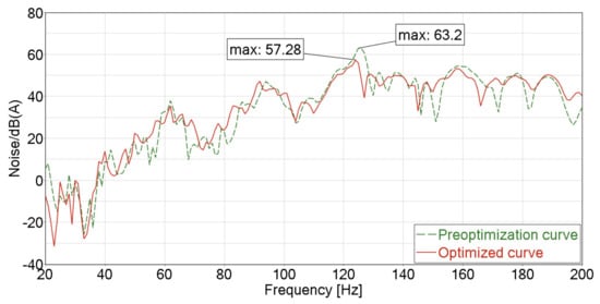
Figure 17.
Left engine suspension X-direction NTF curve.
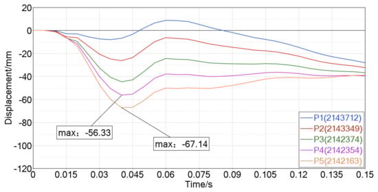
Figure 18.
Amount of intrusion at each point of the B-pillar inner panel.
Table 6.
Comparison between Elman neural network prediction and finite element calculation.
7. Conclusions
Using Hypermesh, the vehicle body acoustic-structure coupling model was established, and a simulation analysis of NVH and side impact was performed. An optimization design method that uses the Elman neural network to comprehensively consider the NVH and side impact performance of a vehicle was then designed. Results show that when the maximum sound pressure level of the target point in the vehicle is reduced, the side impact performance of the vehicle body is significantly improved. The proposed algorithm avoids the shortcomings of single-objective optimization and proves that ride comfort can be enhanced along with the safety of the body design. The prediction errors of the Elman neural network algorithm for each output were within 3%, which meets the prediction accuracy requirements. These findings provide a reference for the application of advanced intelligent algorithms in predicting vehicle interior noise and collision performance and can be used by engineering and technical personnel in actual projects.
Author Contributions
Conceptualization, M.L. (Min Li) and W.Z.; methodology, M.L. (Min Li); software, M.L. (Min Li) and H.Y.; validation, M.L. (Min Li), W.Z., J.L. and X.Z.; formal analysis, W.Z.; writing—original draft preparation, M.L. (Min Li) and M.L. (Mengshan Li); writing—review and editing, M.L. (Min Li) and D.L.; supervision, F.P.; project administration, W.Z.; funding acquisition, J.L. All authors have read and agreed to the published version of the manuscript.
Funding
Financial support was given by NSFC through Grant No. 51575288, as well as the Provincial Natural Science Foundation of Shandong (No. ZR2019MEE072). Both are highly appreciated.
Institutional Review Board Statement
Not applicable.
Informed Consent Statement
Not applicable.
Data Availability Statement
The data presented in this study are available on request from the corresponding author.
Conflicts of Interest
The authors declare no conflict of interest.
References
- Singh, S.; Mohanty, A.R. HVAC noise control using natural materials to improve vehicle interior sound quality. Appl. Acoust. 2018, 140, 100–109. [Google Scholar] [CrossRef]
- Ye, S.G.; Zhang, J.H.; Xu, B. Noise Reduction of an Axial Piston Pump by Valve Plate Optimization. Chin. J. Mech. Eng. 2018, 31, 57. [Google Scholar] [CrossRef] [Green Version]
- Hu, H.X.; Tang, B.; Zhao, Y. Active control of structures and sound radiation modes and its application in vehicles. J. Low Frequency Noise Vib. Act. Control 2016, 35, 291–302. [Google Scholar] [CrossRef] [Green Version]
- Guo, R.; Qiu, S.; Yu, Q.L.; Zhou, H.; Zhang, L.J. Transfer path analysis and control of vehicle structure-borne noise induced by the powertrain. Proc. Inst. Mech. Eng. Part D 2012, 226, 1000–1109. [Google Scholar] [CrossRef]
- Bao, G.Z.; Shao, G.S.; Xia, Z.W.; Den, J.H. Identification and contribution analysis of vehicle interior noise based on acoustic array technology. Adv. Mech. Eng. 2017, 9, 1687814017730031. [Google Scholar] [CrossRef] [Green Version]
- Chen, S.M.; Wang, L.H.; Song, J.Q.; Wang, D.F.; Chen, J. Interior High Frequency Noise Analysis of Heavy Vehicle Cab and Multi-Objective Optimization with Statistical Energy Analysis Method. Fluct. Noise Lett. 2017, 16, 1750017. [Google Scholar] [CrossRef]
- Huang, H.B.; Huang, X.R.; Yang, M.L.; Lim, T.C.; Ding, W.P. Identification of vehicle interior noise sources based on wavelet transform and partial coherence analysis. Mech. Syst. Signal Process. 2018, 109, 247–267. [Google Scholar] [CrossRef]
- Liao, L.Y.; Zuo, Y.Y.; Meng, H.D.; Liao, X.H. Research on the technology of noise reduction in hybrid electric vehicle with composite materials. Adv. Mech. Eng. 2018, 10, 1687814018766916. [Google Scholar] [CrossRef] [Green Version]
- Wu, Y.D.; Li, R.X.; Ding, W.P.; Croes, J.; Yang, M.L. Mechanism Study and Reduction of Minivan Interior Booming Noise during Acceleration. Shock Vib. 2019, 2019, 2190462. [Google Scholar] [CrossRef] [Green Version]
- Lee, H.R.; Kim, H.Y.; Jeon, J.H.; Kang, Y.J. Application of global sensitivity analysis to statistical energy analysis: Vehicle model development and transmission path contribution. Appl. Acoust. 2019, 146, 368–389. [Google Scholar] [CrossRef]
- Huang, H.B.; Wu, J.H.; Huang, X.R.; Ding, W.P.; Yang, M.L. A novel interval analysis method to identify and reduce pure electric vehicle structure-borne noise. J. Sound Vib. 2020, 475, 115258. [Google Scholar] [CrossRef]
- Guo, R.; Zhang, L.J.; Zhao, J.; Zhou, H. Interior structure-borne noise reduction by controlling the automotive body panel vibration. Proc. Inst. Mech. Eng. Part D 2012, 226, 943–956. [Google Scholar] [CrossRef]
- Wang, Y.L.; Qin, X.P.; Lu, L.; Liu, H.M.; Huang, J.J. The noise control of minicar body in white based on acoustic panel participation method. J. Vibroeng. 2016, 18, 1332–1345. [Google Scholar]
- Tian, W.Y.; Yao, L.Y.; Li, L. A Coupled Smoothed Finite Element-Boundary Element Method for Structural-Acoustic Analysis of Shell. Arch. Acoust. 2017, 42, 49–59. [Google Scholar] [CrossRef]
- Wang, Y.L.; Lu, C.H.; Qin, X.P.; Huang, S.; Tan, X.D.; Sun, Y. Control of structure-borne noise for a vehicle body by using power flow analysis and acoustic path participation method. Appl. Acoust. 2020, 157, 106981. [Google Scholar] [CrossRef]
- Wu, X.D.; Kong, Y.; Zuo, S.G.; Liu, P.X. Research on multi-band structural noise reduction of vehicle body based on two-degree-of-freedom locally resonant phononic crystal. Appl. Acoust. 2021, 179, 108073. [Google Scholar] [CrossRef]
- Zhao, W.; Liu, Y.T.; Liu, X.D.; Shan, Y.C.; Hu, X.J. Analysis of Tire Acoustic Cavity Resonance Energy Transmission Characteristics in Wheels Based on Power Flow Method. Appl. Sci. 2021, 11, 3979. [Google Scholar] [CrossRef]
- Hu, X.J.; Liu, X.D.; Shan, Y.C.; He, T. Simulation and Experimental Validation of Sound Field in a Rotating Tire Cavity Arising from Acoustic Cavity Resonance. Appl. Sci. 2021, 11, 1121. [Google Scholar] [CrossRef]
- Kim, Y.D.; Jeong, J.E.; Park, J.S.; Yang, I.H.; Park, T.S.; Muhamad, P.B.; Choi, D.H.; Oh, J.E. Optimization of the lower arm of a vehicle suspension system for road noise reduction by sensitivity analysis. Mech. Mach. Theory 2013, 69, 278–302. [Google Scholar] [CrossRef]
- Zhang, Z.Y.; Zhang, Y.B.; Huang, C.X.; Liu, X. Low-noise structure optimization of a heavy commercial vehicle cab based on approximation model. J. Low Freq. Noise Vib. Act. Control 2018, 37, 987–1002. [Google Scholar] [CrossRef] [Green Version]
- Chen, Y.; Qiu, N.N.; Zang, L.B.; Wei, C.Y.; Li, G.X.; Li, L. Investigation into transmission radiated noise during the acceleration of electric buses based on response surface methodology. Int. J. Vehicle Des. 2020, 82, 205–223. [Google Scholar] [CrossRef]
- Guo, Z.H.; Jie, W.; Lu, H.Y.; Wang, J.-Z. A case study on a hybrid wind speed forecasting method using BP neural network. Knowl.-Based Syst. 2011, 24, 1048–1056. [Google Scholar] [CrossRef]
- Jeong, U.C.; Kim, J.S.; Kim, Y.D.; Oh, J.E. Noise reduction of the automobile multi-mode muffler using differential gap control and neural network control. Proc. Inst. Mech. Eng. Part D 2016, 230, 928–941. [Google Scholar] [CrossRef]
- Ma, C.G.; Chen, C.Y.; Liu, Q.H.; Gao, H.B.; Li, Q.; Gao, H.; Shen, Y. Sound Quality Evaluation of the Interior Noise of Pure Electric Vehicle Based on Neural Network Model. IEEE Trans. Ind. Electron. 2017, 64, 9442–9450. [Google Scholar] [CrossRef]
- Huang, X.R.; Huang, H.B.; Wu, J.H.; Yang, M.L.; Ding, W.P. Sound quality prediction and improving of vehicle interior noise based on deep convolutional neural networks. Expert Syst. Appl. 2020, 160, 113657. [Google Scholar] [CrossRef]
- Wang, Y.S.; Guo, H.; Feng, T.P.; Ju, J.; Wang, X.L. Acoustic behavior prediction for low-frequency sound quality based on finite element method and artificial neural network. Appl. Acoust. 2017, 122, 62–71. [Google Scholar] [CrossRef]
- Zhang, Y.T.; Zhou, J.Y.; Xie, Y.Z. Virtual reality of interior noises of vehicles based on boundary element and neural networks. Neural Comput. Appl. 2018, 29, 1281–1291. [Google Scholar] [CrossRef]
- Peng, J.S.; Xu, L.; Shao, Y.M. Research on the virtual reality of vibration characteristics in vehicle cabin based on neural networks. Neural Comput. Appl. 2018, 29, 1225–1232. [Google Scholar] [CrossRef]
- Qian, K.; Hou, Z.C.; Sun, D.K. Sound Quality Estimation of Electric Vehicles Based on GA-BP Artificial Neural Networks. Appl. Sci. 2020, 10, 5567. [Google Scholar] [CrossRef]
- Liang, Y.; Qiu, L.; Zhu, J.; Pan, J. A digester temperature prediction model based on the elman neural network. Appl. Eng. Agric. 2017, 33, 143–148. [Google Scholar] [CrossRef]
- Li, X.Y.; Wang, Z.P.; Zhang, L. Co-estimation of capacity and state-of-charge for lithium-ion batteries in electric vehicles. Energy 2019, 174, 33–44. [Google Scholar] [CrossRef]
- Abdelhafez, E.; Hamdan, M. Correlation between weather and COVID-19 Pandemic in Jordan. Fresenius Environ. Bull. 2021, 30, 4893–4900. [Google Scholar]
- Li, X.M.; Han, Z.W.; Zhao, T.Y.; Zhang, J.L.; Xue, D. Modeling for indoor temperature prediction based on time-delay and Elman neural network in air conditioning system. J. Build. Eng. 2021, 33, 101854. [Google Scholar] [CrossRef]
- Guo, Z.Q.; Wu, H.X.; Zhao, W.Z.; Wang, C.Y. Coordinated control strategy for vehicle electro-hydraulic compound steering system. Proc. Inst. Mech. Eng. Part D 2021, 235, 732–743. [Google Scholar] [CrossRef]
- Ozturk, I.; Kaya, N.; Ozturk, F. Design of vehicle parts under impact loading using a multi-objective design approach. Mater. Test. 2018, 60, 501–509. [Google Scholar] [CrossRef]
- Lee, Y.; Han, Y.H.; Park, S.O.; Park, G.J. Vehicle crash optimization considering a roof crush test and a side impact test. Proc. Inst. Mech. Eng. Part D 2019, 233, 2455–2466. [Google Scholar] [CrossRef]
- Wu, H.Q.; Kuang, S.J.; Hou, H.B. Research on Application of Electric Vehicle Collision Based on Reliability Optimization Design Method. Int. J. Comput. Methods 2019, 16, 1950034. [Google Scholar] [CrossRef]
- Rashid, A.S.Y.; Ramli, R.; Haris, S.M.; Alias, A. Improving the Dynamic Characteristics of Body-in-White Structure Using Structural Optimization. Sci. World J. 2014, 2014, 190214. [Google Scholar] [CrossRef]
- Qu, X.J.; Liang, H.L.; Zhang, B.C.; Cui, X.Y. Numerical optimization of vehicle noises in multi-peak frequency points based on hybrid genetic algorithm and simulated annealing. J. Vibroeng. 2016, 18, 2613–2625. [Google Scholar] [CrossRef]
- Liu, Z.; Yuan, S.A.; Xiao, S.H.; Du, S.Z.; Zhang, Y.; Lu, C.H. Full Vehicle Vibration and Noise Analysis Based on Substructure Power Flow. Shock Vib. 2017, 2017, 8725346. [Google Scholar] [CrossRef] [Green Version]
- Chen, H.; Lu, C.H.; Liu, Z.E.; Shen, C.R.; Sun, Y.; Sun, M.L. Structural Modal Analysis and Optimization of SUV Door Based on Response Surface Method. Shock Vib. 2020, 2020, 9362434. [Google Scholar] [CrossRef]
- Wang, Y.S.; Shen, G.Q.; Guo, H.; Tang, X.L.; Hamade, T. Roughness modelling based on human auditory perception for sound quality evaluation of vehicle interior noise. J. Sound Vib. 2013, 332, 3893–3904. [Google Scholar] [CrossRef]
- Jin, X.X.; Zhang, L.J.; Jiang, H. Automobile Vibration Analysis; Tongji University Press: Shanghai, China, 2002; pp. 46–56. [Google Scholar]
- Yu, S.W. Case Analysis and Application of MATLAB Optimization Algorithm; Tsinghua University Press: Beijing, China, 2015; pp. 64–68. [Google Scholar]
- Kayaalp, K.; Metlek, S.; Ekici, S.; Sohret, Y. Developing a model for prediction of the combustion performance and emissions of a turboprop engine using the long short-term memory method. Fuel 2021, 302, 121202. [Google Scholar] [CrossRef]


Publisher’s Note: MDPI stays neutral with regard to jurisdictional claims in published maps and institutional affiliations. |
© 2021 by the authors. Licensee MDPI, Basel, Switzerland. This article is an open access article distributed under the terms and conditions of the Creative Commons Attribution (CC BY) license (https://creativecommons.org/licenses/by/4.0/).