Use of Seismic Spectral Decomposition, Phase, and Relative Geologic Age as Attributes to Improve Quantitative Porosity Prediction in the Daqing Field, China

Abstract

The high production potential of the Daqing oilfield in China is recognized for seismically thin sand bodies that usually are not resolved with conventional seismic data. The present study assesses the usefulness of applying seismic multi-attribute analysis to bandwidth extended data in resolving and making inferences about these thin layers. In thin layers, tuning can obscure relationships between seismic amplitude and rock properties. In such cases, the seismic phase varies with the layer impedance and may hence aid in reservoir characterization. A seismically derived relative geologic age may also be a useful attribute in predicting rock properties because it helps define the stratigraphic position of a layer. When utilized in multi-attribute analysis in the Daqing field, spectral decomposition amplitude, phase, and a relative geological age attribute to improved prediction of well log effective porosity from seismic data and are preferentially selected by stepwise regression. The study follows standard methodology by implementing seismic multi-attribute analysis and discusses the improvement of applying it to bandwidth extended data. This will include a combination of attributes such as relative geologic age, phase, amplitude, and the magnitude components of spectrally decomposed data.

1. Introduction

The characterization of layers below seismic resolution is a fundamental problem in reservoir modeling especially when there are variations in the reservoir properties away from well control. Multi-attribute seismic analysis [1] is a commonly used technique to extrapolate petrophysical properties from logs to 3D-seismic volumes using seismic attribute traces at well locations as training data. The main goal is to find operators to extrapolate rock properties from log data using seismic data, particularly seismic attributes, which can be defined as any mathematical transformation of the seismic trace [2]. For example, Ray et al. [3] applied the multi-attribute technique to generate an effective porosity volume and successfully characterized a geologically complex reservoir. Abdulaziz [4] applied multi-attribute analysis to porosity prediction in a variety of formations, finding that optimal attributes vary a great deal with geology and seismic data quality.

These studies extracted seismic attributes from a conventional post-stack seismic volume as input, and in some cases, using basic attributes such as frequency filters and amplitude-related attributes to correlate to rock properties. Mora et al. [2] applied multi-attribute analysis with attributes extracted from a spectrally broadened volume and compared the results with those obtained by application of multi-attribute analysis to conventional seismic data in the Daqing field; they achieved statistically significant improved prediction accuracy and precision when using the spectrally broadened volume as input data. In that paper and this study, the spectrally broadened volume is obtained by sparse-layer inversion using basis pursuit decomposition [5]. The bandwidth extension algorithm is fully described and tested in [5] and theoretical aspects of the validity of the bandwidth extension are discussed and demonstrated in [6].

In this paper, our objective is to improve the accuracy and resolution of porosity prediction in the Daqing field, China, utilizing the spectral decomposition of bandwidth extended seismic data. The use of the seismic phase in rock properties prediction is investigated and the study introduces a novel seismic attribute termed relative geologic age. A comparison between predictions with spectral decomposition amplitude, magnitude, phase, and relative geologic age, in addition to the results obtained with conventional attributes—such as those utilized by [1] in the multi-attribute analysis—will be discussed.

The Daqing field and, more specifically, the Qingshankou-Putahoa/Shaertu petroleum system have been broadly explored [7]. Hydrocarbons have been produced from thick reservoirs and potential has been identified on thinner layers [7] but it has been difficult to detect and correlate reservoirs that are significantly thinner than conventional seismic resolution, which is approximately ¼ wavelength at the dominant frequency of the original seismic data (about 33 m for this dataset in the Daqing field). In the study area, well logs reveal hydrocarbon-bearing intervals with thicknesses ranging from 1 to 15 m that cannot be seismically resolved.

The spectrally broadened seismic data has been previously shown to yield more accurate porosity predictions in this field (Mora et al., 2020). Considering the reservoirs are greatly below the limit of seismic resolution for the original seismic data, bandwidth extended data are used as inputs to extract seismic attributes and evaluate the prediction improvement when using seismic attributes that are not usually employed for such purposes [1]. The present study specifically utilizes spectral decomposition amplitude, magnitude, and phase attributes and employs a relative geologic age volume derived from picked horizons. Then, constrained least squares spectral analysis [8] is implemented to perform spectral decomposition. The inputs to the multi-attribute analysis are the amplitude, magnitude, and phase attributes extracted at each frequency. The attributes are divided into four groups: conventional attributes (Group 1), conventional and relative geologic age (Group 2), conventional and spectral decomposition attributes (Group 3), and all the above (Group 4). The multi-attribute analysis is performed separately for each group and the generated porosity volumes are compared. The resulting accuracy, precision, statistical significance, and resolution in the determination of layer porosity are quantified and contrasted.

2. Dataset

The dataset consists of a subset of a 3D seismic survey (for details see [2]), covering an area of about 4 km² (Figure 1a), consisting of spectrally broadened data (Figure 1b) and 24 wells all including density-derived porosity logs.

2.1. Sparse-Layer Inversion

Zhang and Castagna [5] presented an inversion approach using the fact that any local earth-impedance structure can be represented by the superposition of a limited number of layers; thus, the seismogram can also be represented as the superposition of a limited number of layer responses. This inversion assumes a sparse number of layers and can be parameterized to resolve thinner intervals than can generally be obtained with sparse-spike inversion methods [5].

The sparse-layer inversion is accomplished using basis pursuit [9] by minimizing the objective function:

$$\min \left[\parallel \mathit{d}-\mathit{G}\mathit{m}{\parallel }_2^{ }+\lambda \parallel \mathit{m}{\parallel }_1\right],$$

(1)

where m are the model parameters (analogous to a reflectivity series) that indicate the magnitudes of impulse pairs that sum to form the reflectivity series; $\mathit{d}$ is the seismic trace; and $\mathit{G}$ corresponds to a dictionary of pre-defined seismic layer responses. This objective function minimizes the mean-squared error of the fit to the data and introduces sparsity by minimizing the L1 norm of the solution [9]. The seismic responses are obtained by convolving the seismic wavelet with reflectivity patterns that are designed using even and odd impulse pairs with a range of allowable thicknesses defined by geological a priori information. This removes the bias of the sparsity constraint against seismically thin layers [6]. λ is the regularization parameter that acts to balance the inverted reflectivity resolution and noise. Increasing this parameter decreases the resolution of the inverted reflectivity and decreasing it too much could cause noise amplification. The optimum value of λ is determined empirically and depends on the data and earth structure.

Well logs are not used as an initial model for sparse-layer inversion, which operates on a trace-by-trace basis. The output of this technique is an inverted reflectivity series that is filtered to a frequency band which subjectively best balances the resolution, stability, and accuracy of the synthetic ties to wells. The output filtered volume is referred to as spectrally broadened seismic data [2].

Lian and Castagna [6] shows that spectral broadening accomplished by using sparse-layer inversion can be valid if the data quality permits, and the subsurface can be represented as a sparse number of layers. The study concluded that in a worst-case scenario with a highly stratified random earth reflectivity, no practical spectral broadening could be achieved outside the band of the original data. However, the researchers reasoned that this extrapolation could be useful in boosting the high-frequency signal within the original seismic bandwidth more than the high-frequency noise in spectral bluing, hence improving the seismic resolution within the original band of the data.

2.2. Seismic Attributes

Seismic attributes can refer to any quantitative measurement derived from seismic data. Taner et al. [10] divided attributes into geometrical and physical categories. The first group is generally used to enhance the visibility of geometrical characteristics of seismic data, such as dip, azimuth, and continuity. The second group refers to the physical parameters of the subsurface and hence is related to impedance. The main subgroups for this type of attribute are amplitude, phase, and frequency. Barnes [11] recognized amplitude and phase as fundamental attributes from which other attributes are derived. He classified attributes by dimensionality, in depth or time, and as instantaneous or local [12].

Barnes [13] stated that complex seismic trace analysis treats the seismic trace as a continuous set of sinusoidal segments whose properties are recorded by the trace’s instantaneous amplitude, phase, frequency, and relative amplitude change. Instantaneous amplitude is a measure of reflection strength and is commonly used. However, its interpretation is not straightforward when dealing with thin beds. The instantaneous phase and cosine of the phase permit reflection continuity to be better described. While the instantaneous phase shows sharper vertical breaks due to phase wraparound, the cosine of the phase is a continuous waveform analogous to perfect automatic gain control (AGC). It removes all amplitude information that may increase apparent reflection continuity.

Stark [14] introduced the relative geologic age volume. To generate such volume, each seismic sample is assigned an estimated geologic age by imputing previously interpreted reflectors and interpolating between them. This methodology assumes that relative geologic time values increase with depth. The volume has the same dimensions and coordinates as the input seismic data, with each color representing a constant age. The age estimation here is relative, as we can determine which horizon is older or younger in a group but not what is the actual geologic age value of it. Stark [14] presented a detailed explanation of the workflow that generated the relative geologic age volume, including some applications of it. The present study considers relative geologic age volume as simply another seismic attribute to be included in the multi-attribute process.

3. Method and Results

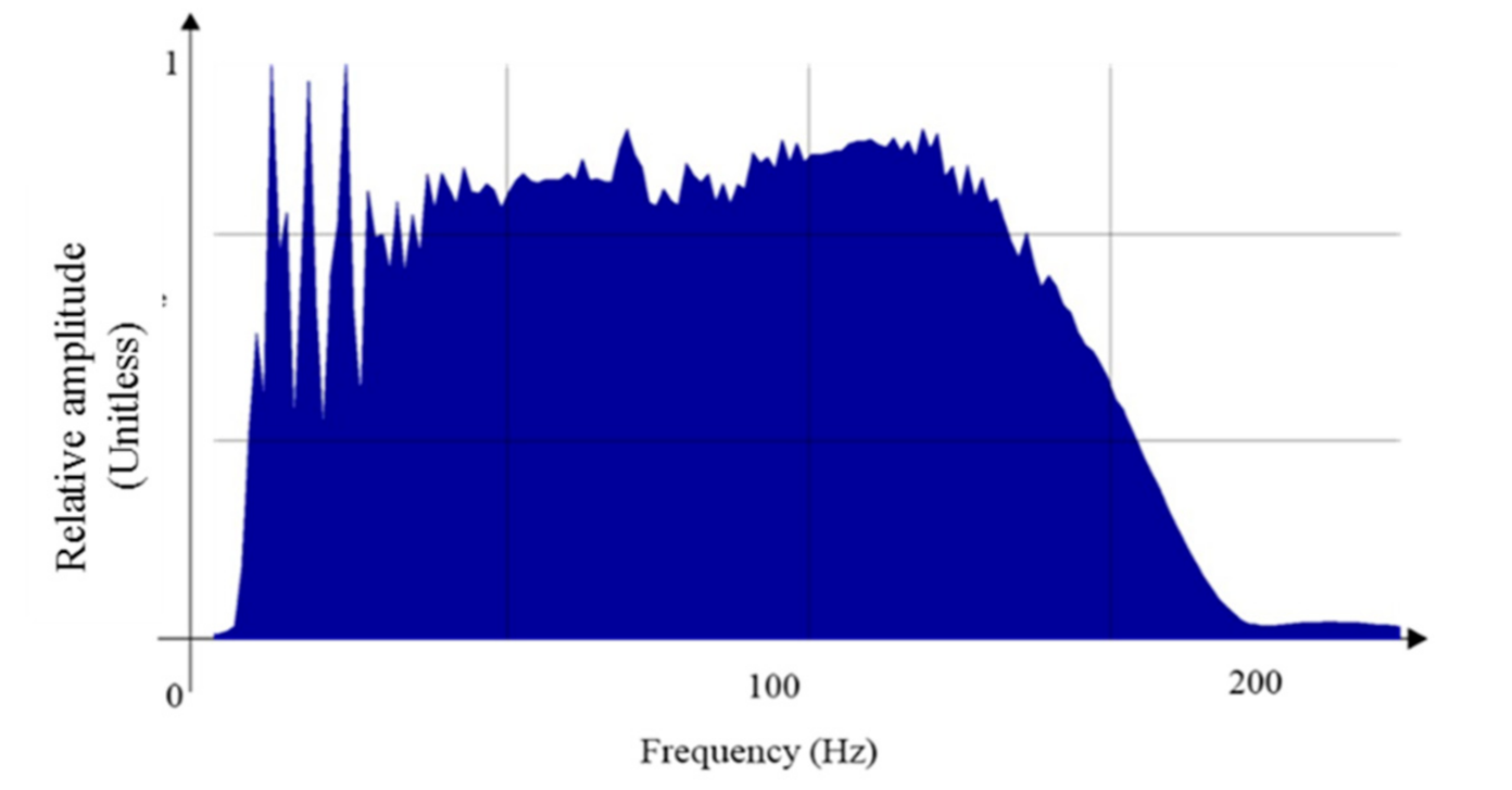
The approach here is to apply the multi-attribute analysis [1] to predict a relationship between porosity and seismic data. Based on the relationship, a porosity volume is generated with training data (21 porosity logs), filtered to a maximum cutoff frequency of 100 Hz, and a series of seismic attributes obtained by applying transforms to a spectrally broadened seismic volume. The logs are filtered to 100 Hz because this is sufficient to show the most significant reservoir layers in the Daqing field. Applying higher frequencies from the logs than necessary will require a porosity prediction algorithm, resulting in degraded predictive accuracy and stability. Then, stepwise regression [15] is applied to selected groups of attributes separately to determine the attributes from each group used to predict porosity. The attributes are added one at a time in the order of the stepwise regression until the validation error starts increasing. This methodology is implemented to determine the number of attributes that will be used to perform the rock property prediction throughout the seismic volume [2]. It will not necessarily select the best possible attribute combination but rather a useful one. In addition, this procedure is further validated with three out-of-sample blind wells that are not utilized in the training. Porosity is predicted for each group and the results are compared to determine the accuracy, resolution, and statistical significance of the predictions. In this study, the spectrally broadened seismic volume is considered a seismic attribute, without any requirement or conclusion regarding the accuracy or completeness of the inferred high-frequency content (Figure 2). The spectrally broadened data has a high-frequency cutoff of about 150 Hz that is more than twice the original seismic bandwidth. The comparison of the original and spectrally broadened data is presented in [2]. The rock properties prediction is an empirical statistical approach that can leverage geological correlations that are not comprehended by a rock properties inversion based entirely on inverting the physics of wave propagation. For this reason, it is not required that the spectral broadening be physically correct such that it will reproduce the seismic data acquired at those frequencies. However, it is required that the spectral broadening be useful for the research purpose, determined by the well-to-seismic tie and the validation results of the blind out-of-sample tests [2].

Figure 2 presents the amplitude spectrum of spectrally broadened data.

3.1. Well-Tie

Using a statistical wavelet derived from the seismic data spectrum, the correlation coefficient of synthetic to spectrally broadened seismic data varied between 0.70 and 0.85 in the 20 wells. No stretch or squeeze was applied in any case.

Figure 3 shows an example of a synthetic tie for one well and the wavelet used.

3.2. Attribute Generation and Classification

Seismic attributes were calculated from spectrally broadened data and classified into four groups, in which Group 1 is a set of conventional and well-known attributes, as listed below [1]:

• amplitude envelope;
• amplitude weighted cosine phase;
• amplitude weighted frequency;
• amplitude weighted phase;
• apparent polarity;
• average frequency;
• cosine of the instantaneous phase;
• derivative;
• derivative instantaneous amplitude;
• dominant frequency;
• energy;
• filter 05/10 15/20;
• filter 15/20 25/30;
• filter 25/30 35/40;
• filter 35/40 45/50;
• filter 45/50 55/60;
• instantaneous frequency;
• instantaneous phase;
• integrate;
• integrate absolute amplitude;
• x-coordinate;
• y-coordinate;
• quadrature trace;
• second derivative;
• second derivative instantaneous amplitude; and
• semblance.

Time Group 2 includes all attributes from Group 1 in addition to a relative geologic age attribute (inline shown in Figure 4), which was obtained by building a volume of several interpreted seismic horizons and interpolating the fractional position between horizons.

Figure 4 shows an inline of the relative geologic age volume.

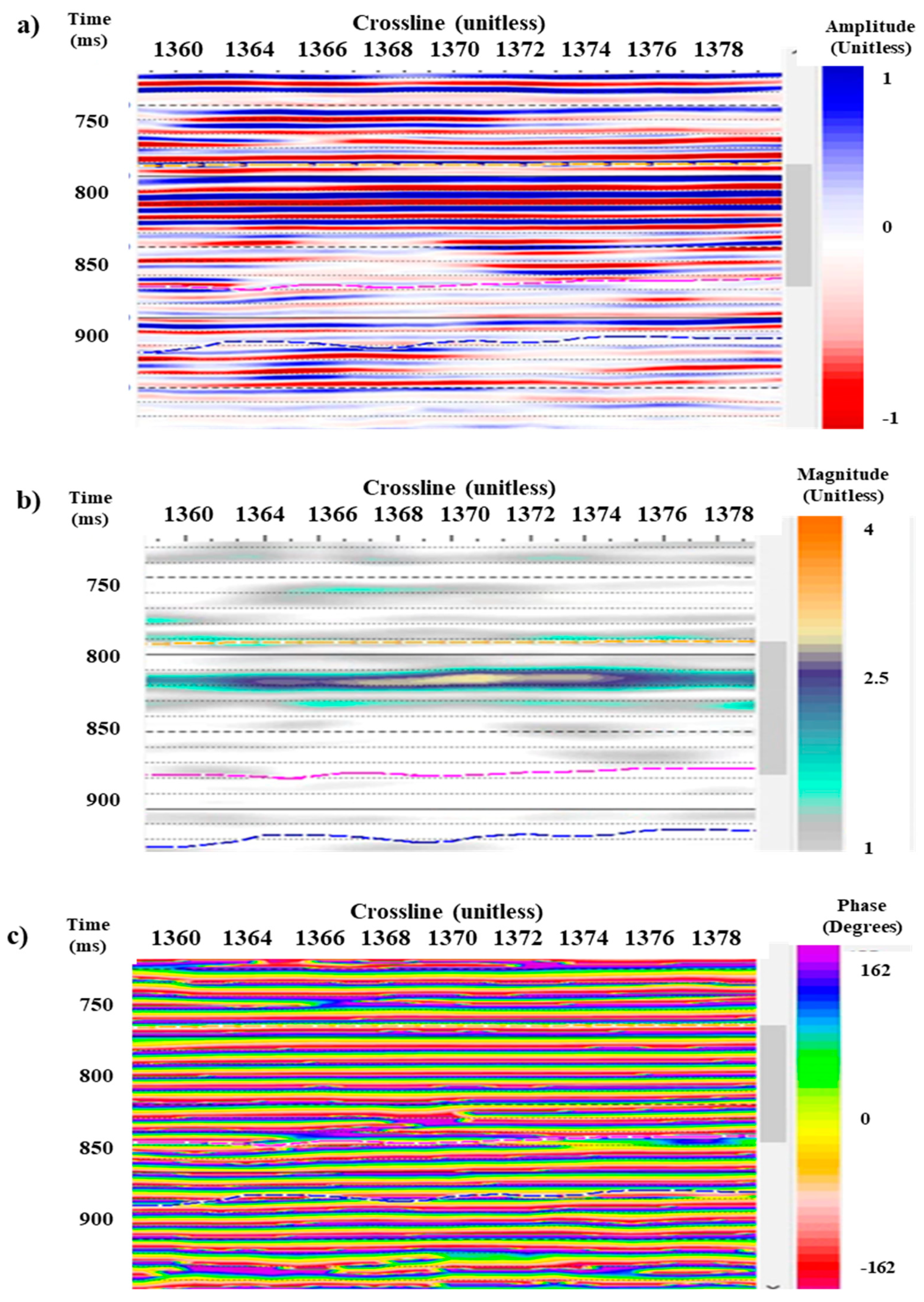
Constrained least squares spectral analysis (CLSSA) as presented in [8] is a spectral decomposition technique that achieves better time–frequency resolution than the commonly used the Fourier transform and continuous wavelet transform (CWT) methods. In this study, CLSSA was implemented to extract the amplitude, phase, and magnitude components from spectrally broadened seismic data every 10 Hz from 10 to 130 Hz. Group 3 includes all attributes from Group 1 in addition to volumes of amplitude, magnitude, and phase components at each selected frequency from the CLSSA spectral decomposition. The cosine of the phase component at each frequency was also included.

Figure 5 shows a section of amplitude, magnitude, and phase for the isofrequency volume at 100 Hz.

Group 4 includes all attributes in Groups 1 to 3.

3.3. Attribute Selection

Stepwise regression was done separately for each group to select the best attributes to predict porosity.

Table 1. Top ten attributes selected by stepwise regression to predict porosity.

Group 1	Group 2
Cosine Instantaneous Phase	Cosine Instantaneous Phase
Integrated Absolute Amplitude	Relative Geologic Age
Filter 5 Hz/10 Hz–15 Hz/20Hz	Filter 5 Hz/10 Hz–15 Hz/20Hz
X-Coordinate	Filter 45 Hz/50 Hz–55 Hz/60Hz
Filter 45 Hz/50 Hz–55 Hz/60Hz	Average Frequency
Average Frequency	X-Coordinate
Amplitude Weighted Phase	Filter 55 Hz/60 Hz–65 Hz/70Hz
Amplitude Weighted Cosine Phase	Y-Coordinate
Quadrature Trace	Instantaneous Frequency
Raw Seismic	Filter 35 Hz/40 Hz–45 Hz/50Hz
Group 3	Group 4
Cosine Instantaneous Phase	Cosine Instantaneous Phase
Magnitude at 50 Hz	Relative Geologic Age
Phase at 30 Hz	Cosine of the Phase at 110 Hz
Cosine of the Phase at 110 Hz	Phase at 30 Hz
Magnitude at 30 Hz	Filter 45 Hz/50 Hz–55 Hz/60Hz
Amplitude at 70 Hz	Semblance
Filter 45 Hz/50 Hz–55 Hz/60Hz	Average Frequency
Cosine of the Phase at 70 Hz	Cosine of the Phase at 70 Hz
Cosine of the Phase at 30 Hz	Phase at 70 Hz
Magnitude at 50 Hz	Cosine of the Phase at 30 Hz

shows the top ten selected attributes in each group.

Cosine of the instantaneous phase was selected by stepwise regression as the best attribute in all cases, followed by relative geologic age when available. For Groups 3 and 4, phase attributes represented 50% and 60% of the top ten, respectively. The elimination of the need for x and y coordinates for both Groups 3 and 4 suggests that the inclusion of spectral decomposition volumes compensates for any lateral drift in the prediction calibration and may account for the greater lateral variability in the predicted porosity resulting from these groups (see below).

3.4. Porosity Versus Cosine of the Phase Modeling

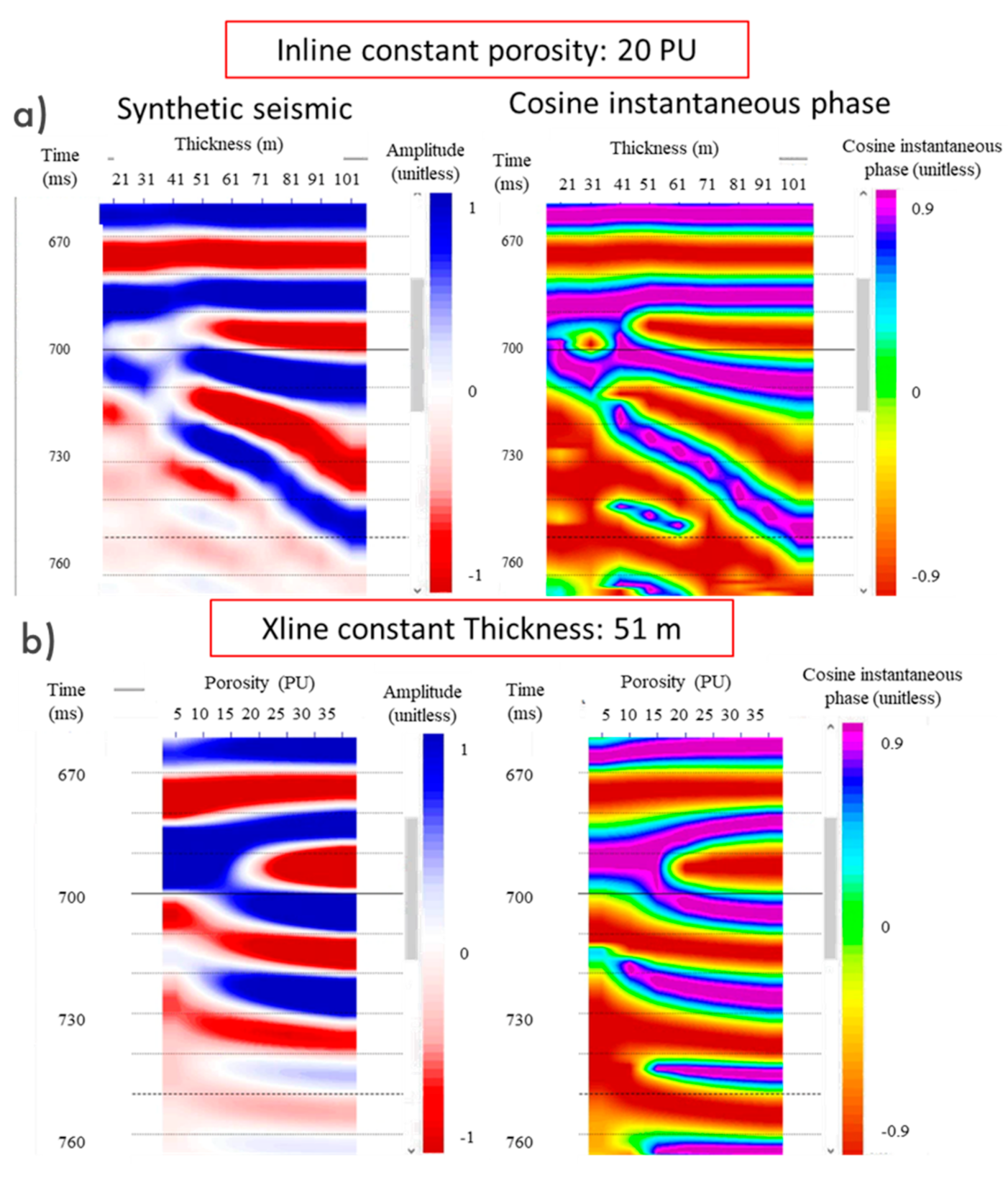
To understand why the cosine of the instantaneous phase is always chosen at the top of the multi-attribute list and why other phase attributes make at least half of the list when using Groups 3 and 4, a synthetic 3D volume was modeled in which the inline variations represent porosity from 5 to 35 porosity units (PU) at the 5-PU interval. The crossline variation represents thickness from 1 to 101 m at the 10-m interval. This is to evaluate the effect of porosity and thickness changes on the seismic phase response.

Figure 6a shows the amplitude and cosine of the instantaneous phase variations with thickness for an inline of the constant porosity of 20 PU. Figure 6b shows such variations with porosity for a crossline of the constant thickness of 51 m.

Figure 6 indicates that amplitude and cosine of the phase vary regularly with changing porosity or thickness.

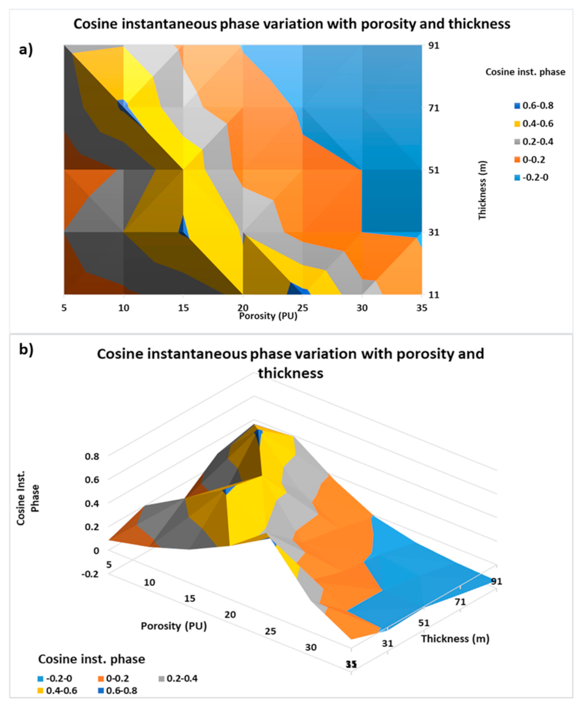
To better illustrate such changes, Figure 7 shows a surface plot in which the x-axis represents porosity, the x-axis represents thickness, and the color is the cosine of the instantaneous phase from the previously described synthetic model for a constant time sample at 700 ms from the synthetic cube. The pattern of almost linear and parallel lines of the constant phase indicates systematic cosine of the instantaneous phase sensitivity to porosity and thickness, thereby explaining why the seismic phase can be useful in rock properties prediction. In addition, phase has the advantage of being less affected by overburden attenuation and transmission losses than amplitude, making it possibly more robust in relating the seismic response to the layer impedance variations than amplitude. This a potentially important advantage of phase over amplitude in quantitative analyses of seismic data for rock properties prediction.

Figure 7 shows a plot that represents cosine instantaneous phase variations with porosity.

3.5. Porosity Prediction

In this study, the Hampson-Russell EMERGE software package is used to perform the multi-attribute prediction. The objective is to model the relationship between porosity logs and seismic attribute traces at well locations, and to predict a porosity volume with this relationship by predicting porosity from traces at other locations.

The following process was applied separately for each attribute group to obtain a different predicted porosity volume for each group of attributes.

• To stabilize the prediction, porosity logs were filtered to 100 Hz.

An initial multi-attribute list was generated to test convolutional operators with lengths from 1 to 51 samples incremented at every 10 samples and with a time sample rate of 1 ms. The operator length of 41 samples achieved the lowest validation error in all cases.

Figure 8 shows the resulting validation error versus the number attributes used in the regression.

2.

Out of the 24 available wells, 21 were used for training the algorithm and 3 were left as out-of-sample tests for blind validation.

3.

The transformation for each group was obtained using a 41-point operator length (representing 40 ms) and the attributes in Table 1.

Figure 9 shows the measured and predicted porosity logs, filtered to 100 Hz, for one validation well. Group 4 attributes generally gave the best porosity prediction (quantified below).

4.

Cross-validation among the training wells using the procedure described by Hampson [1] was used to restrict the number of attributes employed to 15.

5.

Porosity volumes were built. Figure 10 shows an inline of the predicted porosity for each volume. The inserted curve is a porosity log filtered to 100 Hz from one validation well and the color background of the curve represents the filtered porosity log colored to the same scale as the volume. Notice a tradeoff between matching the well logs and lateral stability of the predictions.

Average porosity maps over a 20-ms window below the seismic pick for the top of the most important reservoir layer were extracted to compare to interpolated average porosities from logs over the same window. Figure 11 shows average porosity maps for predictions made using the four attribute groups.

Maps were obtained by horizon-slicing porosity volumes. Black dots are well locations. Although all maps in Figure 11b–e follow a similar general trend, when compared to the interpolated porosity map from the logs (Figure 11a), Group 1 fails to accurately predict average porosity at well locations. The other three maps better match values from logs but away from well control, they behave differently. The ones from Groups 3 and 4 show more lateral heterogeneity and apparently sharper detail that could represent geological variation or could be due to seismic noise or numerical instability. Choosing between these explanations is an interpretive judgment, keeping in mind that Group 4 has the best accuracy at validation wells, as will be shown in the next section.

To better observe possibly geological behavior, Figure 12 shows a zoomed-in version of the map of average porosity obtained by using attributes in Group 4 indicating possible channels in a lacustrine fan-delta environment; being more channelized to the north and northeast and more delta front and fan-like in the center and to the south.

3.6. Accuracy and Statistical Significance of Results

The previous section explained the process followed to model and predict volumes and porosity maps. It also qualitatively compared the results obtained with the four at-tribute groups. In this section, statistical measures are implemented to determine the most accurate and statistically significant groups of attributes.

The predicted porosity logs versus actual porosity logs filtered to 100 Hz (Figure 13) were cross-plotted with only data from blind wells that were not included in the training process.

Table 2. R, mean absolute error (PU), standard error, F, and Significance F for actual versus predicted porosity logs for only the wells not used in the training process.

Validation	Group 1	Group 2	Group 3	Group 4
Correlation Coefficient	0.64	0.7	0.76	0.79
Mean Absolute Error	1.68	1.62	1.42	1.4
Standard Error	2.27	2.12	1.91	1.82
F	395	542	788	941
Significance F	5.57 × 10−67	2.36 × 10−84	8.90 × 10−109	7.31 × 10−122

gives the resulting values of the correlation coefficient between the measurements and predictions, mean absolute error, standard error, F (Fisher’s F-test), and significance F as measures of the regression statistical significance for each case.

Figure 13 shows cross-plots of the predicted versus actual porosity for all attribute groups’ predictions.

The correlation coefficient (R) is a measure of the degree to which the observation and prediction vary linearly rather than being a direct measure of accuracy. Mean absolute error (MAE: the arithmetic average of absolute errors) measures the aver-age magnitude of discrepancy between pairs of predicted versus observed values. MAE is expected to be as small as possible. However, as the sign of the error is lost in the magnitude, it does not reveal bias. It indicates precision better than accuracy.

To evaluate accuracy and bias, the standard error of the predicted mean is used. F is the ratio of the predicted variance to the error variance adjusted for the degrees of freedom (one less than the number of data points minus the number of attributes). When the ratio is less than 1, it can be concluded that the prediction is not useful. Significance F gives the probability that the correlation of the prediction and observation is a result of random chance [16]. A value below 0.05 is usually interpreted to mean the prediction is statistically significant. From Table 2, we can conclude that all the predictions are statistically significant, with bias and precision both being about two porosity units, approaching the accuracy of the logs. Compared to the measured log porosity, Group 4 has the best correlation, accuracy, and precision. Adding spectral decomposition to conventional attributes (Group 3) results in better incremental improvement compared to adding only relative geologic age (Group 2).

From Table 2, the correlation coefficient increases from 0.64 (Group 1) to 0.79 (Group 4). F is much greater than 1 and Significance F is virtually zero for all cases, which indicates that none of the models provides a spurious correlation (a correlation by random chance) of the predicted versus actual porosity. All the statistics improve systematically from Group 1 to Group 4.

Table 2 was calculated with point-by-point predicted-versus-actual porosity pairs for about 200 ms of data per well, spanning a larger interval than the main reservoir. For reservoir volumetrics, the porosity variation with depth (or seismic record time) is less significant than the average porosity over the reservoir interval. Figure 14 shows actual vs. predicted average porosity plots over reservoir interval.

For predicting the average porosity of the interval (

Table 3. Correlation coefficient and mean absolute error (PU), standard error, F, and Significance F for the actual versus predicted average porosity over a 20-ms window below the main reservoir.

Average Porosity	Group 1	Group 2	Group 3	Group 4
Correlation Coefficient	0.4	0.5	0.65	0.73
Mean Absolute Error	2.11	1.81	1.7	1.33
Standard Error	1.86	1.83	1.59	1.39
F	0.83	1.55	8.29	17.11
Significance F	3.70 × 10−01	2.20 × 10−01	9.20 × 10−03	5.11 × 10−04

), there is a more significant systematic improvement in statistics from Group 1 to Group 4, with correlation and statistical significance increasing and prediction error decreasing. The poor correlations for Group 1 and Group 2 have a significance of F greater than 0.05, which usually indicates that the correlation is not statistically significant. Such comparisons suggest that attribute Groups 3 and 4 are particularly important for accurately predicting average porosity at the reservoir level.

3.7. Resolution

The limit of vertical resolution (λ/4) is 10.04 m for the spectrally broadened seismic data used as input for this study.

Figure 15 shows thin hydrocarbon-bearing intervals evidenced on gamma-ray and resistivity logs, as well as associated porosities for a blind validation well that was not included in the training process.

All highlighted intervals in Figure 15 are at or above the limit of vertical resolution for the input bandwidth-extended seismic data. The four groups can detect such layers but only Groups 3 and 4 can accurately predict log porosities in them above 30 PU. The lowest reservoir just above a record time of 900 ms (black ellipse in Figure 15) is best detected by Group 4.

The Group 4 porosity volume is also useful to identify geologic features not seen on the seismic sections alone.

Figure 16 shows examples of channel-like bodies evident on the Group 4 predicted porosity volume that are not obvious on the original seismic data.

High porosity features on the right of Figure 16 resemble incised and stacked-high porosity channels. This response is expected in the area given that the reservoirs are fluvial and are lacustrine fan delta deposits. These features are imperceptible or are not clearly defined on seismic sections on the left.

Another example is shown in Figure 17. In this case, one well passes through the channel-like feature. Porosity and gamma-ray logs are shown, as well as the corresponding seismic section.

The computed porosity section in Figure 17 shows a high porosity possible channel and this interpretation is supported by well log porosity and gamma-ray responses, which indicate a very porous clean sand. The blocky shape of the sand layer suggests that the interval may correspond to a fluvial or deltaic distributary channel. The feature is about 10 m thick at the limit of seismic resolution and it is not obvious on the spectrally broadened seismic section. Thinner sand intervals are not resolved by the predicted porosity volume.

4. Discussion

Spectral broadening outside the original band of the seismic signal is controversial [6]. In the present study, the spectrally broadened seismic data is considered as an attribute: an arbitrary mathematical transformation of a seismic trace. Although Liang and Castagna [6] discussed under what circumstances such broadening can be viewed as physically accurate, Mora et al. [2] showed—for the same area in the Daqing field—that multi-attribute analysis of spectrally broadened data resulted in better predictions of well log porosity by all measures compared with a similar analysis with the original conventional seismic data. Based on the results, the spectrally broadened data is a significant input for multi-attribute analysis as indicated by cross-validation and blind well tests. The significance of the attribute was demonstrated by ties to well data and the performance in predicting porosity in both the training and validation [2], rather than by theoretical argument.

The attributes were derived from spectrally broadened seismic data and classified into four groups: conventional attributes (Group 1), conventional attributes and relative geologic age (Group 2), conventional attributes and components of spectral decomposition (Group 3), and all attributes combined (Group 4). Then, stepwise regression was performed for the attributes in each group to create a multi-attribute list that included the ten attributes within each group that yielded the best prediction error.

From the attributes included in the stepwise regressions, the cosine of the instantaneous phase was selected as the most significant attribute in all the cases, followed by relative geologic age when available. For Groups 3 and 4, more than half of the selections by stepwise regression were phase attributes. The high ranking of relative geologic age on the attribute lists is related to its ability to pinpoint where in a stratigraphic sequence a particular layer occurs, thereby taking advantage of any geologic succession in rock properties that may be learned in training. Conversely, the selection of the cosine of the instantaneous phase first in all the cases was an unexpected outcome, as it was the stepwise regression process that selected many phase attributes among the top 10 attributes.

The relationship between phase and porosity is explained with a synthetic wedge model (Figure 6 and Figure 7), showing that phase is sensitive to porosity and thickness in seismically thin layers. The isophase trends in the cross-plots of phase versus porosity and thickness suggest that the seismic phase response is related to the phase of the series of reflection coefficients for a given thickness. In addition, this is directly related to reservoir porosity through layer impedance. In synthetic data, the cosine of the instantaneous phase varies systematically with the porosity at a given time thickness. This relationship is particularly relevant in the present study that focuses on porous, thin, and discontinuous reservoirs. The cosine of the instantaneous phase removes all amplitude information that could be ambiguous in predicting porosity in thin layers and with overburden effects. As a result, the seismic phase potentially is more readily correlated to porosity than amplitude alone in thin layers. For this reason, it is understandable from a physical perspective that the attribute is selected first by stepwise regression and that the other phase attributes are also selected. The agreement between the predicted and actual porosity increases from Group 1 to Group 4. This is particularly true at the main reservoir level (blue rectangle in Figure 9 and dashed line in Figure 10), in which the highly porous interval is better predicted with the 10 attributes selected from all available attributes (Group 4). From Figure 10, the porosity seismic sections for all groups match the validation porosity log to some extent. The Groups 1 and 2 sections show continuous layers of the same porosity, while predicted porosity sections from Groups 3 and 4 show layers with great lateral variability. This last behavior is typical of a fan delta depositional environment. When comparing average porosity at the main reservoir level (Figure 11), Groups 2 to 4 seem to follow the same trend as the interpolated well logs. However, the Group 4 map shows more apparent detail and features that are possibly small channels (Figure 12). The areal extent of the predicted porous reservoir appears greatest for Group 4.

When compared to well logs, the porosity predicted with attributes in Group 4 shows more significant detail and is quantitatively closer to the measured porosity. The resulting metrics from the blind-well validation data not included in the training process (Table 2) show that Group 4 predictions are more accurate, more precise, and most statistically significant, with the highest correlation coefficient and F-value, as well as the lowest absolute and standard errors and lowest Significance F. Adding only relative geologic age (Group 2) increases the correlation coefficient and decreases error relative to Group 1. Adding only spectral decomposition components to the conventional attributes (Group 3) increases the accuracy and statistical significance of the prediction.

The differences in the metrics between the groups are more drastic when predicting average porosity at the reservoir level (Table 3), with a smaller error and both an increased correlation coefficient and statistical significance for the predictions made with Groups 3 and 4.

Figure 15 shows a comparison of the measured and predicted porosity at one well location used in the validation, in which three intervals of thicknesses that are barely above the λ/4 of 10.04 m are highlighted. The Group 3 and 4 predictions can better resolve these thin layers and the predicted values are closer to the actual values as compared to the predictions made with Groups 1 and 2.

The Group 4 predicted porosity volume can also be useful in identifying and delineating geological features of interest. Figure 16 shows three examples of channel-like features with high predicted porosity. It also shows a comparison to the corresponding spectrally broadened seismic section in which the same features are not obvious. Figure 17 shows a similar predicted high porosity penetrated by a well in which the logs validate the porosity prediction and channel interpretation.

5. Conclusions

Resolving thin layers of interest and predicting the rock properties variation in layers away from the well control are fundamental requirements in seismic reservoir characterization. In the present study, both problems were addressed by applying a combination of bandwidth extension, multi-attribute analysis, and non-conventional attributes to produce predicted porosity volumes for a portion of the Daqing field in China. The attributes were derived from spectrally broadened seismic data and multi-attribute analysis was implemented with four groups of attributes separately. Group 1 is comprised of conventional attributes. Group 2 is comprised of conventional attributes and relative geologic age. Group 3 is comprised of conventional attributes and spectral decomposition components including amplitude, magnitude, phase, and the cosine of the phase at 10 Hz increments. Group 4 is comprised of all the attributes listed prior.

The result presents the comparison of the resulting resolution, accuracy, and statistical significance of multi-attribute rock properties prediction for each group. It was observed that the geometries of the predicted porosities was geologically reasonable for the fan delta environments responsible for depositing the thin reservoir sandstones in the Daqing field. Group 1 gave the least accurate predictions. In contrast, the predictions with both spectral decomposition volumes and the relative geologic age gave the best performance by all the metrics. Phase attributes improved porosity prediction despite their independence from the seismic amplitude.

The results show that combining spectrally broadened seismic data and multi-attribute analysis with non-standard seismic attributes can be a powerful approach for resolving, delineating, and characterizing reservoirs at or below the limit of conventional seismic resolution.

References

1. Hampson, D.; Quirein, J.; Schuelke, J. Use of multi-attribute transforms to predict log properties from seismic data. Geophysics 2001, 66, 220–236. [Google Scholar] [CrossRef]
2. Mora, D.; Castagna, J.; Meza, R.; Chen, S.; Jiang, R. Case study: Seismic resolution and reservoir characterization of thin sands using multi-attribute analysis and bandwidth extension in the Daqing field, China. Interpretation 2020, 8, T89–T102. [Google Scholar] [CrossRef]
3. Ray, A.; Biswal, S. An efficient method of effective porosity prediction using an unconventional attribute through multi-attribute regression and probabilistic neural network: A case study in a deep-water gas field, East Coast of India. SEG Tech. Program. Expand. Abstr. 2010, 2021, 1413–1417. [Google Scholar]
4. Abdulaziz, A. The effective seismic attributes in porosity prediction for different rock types: Some implications from four case studies. Egypt. J. Pet. 2020, 29, 95–104. [Google Scholar] [CrossRef]
5. Zhang, R.; Castagna, J. Seismic sparse-layer reflectivity inversion using basis pursuit decomposition. Geophysics 2011, 76, 147–158. [Google Scholar] [CrossRef] [Green Version]
6. Liang, C.; Castagna, J.; Zavala, R. Tutorial: Spectral bandwidth extension—Invention versus harmonic extrapolation. Geophysics 2017, 82, w1–w16. [Google Scholar] [CrossRef]
7. Ryder, R.; Quiang, J.; McCabe, P.; Nuccio, V.; Persits, F. Qingshankou-Putaohua/Shaertu and Jurassic Coal—Denglouku/Nongan Total Petroleum Systems in the Songliao Basin, China; U.S. Geological Survey: Reston, VA, USA, 2003. [CrossRef]
8. Puryear, C.; Castagna, J.; Portniaguine, O.; Cobos, C. Constrained least-squares spectral analysis: Application to seismic data. Geophysics 2012, 77, V143–V167. [Google Scholar] [CrossRef]
9. Chen, S.; Donoho, D. Basis pursuit. In Proceedings of the 1994 28th Asilomar Conference on Signals, Systems and Computers, Pacific Grove, CA, USA, 2 November 1994; pp. 41–44. [Google Scholar]
10. Taner, M.; Schuelke, J.; O’Doherty, R.; Baysal, E. Seismic attributes revisited. In SEG Technical Program Expanded Abstracts; Society of Exploration Geophysicists: Tulsa, OK, USA, 1994; pp. 1104–1106. [Google Scholar]
11. Barnes, A. The complex seismic trace made simple. Lead. Edge 1998, 17, 473–478. [Google Scholar] [CrossRef]
12. Chopra, S.; Marfurt, K. Seismic attributes—A historical perspective. Geophysics 2005, 70, 3SO–28SO. [Google Scholar] [CrossRef]
13. Barnes, A. A tutorial on complex seismic trace analysis. Geophysics 2007, 72, W33–W43. [Google Scholar] [CrossRef]
14. Stark, T. Relative geologic time (age) volumes—Relating every seismic sample to a geologically reasonable horizon. Lead. Edge 2004, 23, 817–944. [Google Scholar] [CrossRef]
15. Russell, B.; Hampson, D. Multi-attribute seismic analysis. Lead. Edge 1997, 16, 1439–1444. [Google Scholar] [CrossRef]
16. Mathews, S. Interpreting Regression Output—Without all the Statistics Theory. 2018. Available online: https://www.graduatetutor.com/statistics-tutor/interpreting-regression-output (accessed on 5 May 2021).
Figure 1. (a) Location of the seismic survey. Black dots represent the relative location of 24 wells. (b) Inline of spectrally broadened volume. The yellow horizon represents the top of the reservoir interval.
Applsci 11 08034 g001
Figure 2. Amplitude spectrum of spectrally broadened data.
Applsci 11 08034 g002
Figure 3. Well-tie to spectrally broadened data; the correlation coefficient is 0.75. Red trace: composite seismic trace. Blue trace: synthetic trace. The right side shows the statistical wavelet used. Polarity: an increase in amplitude corresponds to an increase in acoustic impedance.
Applsci 11 08034 g003
Figure 4. Inline example of relative geologic age volume. Each color represents a different seismically inferred relative geologic age.
Applsci 11 08034 g004
Figure 5. (a) Amplitude at 100 Hz (polarity: an increase in amplitude corresponds to an increase in acoustic impedance), (b) magnitude at 100 Hz, and (c) phase at 100 Hz.
Applsci 11 08034 g005
Figure 6. (a) Left: inline of synthetic seismic data that represents constant porosity of 20 PU; crossline variations represent thickness changes. Right: cosine of the phase of the inline on the left. (b) Left: crossline of synthetic seismic data that represents a constant thickness of 51 m; inline variations represent porosity changes. Right: cosine of the instantaneous phase of the crossline on the left. Polarity: an increase in amplitude corresponds to an increase in acoustic impedance.
Applsci 11 08034 g006
Figure 7. Cosine of the instantaneous phase variation at 700 ms for porosity versus thickness wedge models. (a) Crossplot view and (b) 3D view.
Applsci 11 08034 g007
Figure 8. Average training error versus the number of attributes testing convolutional operator lengths from 1 to 51 samples every 10 points. The black arrow indicates the point of the lowest validation error achieved using a 41-point operator. The example shown corresponds to the Group 4 attribute selection process. As the sample rate is 1 ms, the 41-point operator represents 40 ms.
Applsci 11 08034 g008
Figure 9. Comparison of resulting predicted log (red) and actual porosity log filtered to 100 Hz (black) for a well not used in the training process using the different attribute groups. Error is the mean absolute error over the prediction interval. The blue rectangle highlights the main reservoir unit. A small time–depth error at the reservoir level is more obvious for Groups 3 and 4.
Applsci 11 08034 g009
Figure 10. Inline of the predicted porosity volume obtained using each of the attribute groups. The inserted curve is a porosity log filtered to 100 Hz from one validation well and the color background of the curve is the log colored to the same scale as the volume. The dashed black line indicates the top of the main reservoir. Abbreviation: SD, spectral decomposition.
Applsci 11 08034 g010
Figure 11. (a) Interpolation of the average porosity over a 20-ms window below the main reservoir top shown in Figure 10. (b) Group 1 map of average porosity over a 20-ms window below the main reservoir seismic pick in Figure 10. (c) Group 2 map of average porosity over a 20-ms window below the main reservoir seismic pick shown in Figure 10. (d) Group 3 map of average porosity over a 20-ms window below the main reservoir seismic pick shown in Figure 10. (e) Group 4 map of average porosity over a 20-ms window below the main reservoir seismic pick shown in Figure 10.
Applsci 11 08034 g011
Figure 12. Map of average porosity over a 20-ms window below the main reservoir top. The map was obtained by slicing the porosity volume from Group 4. Black dots are well locations. The black circle highlights an example of what could be channel-like features in a fan-delta environment.
Applsci 11 08034 g012
Figure 13. Cross-plots of the actual versus predicted porosity for predictions made using each of the attribute groups in three blind validation wells. Abbreviations: CC, correlation coefficient and MAE, mean absolute error. Data from the entire length of available logs were used in this cross-plot.
Applsci 11 08034 g013
Figure 14. Cross-plots of the actual versus predicted average porosity extracted over a 20-ms window below the main reservoir. Abbreviations: CC, correlation coefficient and MAE, mean absolute error.
Applsci 11 08034 g014
Figure 15. Thin hydrocarbon-bearing intervals seen on logs and predictions made using the four attribute groups. The inserted curve is a porosity log filtered to 100 Hz. The well shown was not used for training. Black ellipse highlights a reservoir of interest, most detectable using Group 4 prediction.
Applsci 11 08034 g015
Figure 16. Right: sections from the Group 4 porosity volume showing channel-like features. Left: same sections from the seismic volume used as input for multi-attribute analysis. Polarity: an increase in amplitude corresponds to an increase in acoustic impedance.
Applsci 11 08034 g016
Figure 17. From left to right: porosity and gamma-ray log. Group 4 predicted porosity volume, with a red line indicating the well path, corresponding to the spectrally broadened seismic section. The blue rectangle highlights the channel-like feature. Polarity: an increase in amplitude corresponds to an increase in acoustic impedance.
Applsci 11 08034 g017