Abstract
The paper briefly presents the dynamic synthesis of mechanisms with superior couplings, force, and speed distribution, efficiency, loss coefficient, dynamic coefficient or motion transmission function, determination of variable angular input speed from the crank or cam based on solving the equation Lagrange, the determination of the dynamic variation of the follower (adept) based on the integration of Newton’s equation, and the dynamic analysis of several models taken into account. In the end, the original relations for calculating the efficiency of a gear are presented.
1. Introduction
The mechanisms with superior couplings are generally the most used; they have the advantage of a superior, irreversible transmission, with the movement from element 1 transmitted to element 2 being different from the movement transmitted from element 2 to element 1. These superior couplings are made on a point or a line but never after a surface, as is the case with inferior and reversible couplings.
The most used upper couplings are those with cam and follower, flat or spatial, and the gears. Rarely, there are also superior couplings such as the Maltese cross mechanism (Geneva driver), the ratchet mechanism, etc.
Throughout its history, the Department of Theory of Mechanisms and Robots at the Polytechnic University of Bucharest, Romania, has enjoyed the activity and presence of distinguished professors and researchers such as N.I. Manolescu, a corresponding member of the Romanian Academy, 16 years in a row (four consecutive terms) as dean of the Faculty of Transport 1957–1972, founder of ARoTMM (Romanian Association for Theory of Mechanisms and Machines), which requested the establishment of IFToMM, and signed from Romania the founding document of IFToMM (International Federation for Theory of Mechanisms and Machines) in 1969, ten years as head of the Department of Theory of Mechanisms 1962–1972 (consulting professor during 1973–1993).
At the express request of (Corresponding Member of the Romanian Academy, University Professor doctor of science and engineering) Nicolae I. Manolescu, then head of the Department of Theory of Mechanisms at the Polytechnic University of Bucharest, representatives from 13 states gathered in the fall of 1969 in Poland, in Zakopane, to establish (Fonda) the International Federation for Theory of Machines and Mechanisms (IFToMM); it was decided on this occasion that all participating states to start the establishment of national associations to be subordinated to the IFToMM. Some of the great teachers of the time gave names to various types of mechanisms, some of which were not sufficiently addressed, and because of this, their names or definitions have been lost or confused with other types of mechanisms, today. This is the case of the name of mechanisms with rigid memory, as it was defined by NI professors Manolescu, and others at that time.
The Romanian school of mechanisms, the one that proposed the establishment of IFToMM, kept the name and definitions of the mechanisms of that time, among which is that of the mechanisms with rigid memory, these being mechanisms with superior couples that can only be operated from element 1 towards element 2 and not the other way around, as is the case with mechanisms with superior coupling, as cam-follower.
In this old conception, rigid memory mechanisms are those mechanisms that are operated only from the driving element of the coupling, the reverse of which cannot be possible. A valve mechanism will only be able to operate when the stopper or pusher actuates the valve, and not the other way around, because being actuated from the valve will lock. In cam-dash systems (Figure 1), the cam is always the driving element, and the tappet is the driven element, and if you try reversing the driving element so that the follower introduces movement, the mechanism will lock and will not work.
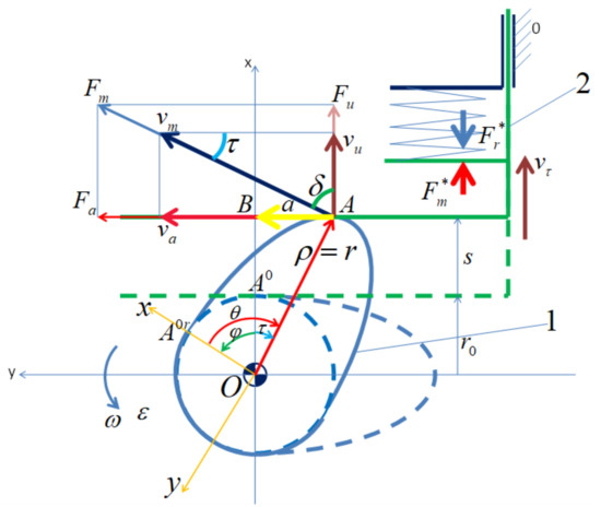
Figure 1.
A mechanism with rotary cam and a plate, translated tappet.
The rotating cam 1 actuates the follower 2 in translational motion, conversely, the movement being impossible, i.e., the follower 2 will not be able to actuate the cam 1 because the mechanism will lock immediately. In Figure 1, the cam rotates in a trigonometric direction, considered positive, counterclockwise. From a dynamic point of view, the movement in a superior couple tends to align with the forces in the couple, so the dynamic (real) speeds imposed on the follower by the cam will have the same directions as the similar forces that produce them. The authors of this paper have established, by this simple and original rule, a new dynamic of the mechanisms with superior torques. The new rule can be successfully applied and generalized to all types of mechanisms, with it being tested by authors on engines, mechanical transmissions, and many other mechanisms, with great success. The new idea imposed by the authors is a simple one. The driving force Fm produced by the driving element 1, in this case, the cam, is always perpendicular to the position vector (r) of the contact point A, between the cam 1 and the follower 2, and directed in the direction of movement, and rotation, of the cam 1. The motor force is always known, being a value, with the known motor moment divided by the length of the vector r. The motor speed vm is produced by the driving force and acts in the same direction and sense as the driving force. It is also known to be equal in value to the product of the vector r and the angular velocity ω of cam 1. The driving force Fm is divided into the useful force Fu acting directly on the follower and the slip or loss force Fa. The speeds are positioned similarly to the respective forces. The pressure angle here is delta (δ), while the transmission angle is tau (τ).
The same happens with the systems formed by a Maltese cross and a leading element with one or more inputs (Figure 2), where the cross is always the driven element, and if an attempt is made to reverse the command and turn the cross into a conducting element, the coupling would crash immediately.
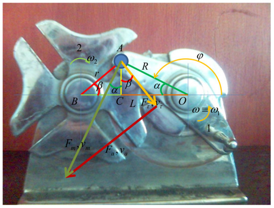
Figure 2.
A Geneva driver mechanism.
The leading element 1 (here with two inputs) operates the driven element 2, the cross, conversely with the movement, is not possible, i.e., the cross 2 will not be able to operate element 1 because the mechanism will lock immediately. The conductive element 1 has a bolt that pushes into the wall of the cross canal to operate it. The driving force Fm acts at the point of contact A and is perpendicular to the vector R, it being known and having the value of the motor moment of the element 1 divided by the radius R. The driving force Fm will generate a useful or transmitted force Fτ and a loss or slip force Fa. The useful force acts perpendicular to the wall of the cross channel, while the slip occurs along the cross channel. The pressure angle here is delta (δ) (=alpha plus beta), while the transmission angle is tau (τ) (=pi/2 − alpha − beta = π/2 − δ). The speeds are similar to the forces that determine them.
Mechanisms of this kind have been used for hundreds of years in automation, control, actuators, mechanical transmissions, robots, energetics, automobiles, and vehicles, in household appliances, and in general throughout the industry. In automatic machines but also in cars or other vehicles, especially in engines, these mechanisms must withstand very high loads and speeds for a long time for a huge number of cycles, for which they must achieve a dynamic operation silently, normally, and without major noxious substances, vibrations, noises, interruptions, blockages, imbalances, or large variations of the angular speed. The dynamic conditions imposed on mechanisms with superior couples are drastic, and they cannot yet be replaced with coils or other mechanisms. The huge resistance achieved by the mechanisms with superior couples has definitely established them, even if they used to work with low mechanical efficiencies.
The study of the dynamics of these mechanisms will be presented briefly in this paper, in an original unitary vision.
It is the merit of the German engineers Eugen Langen and Nikolaus August Otto to build (physically, practically, the theoretical model of the Frenchman Rochas), the first internal combustion engine in four strokes, in 1866, with electric ignition, carburetion, and distribution in an advanced form. The distribution mechanisms of today are identical to those of that time, but they have acquired several valves per cylinder in order to be able to achieve a naturally variable distribution. In 1889, Daimler improved the four-stroke internal combustion engine by building a “two-cylinder V”, and bringing the distribution mechanism to its classic shape, “with mushroom-shaped valves” [1].
In 1892, the German engineer Rudolf Christian Karl Diesel, invented the compression ignition engine and fuel injection or, in short, the diesel engine. The first diesel engines were designed (even by design) to run on biofuels. Thus, the first model presented by Diesel worked with squeezed vegetable oil from hazelnuts (peanuts).
Later it was adapted to diesel, which could not be used in gasoline engines because diesel had too low of an octane number, and the Otto engine (then with carburetion and spark ignition) was self-igniting, as it does today when fuels used do not have a high octane number. Only two-stroke carburetor (fuel mixture) engines can cope with heavier fuels, i.e., petrol and mixtures with a lower octane number, but they also get dirty very quickly with diesel. Additionally, they also start to ignite. Diesel, with a low octane number, is perfect for diesel fuel injection and self-ignition engines, as well as many vegetable oils. It should also be noted that diesel engines remove the carburetor from the start by compressing only the air, the fuel being introduced when the compression is finished, by injection and spraying (spreading) under pressure. It ignites immediately due to high pressures (due to air compression). By burning it, the temperature increases significantly, which further increase the pressure in the combustion chamber producing the engine time (expansion). Today, Otto engines also removed carburetor, injecting fuel like diesel engines, but they still use spark plugs to ignite the fuel by a spark. In general, the Delco has been replaced with electronic ignition. Diesel engines also have an ignition system that works only in cold, i.e., only when starting the engine cold, after which it automatically shuts off [1].
The first valve mechanisms appeared in 1844, being used for steam locomotives; they were designed and built by the Belgian mechanical engineer Egide Walschaerts.
The first cam mechanisms are used in England and the Netherlands in weaving wars. In 1719, in England, a certain John Kay opened a spinning mill in a five-story building. With a staff of over 300 women and children, and this would be the first factory in the world. He also became famous for inventing the flying shuttle, due to which the tissue becomes much faster. The cars, however, were still manually operated. It was not until around 1750 that the textile industry was revolutionized by the widespread application of this invention. Initially, the weavers opposed him, destroying the flying sparks and driving out the inventor. Around 1760, weaving wars and the first factories in the modern sense of the word appeared [1].
Hren and his team analyze the load moments on several models of the classic mechanisms with superior couples. A method of creating dependence on the ratchet stroke has been developed. The stroke dependence is generated based on the desired stroke of the polynomial degree and the connection angle of the cam profile on the base circle. The degree of the polynomial is expressed by an odd natural number. The release method was expressed by the normal force between the cam and the stud. Then, the stroke and the required moment were determined. What is given a higher degree polynomial is a requirement for the minimum radius of the larger basic theoretical circle [2].
Many current concerns regarding cam-follower mechanisms and their optimal dynamics relate to their use in automatic machines and industrial processing [3,4,5,6,7,8,9,10,11].
Normally, in a system with cam and follower the cam is operated at a constant speed while the movement of the dowel is imposed by the curve belonging to the cam profile. Kinematically, it is possible to improve the movement of the tracker by varying the input speed of the cam. Various polynomial laws of motion are studied in order to determine theoretically and experimentally their influence on the motion imposed on the stem by the cam. It is desired to design an optimal path of the ratchet for a certain angular speed of the cam. Design examples are provided to illustrate the procedure for obtaining a suitable speed trajectory as variable speed cam tracking systems. Moreover, an experimental configuration with a servo controller is developed to study the feasibility of this approach [12].
Gatti and Mundo approach a preliminary study on the control of followers ‘vibrations in followers’ mechanisms when acting directly on the follower. Due to the elasticity of the mechanical components, the movement of the follower is affected by unwanted dynamics, which can compromise its accuracy. Different techniques are commonly used to reduce such unwanted vibrations, but they approach the problem in an indirect way. The purpose of this paper is to investigate the feasibility of controlling the follower’s movement by applying a secondary force directly to it. To the extent that the authors are aware, there is no clear indication in the literature why such direct control has not been considered by researchers so far. Therefore, this paper intends to address the limits of such a control approach by giving the reader an even broader picture of this issue. Simple active and passive control strategies are investigated and compared. The simulations are performed only on the basis of “purely mechanical” considerations and alone draw an important conclusion about their effectiveness or practical feasibility [13].
The design of mechanisms with superior couples, especially when used in robots, has been a major concern for many authors [14,15,16,17,18,19,20,21,22,23,24,25,26,27,28,29,30,31,32,33,34,35,36,37,38,39,40,41,42,43,44,45,46].
Mechanisms with superior couples are increasingly used in medicine, medical equipment, control equipment, artificial hearts, pacemakers, prostheses, etc. [47,48,49,50,51,52,53,54].
This paper will present some basic aspects of the dynamics of the planar mechanisms with superior couples, such as dynamic operation, the variation of the angular velocity of the cam depending on its position, the yields of the mechanism, the transmission of forces, speeds, moments, equations of motion, solving the equations of movement, balancing, reduction in angular velocity variation, follower vibrations.
2. Materials and Methods
2.1. Geometric Synthesis
A rapid method of geometric synthesis is that of Cartesian coordinates (see Figure 1). In the fixed system xOy, the Cartesian coordinates of the contact point A (belonging to the block 2) are given by the projections of the position vector rA on the Ox and Oy axes respectively, and have the analytical expressions expressed by the relational system (1).
In the mobile system x’Oy’, the Cartesian coordinates of the contact point A (belonging to the profile of the cam 1, which rotated clockwise with the angle φ), are given by the relations of the systems (2) and (3) [1].
2.2. Distribution of Forces and Determination of Efficiency a Classic Mechanism with Rotating Cam and Translucent Flat Ratchet
The distribution of forces was first introduced by the author [1] and it does not refer to the determination of forces acting on a mechanism. The reactions in the mechanism known from the classical methods determine the forces acting in the torques of the mechanism and show the maximum loads in the mechanism, as well as the variation of the inertia forces in the respective mechanism. The method of determining the distribution of forces shows the way in which the forces act in couples, on elements, and especially the way in which they are transmitted from one element to another within the respective kinematic coupling. It is an original method that allowed, in time, the author to deduce the exact mechanical efficiency of the mechanisms, the dynamic coefficients in the mechanism, the variation of the forces acting in the mechanism, and new methods for deducing the dynamics of the mechanism in question.
Figure 3 analyzes the distribution of forces and velocities within a mechanism with superior couple with a rotating cam, ratchet, and classic translational movement, plane.
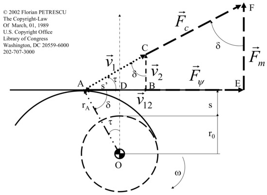
Figure 3.
Forces and speeds at the translated dept with the sole.
The main angles that appear in the mechanism are the pressure angle (delta) and the transmission angle (tau) both being in a relationship of complementarity.
The consumed motor force, Fc, perpendicular in A on the vector rA, is divided into two components: (a) Fm, which are the use force, or the reduced motor force at the dowel; (b) Fy, which is the sliding force between the two cam and dowel profiles, (see Figure 3) and relations (4)–(13) [1].
The efficiency of the mechanism (8), originally determined by the distribution of forces in the mechanism, can be expressed simply by the relation (8) either according to the transmission angle (tau) or according to the pressure angle (delta). The relationship indicates practically instantaneous mechanical efficiency. In order to determine the total mechanical efficiency, it is necessary to integrate on the whole working portion, ascent, and return.
It can be easily verified that the instantaneous loss added with instantaneous efficiency permanently gives the total value 1.
The way in which the dynamic coefficient D is expressed and determined is represented exactly (in more detail) in the paper [1], here being only exposed the relation (14) from which it is made explicit.
The dynamic coefficient of this type of mechanism or its transmission function, D, is determined by the relations (14), where D’ is the D derivative depending on the angle FI [1].
The speed based on the dynamic coefficient is expressed with the relation (15) and the corresponding acceleration is determined with the Equation (16), Figure 4 [1].
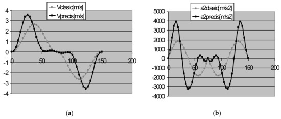
Figure 4.
Comparison between classical kinematics and proposed kinematics in this paper. (a)-speeds and (b)-accelerations of the ratchet.
Figure 4 shows the differences between known classical kinematics and precision kinematics introduced, for the first time, by the author in the paper [1].
The precision kinematics influenced by the dynamic coefficient, presents a slight dynamic aspect, due to the influence of the way in which the forces and speeds are transmitted within the mechanical coupling.
2.3. Approximate Solution of the Lagrange Equation of Motion
The exact dynamics of the mechanism are introduced with the support of the Lagrange equation of case I. The way in which the equation of motion of the car (Lagrange) is solved is completely original, and makes a great contribution to the study of machine dynamics. The method is presented for the classic distribution mechanism, where the cam is rotating and the flat adept is in translational motion. The method can be adapted to any type of mechanism, plane, or space. The Lagrange equation of type I, written in the differential form (also called the machine equation), has the form (17), where J* is the moment of inertia (mass, or mechanical moment) of the mechanism, reduced to the crank, and M* represents the reduced motor moment minus the reduced resistance moment, reduced to the crank (or cam); the angle φ represents the angle of rotation of the crank. J*’ represents the derivative of the mechanical moment as a function of the angle φ of rotation of the crank; [1].
We write relationships (18) and (19):
where Fr is the reduced resistance force, Fm is the reduced motor force, Mr is the reduced resistance moment at the crank or cam, Mm is the reduced motor moment at the crank or cam, and Equation (3) establish the shape of the Lagrange equation of motion originally solved in dω by authors [1].
The most important original part was the elimination of the two unknowns from a single equation, ω and eps, and the introduction of a single unknown dω, so that the differential equation was written in classical Lagrange form, now with a single unknown dω can be solved very easily and directly without requiring the use of various special numerical methods. So we must emphasize that the primordial originality consisted in replacing the two unknown dependencies variables ω and eps with a single independent variable dω.
Practically the variable ω was written to be equal to ωn + dω, where ωn represents the constant nominal value of the angular velocity depending on the speed of the camshaft, and dω is the small instantaneous variation of the angular velocity which depends on the FI position of the camshaft.
from the relational system (19) it can be seen that the angular acceleration eps = has been replaced by the expression ωdω/dFI, so that the second variable of the Lagrange equation eps disappears (it is in fact dependent on the first variable w and the instantaneous FI position of the camshaft). By this computational artifice, the two dependent variables ω and eps of the Lagrange equation are practically eliminated and replaced with a single variable, dω. In this way, the equation can be solved easily and directly without the need for the classical approximate numerical methods used. The originality of the solution takes over the classical tasks and transforms the approximate classical equation of motion into a simple 2nd-degree equation that admits real exact solutions easy to determine physically-mathematically.
Another novelty in the presented dynamic method is the way in which the dynamics of the follower is solved.
It should be noted here that the Lagrange equation already presented can only determine in the end only the variable rotational speed ω of the camshaft (cam). The complete dynamics of the cam and ratchet mechanism also requires the determination of the variable adept kinematics, i.e., its dynamic offset x, different from the law of motion imposed on the ratchet s, its dynamic speed x’ different from s’, and its dynamic acceleration x″ different from s″. The original Equations (20) and (21) used for this purpose were obtained by integrating the known classical Newtonian equation of motion. Those who want to know how to obtain the Equations (20) and (21) must study the paper in detail [1], because the calculations are long and tiring and there is no room here for their presentation. It is used to determine the dynamic displacement of the adept, the relations (20) and (21) [1].
After obtaining the real, dynamic displacement x of the follower, with the help of the original Equation (21), thus it will be derived twice in relation to time and in this way, the exact equations for determining the dynamic tappet speed x’ and of its dynamic acceleration x″ will be obtained (see [1]). Another original aspect is the comparison of the two known classic equations of motion of the machine, the first written in the form of Newton (22) and the second in the form of Lagrange (23) of type I.
By identifying the terms of Equation (22) Newton and (23) Lagrange, we obtain: reduced motor force (24), reduced resistance force (25), and variable damping coefficient c (26) [1]:
2.4. Swivel Cam Mechanisms and Translated Adept with Roll
Figure 5 shows a mechanism with rotating cam and adept with roller in translational movement. Turning to the mechanism with a rotating cam and a follower with roller in translational motion, the authors make important new contributions to mechanical systems with superior couples, among which could be listed a few: determining two angles of pressure for this type of mechanism; transmission of forces and speeds; determining the dynamic coefficients and the instantaneous mechanical efficiency; the exact theoretical realization of the dynamics of the mechanism, with the determination of the variable angular velocity of the cam w and of the variable dynamic displacement of the ratchet x; dynamic synthesis of the mechanism.
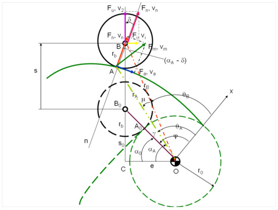
Figure 5.
A mechanism with rotating cam and adept with roller in translational movement.
The pressure angle δ, which appears between the normal n taken through the contact point A and a vertical, has the known quantity given by the relations (27)–(29):
We can also directly determine the angle αA (30) and (31):
The cam profile can now be drawn directly using the polar coordinates rA (known, see relation (9)) and θA (which is determined by relations (32)–(37):
One writes the following relations of forces and velocities (38)–(42) [1]:
Instantaneous yield is determined (16):
It can be seen that the instantaneous mechanical efficiency of this type of mechanism ultimately depends on the cosine of the classical pressure angle raised to the fourth power.
The transmitted dynamic forces have more complex expressions for this type of mechanism, which makes the dynamics more difficult and more complex.
2.5. Mechanism with Rotating Cam and Rotating Adept with Roller
Next, we try to follow, very briefly, the same parameters but for another type of mechanism with superior couple, namely of the one with a rotating cam and rotating rocker having a contact roller. Figure 6 shows a mechanism with rotating cam and rotating adept with roller. Within this mechanism, there are two different angles of pressure, the fact being practically due to the additional roller that is mounted on the stem. Basically, the appearance of the roller makes the classic delta pressure angle be doubled by a second constructive alpha pressure angle.
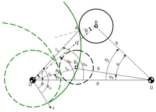
Figure 6.
A mechanism with rotating cam and rotating adept with roller.
Next, some kinematic parameters are determined, with the help of which the cam profile can be drawn directly, for the mechanism with rotating cam and roller rocker adept (43)–(50) [1].
The forces and speeds at the mechanism with rotating cam and rocker arm with a roller are determined by the relation (51), Figure 7 [1].
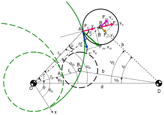
Figure 7.
Forces and velocities to a mechanism with rotating cam and rotating adept with roller.
The roller is responsible for differentiating the transmitted forces, because the classic cam-tappet coupling is actually replaced by a composite coupling which consists of two simple couplings, one between the cam and the roller and a second between the roller and the tappet. Even if the force Fa is a loss force, it has an important role in the mechanism, practically rotating the roller around its joint B, so that the contact changes permanently and the roller wears evenly and more slowly.
2.6. The Mechanism with Rotating Cam and Rotating Adept (Flat Rocker)
Figure 8 and Figure 9 show the mechanism with rotating cam and rotating adept (flat rocker). The calculation relationships will be summarized below (52)–(57) [1]:
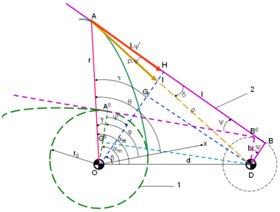
Figure 8.
A mechanism with rotating cam and rotating adept (flat rocker).
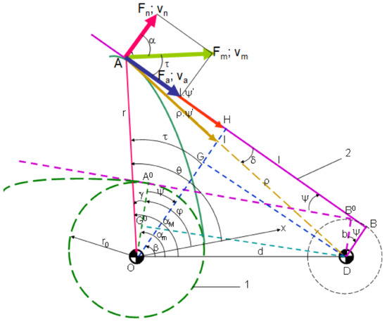
Figure 9.
Forces and velocities to a mechanism with rotating cam and rotating adept (flat rocker).
3. Results
The dynamic analysis of the classical law sine, is seen in the diagram in Figure 10, and in Figure 11, the one for an original law is observed (C4P):
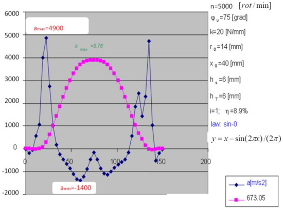
Figure 10.
Dynamic analysis of the law sin, φu = 75 [degree], n = 5000 [rpm], for the classic module with rotating cam and translation tracker with sole.
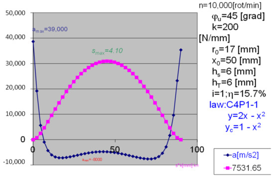
Figure 11.
Dynamic analysis of the law C4P, φu = 45 [degree], n = 10,000 [rpm], for the classic module with rotating cam and translation tracker with sole.
Below is presented the dynamic analysis of module B, for some known laws of motion. It starts with the classical law SINE (see the dynamic diagram in Figure 12), in order to be able to compare it with the dynamics of this law from the classical module C. It uses a speed of n = 5500 [rot/min], for a maximum theoretical displacement both at valve as well as at the dowel, h = 6 [mm]. The phase angle is, φu = φc = 65 [degree]; the radius of the base circle has the value, r0 = 13 [mm]. For the radius of the roller, the value rb = 13 [mm] was adopted. The eccentricity of the guide, relative to the center of the cam, is e = 6 [mm]. The yield has a high value, η = 11.5%; the spring settings are normal, k = 30 [N/mm] and x0 = 20 [mm]; where k is the elastic constant of the spring (valve) and x0 is the pre-tightening of the spring. We remind you that module B has a rotating cam and an adept with a translational movement with a roller.
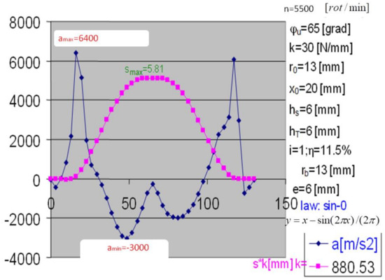
Figure 12.
Dynamic analysis at module B. SINE law, n = 5500 [rot/min] φu = 65 [degree], r0 = 13 [mm], rb = 13 [mm], hT = 6 [mm].
The dynamics is better (in general) compared to that of the classical module, C. For a phase angle of only 65 degrees, we reach the same acceleration peaks that the classical module reached at a relaxed phase of 75–80 degrees.
Figure 13 shows the corresponding profile, drawn inversely to those in module C, i.e., with the lifting profile on the left and the return profile on the right, (because the direction of rotation of the cam was also reversed, from schedule to trigonometric).
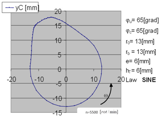
Figure 13.
Cam profile at module B. SINE law, n = 5500 [rot/min] φu = 65 [degree], r0 = 13 [mm], rb = 13 [mm], hT = 6 [mm].
For the cosine law, the vibrations are calmer compared to the sine law, as in the classical dynamic module, C (see the dynamic diagram in Figure 14).
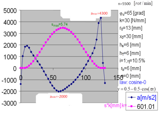
Figure 14.
Dynamic analysis at module B. COSINE law, n = 5500 [rot/min] φu = 65 [degree], r0 = 13 [mm], rb = 6 [mm], hT = 6 [mm].
The chosen speed is n = 5500 [rot/min], for a maximum theoretical displacement, both at the valve and at the rake, of h = 6 [mm]. The phase angle is, φu = φc = 65 [degree]; the radius of the base circle has the value, r0 = 13 [mm]. For the radius of the roller, the value rb = 6 [mm] was adopted. The eccentricity of the guide relative to the center of the cam is, e = 0 [mm]. A dynamic study shows that what is gained in efficiency in one of the phases (ascent or descent) due to eccentricity, e, is lost in the other phase, so that, e, can adjust one phase and at the same time deregulate the other. Here is a serious reason that its adopted value is zero. The efficiency of the mechanism has a high value (higher than that of the classical module, C), η = 10.5%, but lower by a percentage compared to the law sin. The spring settings are normal, k = 30 [N/mm] and x0 = 30 [mm]. The COSINE profile (for dynamic module B), corresponding to the dynamic diagram in Figure 14, is drawn in Figure 15. The profile of raising or ascending, or attacking, is the one on the left, and the one of return (or descent) is located on the right. As a first observation, these profiles are more rounded and fuller, compared to those from the classic module, C.
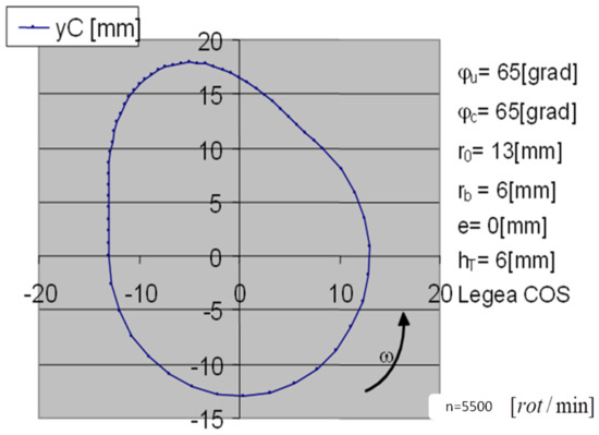
Figure 15.
Cam profile at module B. COSINE law, n = 5500 [rot/min] φu = 65 [degree], r0 = 13 [mm], rb = 6 [mm], hT = 6 [mm].
Figure 16 dynamically analyzes the C4P law, synthesized by the authors, starting from a speed n = 5500 [rot/min]. Negative acceleration peaks are very low (normal operation, with low noise and vibration). The effective (dynamic) lift of the valve is large enough, smax = 5.37 [mm], compared to h imposed by 6 [mm]. The yield is kept within normal limits, η = 8.3%. Figure 17 shows the corresponding profile.
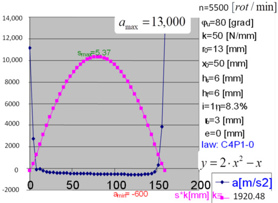
Figure 16.
Dynamic analysis at module B. C4P law, n = 5500 [rot/min] φu = 80 [degree], r0 = 13 [mm], rb = 3 [mm], hT = 6 [mm].
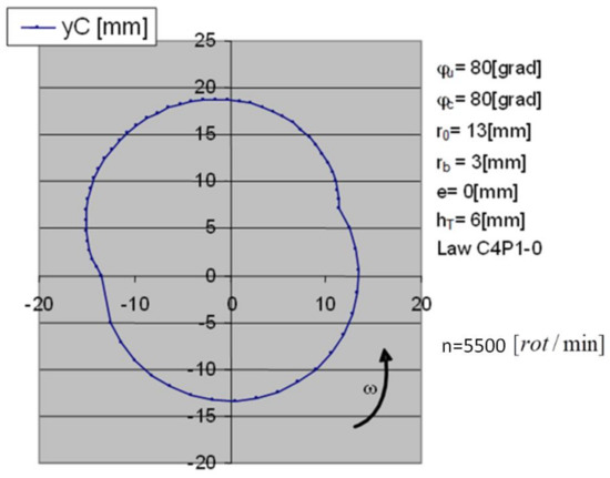
Figure 17.
Cam profile at module B. C4P law, n = 5500 [rot/min] φu = 80 [degree], r0 = 13 [mm], rb = 3 [mm], hT = 6 [mm].
4. Discussion
In this paper, the authors briefly present the basic dynamic aspects that appear in mechanisms with superior couples, used for hundreds of years in various machines and mechanisms, in mechanical transmissions, automations, automatic processing machines, industrial installations, medical equipment, control, and measurement in the automotive industry, in household appliances, and in many other fields. Today, robots frequently use such mechanical transmissions for servomotors.
Mechanisms with superior couples are extremely robust and reliable, withstand millions of dynamic cycles at high speeds and powers, transmit very high forces and moments for a long time, without breaks, without wear, and without repairs, while the mechanisms of Equivalent replacement tried so far may not cope with the breakage very quickly, for example, those with electrical coils and rod. For this reason, mechanisms with superior couples are also used in the medical industry in operating rooms, in the operation of industrial robots, in medical equipment, in control and measurement devices, in pacemakers, in mobile prostheses, and in other fields.
The laws of motion that have been used since ancient times in mechanisms with superior couples are now used in industrial robots, to obtain optimal laws for passers-by, for how to tread the sole of the robot as naturally as possible, but at the same time, such lifting laws also use the command and control of industrial robots, the trajectory of the deserter who must follow the correct laws of motion in the movement between two distant working points, to optimize the general movement of the robot and its arms, so the dynamics of movement must be smooth, but fast without noises, without vibrations, without interruptions, with higher speeds but constantly as high as possible, without unevenness, without breaks, without shocks, and without wear.
From ancient times, optimized polynomial laws have been used for this purpose: various, with as many factors as possible, to impose as many conditions at the border. Today there are other convenient laws that can be used in industrial robots, which are first synthesized by authors in hard memory mechanisms and then taken over and transposed for use in passing robots, as well as in all anthropomorphic industrial robots, which represent about 80–90% of all industrial robots, for optimizing their trajectories.
The authors started from the classic mechanisms with superior couples with cam and follower (adept; Figure 1), that worked with mechanical yields of about 3–4%, and gradually increased them to 10–12%, then to 18–24%, so that, in the end, they would even reach 30–40%, especially for roller modules [55,56,57,58,59,60,61,62,63].
Mechanisms with superior couple type Maltese cross or Geneva driver (Figure 2) have also been studied by the authors and it has been found that even they can increase mechanical efficiency even when using modern mechanisms inputs and many transverse channels that will no longer have only four channels, but many small ones, the guide on the channel being very short for the drive screw, so as to permanently change the drive screw and the driven channel, which leads to efficiencies over 90–95%.
Gears are also mechanisms with superior couples by multiplying the cams. The great advantage of the gear mechanism is to present permanent operating efficiencies, high power transmissions, forces, and moments, at high speeds, without wear, without shocks, and without noises or vibrations. Today, they are still very well calibrated constructively from the stage of design [58].
For the precise theoretical determination of the efficiency of a cylindrical gear, it must be taken into account that it will have several pairs of teeth engaged simultaneously, i.e., the degree of coverage of the gear must also be taken into account.
The efficiency of a toothed transmission is calculated, taking into account the fact that at a certain moment of gearing several pairs of teeth are in contact (in gearing), and not just one. The starting model was chosen as having four pairs of teeth engaged simultaneously. The first pair of teeth in the gear has the point of contact i, defined by the radius ri1, and the pressure angle αi1; the torque forces acting at this point are: the driving force Fmi, perpendicular to the position vector ri1 in i and the force transmitted from the driving wheel 1 to the driven wheel 2 through point i, Fτi, parallel to the gear line and having the direction from the wheel 1 to the wheel 2, the transmitted force being practically the projection of the driving force on the gear segment; the defined speeds are similar to the forces (considering the original, precise, described kinematics); the same parameters will be defined for the other three simultaneous contact points, j, k, l (Figure 18) [1,58].
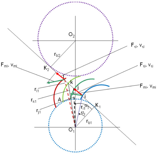
Figure 18.
Distribution of forces and speeds in a cylindrical gear when there are several pairs of teeth engaged simultaneously.
We do not intend in this paper to present the whole theory developed even if it is very interesting but only the final relations obtained (58)–(60).
The mechanical efficiency of a general gear will be obtained with the help of Equation (58), in which the degree of coverage, determined in advance with one of the Relation (59) or (60), will be introduced, depending on whether the gear is external or internal.
In Equation (58), the plus sign is taken as long as the driving wheel has external teeth and the minus sign will be given only when the driving wheel is a ring (crown) and has internal teeth.
5. Conclusions
Mechanisms with superior couples can, today, be optimally designed to work with high efficiency, for a long time, with no shocks, no vibrations, no noises, and no interruptions, and the role of this paper is to present some basic aspects of the dynamics of mechanisms with superior couples.
Since ancient times, gears have achieved high yields of 55–75%, so today we can design gears that achieve very high yields in operation between 85% and 99%.
And the Maltese cross-type mechanisms can be redesigned so that they work with very high yields of over 90% if, instead of an entrance, we project a lot of entrance bolts, and the cross channels will be built small and multiple, with dozens of channels that do not. They will remember the cross, and once the bolt enters a channel, it will work very shortly and will come out quickly, leaving another bolt to do the same with the next channel and so on.
The cam and adept mechanisms that traditionally worked with yields of 3–4% were designed by the authors to work with yields of 10–15% or 18–24%, but under certain conditions they can reach yields of 30–50%, a fact rarely encountered in such mechanisms.
For mechanisms with superior couples, the paper presents most of the essential aspects of dynamics, these being generally based on studies and older works of the authors, so there will only be presented some more important aspects simplified.
The importance of knowing the dynamics of the mechanisms with superior couples, so used in practice in robots, automation, automatic processing machines, medical equipment, and others, must not be highlighted again, with the justification being already reached in the presented paper.
The authors originally combined the Lagrange and Newton equations in order to obtain modern and intuitive dynamics with immediate applicability to the mechanisms with superior torques, cam-adept, and gears, but after the new dynamic methods introduced were already tested with other mechanisms such as with bars, motors, etc.
The distribution of forces was first introduced by the authors and it does not refer to the determination of forces acting on a mechanism. The reactions in the mechanism known from the classical methods determine the forces acting in the torques of the mechanism, and show the maximum loads in the mechanism as well as the variation of the inertia forces in the respective mechanism. The method of determining the distribution of forces shows the way in which the forces act in couples and on elements and especially the way in which they are transmitted from one element to another within the respective kinematic coupling. It is an original method that allowed in time the authors to deduce the exact mechanical efficiency of the mechanisms, the dynamic coefficients in the mechanism, the variation of the forces acting in the mechanism, and new methods for deducing the dynamics of the mechanism in question.
The exact dynamics of the mechanism is introduced with the support of the Lagrange equation of case I. The way in which the equation of motion of the car (Lagrange) is solved is completely original, and makes a great contribution to the study of machine dynamics. The method is presented for the classic distribution mechanism, where the cam is rotating, and the flat adept is in translational motion. The method can be adapted to any type of mechanism, plane, or spatial.
Author Contributions
We specify that both authors contributed equally to the entire realization of this work. All authors have read and agreed to the published version of the manuscript.
Funding
This research not yet received external funding.
Institutional Review Board Statement
Not applicable. Studies not involving humans or animals.
Conflicts of Interest
The authors declare no conflict of interest. The funders had no role in the design of the study; in the collection, analyses, or interpretation of data; in the writing of the manuscript, or in the decision to publish the results.
References
- Petrescu, F.I.T. Theoretical and Applied Contributions about the Dynamic of Planar Mechanisms with Superior Joints. Ph.D. Thesis, Polytechnic University of Bucharest, Bucharest, Romania, 2008. [Google Scholar] [CrossRef]
- Hren, I.; Hejma, P.; Michna, S.; Svoboda, M.; Soukup, J. Analysis of torque cam mechanism. MATEC Web Conf. 2018, 157, 06004. [Google Scholar] [CrossRef][Green Version]
- Zhao, H.F.; Zhang, Y.Q.; Zhang, S.Q. Production equipments and properties of low relaxation PC steel bar used for high railway ballastless track plates. Heat Treat. Met. 2010, 35, 101–103. [Google Scholar]
- Hiltcher, Y.; Guingand, M.; De Vaujauy, J.P. Numerical simulation and optimization of worm gear cutting. Mech. Mach. Theory 2006, 41, 1090–1110. [Google Scholar] [CrossRef]
- Zukovic, M.; Cveticanin, L.; Maretic, R. Dynamics of the cutting mechanism with flexible support and non-ideal forcing. Mech. Mach. Theory 2012, 8, 1–12. [Google Scholar] [CrossRef]
- Xueyan, H.; Kang, L.; Herong, J. Design of high precision online sizing cutter for PC Steel Bars. Adv. Mater. Res. 2013, 746, 520–523. [Google Scholar]
- Zheng, G.; Mao, S.M.; Li, X.E. Research on the theoretical tooth profile errors of gears machined by skiving. Mech. Mach. Theory 2016, 11, 1–11. [Google Scholar]
- Song, Y.M.; Tian, G.C.; Zhang, J. Prediction for dynamic characteristics of ring-plate planetary indexing cam mechanism. Mech. Mach. Theory 2001, 36, 143–152. [Google Scholar] [CrossRef]
- Tsai, C.Y. Mathematical model for design and analysis of power skiving tool for involute gear cutting. Mech. Mach. Theory 2016, 4, 195–208. [Google Scholar] [CrossRef]
- Zhang, J.F.; Zhang, J. A new dynamics modeling and simulation for eccentric cam mechanism. China Mech. Eng. 2010, 21, 535–539. [Google Scholar]
- Gao, J.H. Study on the sinusoid and polynomial curve. J. Mech. Transm. 2010, 34, 31–35. [Google Scholar]
- Yan, H.S.; Tsai, M.C. An experimental study of the effects of cam speeds on cam-follower systems. Mech. Mach. Theory 1996, 31, 397–412. [Google Scholar] [CrossRef]
- Gatti, G.; Mundo, D. On the direct control of follower vibrations in cam–follower mechanisms. Mech. Mach. Theory 2010, 45, 23–35. [Google Scholar] [CrossRef]
- Hamza, F.; Abderazek, H.; Lakhdar, S.; Ferhat, D.; Yıldız, A.R. Optimum design of cam-roller follower mechanism using a new evolutionary algorithm. Int. J. Adv. Manuf. Technol. 2018, 99, 1267–1282. [Google Scholar] [CrossRef]
- Hirschhorn, J. Pressure angle and minimum base radius. Mach. Des. 1962, 34, 191–192. [Google Scholar]
- Fenton, R.G. Determining minimum cam size. Mach. Des. 1966, 38, 155–158. [Google Scholar]
- Terauchi, Y.; El-Shakery, S.A. A computer-aided method for optimum design of plate cam size avoiding undercutting and separation phenomena. Mech. Mach. Theory 1983, 18, 157–163. [Google Scholar] [CrossRef]
- Bouzakis, K.D.; Mitsi, S.; Tsiafis, I. Computer aided optimum design and NC milling of planar cam mechanisms. Int. J. Mach. Tool Manuf. 1997, 37, 1131–1142. [Google Scholar] [CrossRef]
- Lampinen, J. Cam shape optimization by genetic algorithm. Comput. Aided Des. 2003, 35, 727–737. [Google Scholar] [CrossRef]
- Carra, S.; Garziera, R.; Pellegrini, M. Synthesis of cams with negative radius follower and evaluation of the pressure angle. Mech. Mach. Theory 2004, 39, 1017–1032. [Google Scholar] [CrossRef]
- Tsiafis, I.; Paraskevopoulou, R.; Bouzakis, K.D. Selection of optimal design parameters for a cam mechanism using multi-objective genetic algorithm. Ann. Constantin Brancusi Univ. TarguJiu Rom. Eng. Ser. 2009, 2, 57–66. [Google Scholar]
- Shigley, J.E. Theory of Machines and Mechanisms, 1st ed.; Oxford University Press: New York, NY, USA, 2011. [Google Scholar]
- Angeles, J.; Cajún, L.; Carlos, S. Optimization of Cam Mechanisms, 1st ed.; Springer: Cham, The Netherlands, 2012. [Google Scholar]
- Flores, P. A computational approach for cam size optimization of disc cam follower mechanisms with translating roller followers. J. Mech. Robot. 2013, 5, 041010. [Google Scholar] [CrossRef]
- Hidalgo-Martinez, M.; Sanmiguel-Rojas, E.; Burgos, M.A. Design of cams with negative radius follower using Bézier curves. Mech. Mach. Theory 2014, 82, 87–96. [Google Scholar] [CrossRef]
- Gheadnia, H.; Cermik, O.; Marghitu, D.B. Experimental and theoretical analysis of the elasto-plastic oblique impact of a rod with a flat. Int. J. Impact Eng. 2015, 86, 307–317. [Google Scholar] [CrossRef]
- Yi, W.; Li, X.; Gao, L.; Zhou, Y.; Huang, J. ε constrained differential evolution with pre-estimated comparison using gradient-based approximation for constrained optimization problems. Expert Syst. Appl. 2016, 44, 37–49. [Google Scholar] [CrossRef]
- Hsu, K.L.; Hsieh, H.A. Positive-drive cam mechanisms with a translating follower having dual concave faces. J. Mech. Robot. 2016, 8, 044504. [Google Scholar] [CrossRef]
- Jana, R.K.; Bhattacharjee, P. A multi-objective genetic algorithm for design optimisation of simple and double harmonic motion cams. Int. J. Des. Eng. 2017, 7, 77–91. [Google Scholar] [CrossRef]
- Hammoudi, A.; Djeddou, F.; Atanasovska, I. Adaptive mixed differential evolution algorithm for bi-objective tooth profile spur gear optimization. Int. J. Adv. Manuf. Technol. 2017, 90, 2063–2073. [Google Scholar]
- Halicioglu, R.; Dulger, L.C.; Bozdana, A.T. Modeling, design, and implementation of a servo press for metal-forming application. Int. J. Adv. Manuf. Technol. 2017, 91, 2689–2700. [Google Scholar] [CrossRef]
- Thompson, J.M.; Thompson, M.K. ANSYS Mechanical APDL for Finite Element Analysis, 1st ed.; Butterworth-Heinemann: Oxford, UK, 2017. [Google Scholar]
- Yu, C.; Meng, X.; Xie, Y. Numerical simulation of the effects of coating on thermal elastohydrodynamic lubrication in cam/tappet contact. Proc. Inst. Mech. Eng. J Eng. Tribol. 2017, 231, 221–239. [Google Scholar] [CrossRef]
- Torabi, A.; Akbarzadeh, S.; Salimpour, M. Comparison of tribological performance of roller follower and flat follower under mixed elastohydrodynamic lubrication regime. Proc. Inst. Mech. Eng. J Eng. Tribol. 2017, 231, 986–996. [Google Scholar] [CrossRef]
- Qin, W.; Zhang, Z. Simulation of the mild wear of cams in valve trains under mixed lubrication. Proc. Inst. Mech. Eng. J Eng. Tribol. 2017, 231, 552–560. [Google Scholar] [CrossRef]
- Yousuf, L.S.; Marghitu, D.B. Non-linear dynamic analysis of a cam with flat-faced follower linkage mechanism. In Proceedings of the ASME 2017 International Mechanical Engineering Congress and Exposition, IMECE 2017, Tampa, FL, USA, 3–9 November 2017. [Google Scholar]
- Fei, G.; Liu, Y.; Liao, W.H. Cam profile generation for cam-spring mechanism with desired torque. J. Mech. Robot. 2018, 10, 041009. [Google Scholar]
- Umar, M.; Mufti, R.A.; Khurram, M. Effect of flash temperature on engine valve train friction. Tribol. Int. 2018, 118, 170–179. [Google Scholar] [CrossRef]
- Alakhramsing, S.S.; de Rooij, M.B.; Schipper, D.J.; Drogen, M.V. Lubrication and frictional analysis of cam–roller follower mechanisms. Proc. Inst. Mech. Eng. J Eng. Tribol. 2018, 232, 347–363. [Google Scholar] [CrossRef]
- Halicioglu, R.; Dulger, L.C.; Bozdana, A.T. Improvement of metal forming quality by motion design. Robot. Comput.-Integr. Manuf. 2018, 51, 112–120. [Google Scholar] [CrossRef]
- Al-Hamood, A.; Jamali, H.U.; Abdullah, O.I.; Senatore, A.; Kaleli, H. Numerical analysis of cam and follower based on the interactive design approach. Int. J. Interact. Des. Manuf. 2019, 13, 841–849. [Google Scholar] [CrossRef]
- Alakhramsing, S.S.; de Rooij, M.; Akchurin, A.; Schipper, D.J.; van Drogen, M. A mixed-TEHL analysis of cam-roller contacts considering roller slip: On the influence of roller-pin contact friction. J. Tribol. 2019, 141, 011503. [Google Scholar] [CrossRef]
- Ciulli, E.; Pugliese, G.; Fazzolari, F. Film thickness and shape evaluation in a cam-follower line contact with digital image processing. Lubricants 2019, 7, 29. [Google Scholar] [CrossRef]
- Jamali, H.U.; Al-Hamood, A.; Abdullah, O.I.; Senatore, A.; Schlattmann, J. Lubrication analyses of cam and flat-faced follower. Lubricants 2019, 7, 31. [Google Scholar] [CrossRef]
- Pugliese, G.; Ciulli, E.; Fazzolari, F. Experimental aspects of a cam-follower contact. In Advances in Mechanism and Machine Science; Uhl, T., Ed.; Springer: Cham, Switzerland, 2019; Volume 73, pp. 3815–3824. [Google Scholar]
- Yousuf, L.S.; Hadi, N.H. Contact Stress Distribution of a Pear Cam Profile with Roller Follower Mechanism. Chin. J. Mech. Eng. 2021, 34, 24. [Google Scholar] [CrossRef]
- Yang, T.H.; Jo, G.; Koo, J.H.; Woo, S.Y.; Kim, J.U.; Kim, Y.M. A compact pulsatile simulator based on cam-follower mechanism for generating radial pulse waveforms. Biomed. Eng. Online 2019, 18, 1. [Google Scholar] [CrossRef]
- Li, C.; Xiong, H.; Pirbhulal, S.; Wu, D.; Li, Z.; Huang, W.; Zhang, H.; Wu, W. Heart-carotid pulse wave velocity a useful index of atherosclerosis in Chinese hypertensive patients. Medicine 2015, 94, e2343. [Google Scholar] [CrossRef]
- Nelson, M.R.; Stepanek, J.; Cevette, M.; Covalciuc, M.; Hurst, R.T.; Tajik, A.J. Noninvasive measurement of central vascular pressures with arterial tonometry: Clinical revival of the pulse pressure waveform? Mayo Clin. Proc. 2010, 85, 460–472. [Google Scholar] [CrossRef] [PubMed]
- Katsuhiko, K.; Yasuharu, T.; Akira, O.; Yoshinori, M.; Tatsuya, K.; Tetsuro, M. Radial augmentation index: A useful and easily obtainable parameter for vascular aging. Am. J. Hypertens. 2005, 18, 11S–14S. [Google Scholar]
- Kuniharu, T.; Toshitake, T.; Johnny, C.H.; Hyunhyub, K.; Andrew, G.G.; Paul, W.L.; Ronald, S.F.; Ali, J. Nanowire active-matrix circuitry for low-voltage macroscale artificial skin. Nat. Mater. 2010, 9, 821–826. [Google Scholar] [CrossRef]
- Turner, M.; Speechly, C.; Bignell, N. Sphygmomanometer calibration—Why, how and how often? Aust. Fam. Phys. 2007, 36, 834–837. [Google Scholar]
- Bae, J.H.; Ku, B.; Jeon, Y.J.; Kim, H.; Kim, J.; Lee, H.; Kim, J.Y.; Kim, J.U. Radial pulse and electrocardiography modulation by mild thermal stresses applied to feet: An exploratory study with randomized, crossover design. Chin. J. Integrat. Med. 2017. [Google Scholar] [CrossRef] [PubMed]
- Kim, Y.M. Precise measurement method of radial artery pulse waveform using robotic applanation tonometry sensor. J. Sens. Sci. Technol. 2017, 26, 135–140. [Google Scholar] [CrossRef]
- Petrescu, F.I.; Petrescu, R.V. Otto Motor Dynamics. Rev. Geintec-Gestao Inov. Tecnol. 2016, 6, 3392–3406. [Google Scholar]
- Petrescu, F.I.T.; Petrescu, R.V. Dynamics of the Distribution Mechanism with Rocking Tappet with Roll. Indep. J. Manag. Prod. 2019, 10, 951–965. [Google Scholar] [CrossRef]
- Petrescu, F.I.T.; Petrescu, R.V.; Mirsayar, M.M. The Computer Algorithm for Machine Equations of Classical Distribution. J. Eng. Struct. 2017, 4, 193–209. [Google Scholar]
- Petrescu, F.I.T.; Petrescu, R.V. High-Efficiency Gears. Facta Univ.-Ser. Mech. Eng. 2014, 12, 51–60. [Google Scholar]
- Petrescu, F.I.; Petrescu, R.V. Machine Equations to the Classical Distribution. Int. Rev. Mech. Eng. 2014, 8, 309–316. [Google Scholar]
- Petrescu, F.I.; Petrescu, R.V. An Algorithm for Setting the Dynamic Parameters of the Classic Distribution Mechanism. Int. Rev. Modell. Simul. 2013, 6, 1637–1641. [Google Scholar]
- Petrescu, F.I.; Petrescu, R.V. Forces and Efficiency of Cams. Int. Rev. Mech. Eng. 2013, 7, 507–511. [Google Scholar]
- Petrescu, F.I.T. Geometrical Synthesis of the Distribution Mechanisms. Am. J. Eng. Appl. Sci. 2015, 8, 63–81. [Google Scholar] [CrossRef]
- Petrescu, R.V.; Aversa, R.; Apicella, A.; Petrescu, F.I. Future Medicine Services Robotics. Am. J. Eng. Appl. Sci. 2016, 9, 1062–1087. [Google Scholar] [CrossRef]


Publisher’s Note: MDPI stays neutral with regard to jurisdictional claims in published maps and institutional affiliations. |
© 2021 by the authors. Licensee MDPI, Basel, Switzerland. This article is an open access article distributed under the terms and conditions of the Creative Commons Attribution (CC BY) license (https://creativecommons.org/licenses/by/4.0/).