1. Introduction
The signification of Cement and Concrete Composites (CCC) can vary and often have a broad meaning in the scientific field. European standard EN 197-1 [
1] lists 27 common types of cement, divided into five groups (ordinary Portland cement and cement mixes) with a notation that those are hydraulic binders [
2]. Furthermore, the ASTM C 125 [
3] standard acknowledges concrete that primarily employs hydraulic cement as a binding medium but does not entirely exclude the existence of non-hydraulic binders [
4]. From a scientific point of view, materials such as aluminosilicates and calcium silicates are also recognised as cementitious materials, even though they do not imply hydration as the main hardening process. The former is a powdered substance, also called alkali-activated cement or geopolymer [
5,
6], whereas the latter hardens through a carbonation process [
7]. Because of the above, concrete, mortar and grout are composite materials that can contain either hydraulic or non-hydraulic binder. In this research paper, the term concrete composite is associated with any concrete mix (containing fibres or other types of reinforcement, special aggregates and polymers) that can be viewed as ageing viscoelastic materials [
8,
9,
10].
Viscoelastic behaviour (creep and relaxation) of CCC is considered when evaluating material suitability for practical use, as are the restrained and unrestrained shrinkage properties. Estimation of such effects must be integrated into the design process [
11,
12,
13]. Thus, long-term properties of CCC have been widely studied over the years, especially to acquire applicable knowledge about world-known and novel structural materials [
14,
15,
16,
17,
18].
In terms of CCC mechanical properties, mainly qualities such as compressive strength and behaviour under sustained compressive loading have been researched and appreciated. Conventionally, in the design process of reinforced concrete, the CCC capacity of withstanding tensile stresses is neglected [
19,
20]. However, crack propagation under tensile loading is one of the main types of CCC failure mechanisms at the service limit state (along with crushing under compression at ultimate limit state), and even uniaxial compression failure can be considered as being due to tensile stresses [
8,
21]. Fibre reinforcement is proven to increase ductility, tensile and flexural resistance, as well as to diminish shrinkage at an early age and crack propagation [
19,
22,
23,
24]. To date, scientific progress has led to interests in various subfields of fracture mechanics and tensile bearing capacity with respect to diverse loading rates [
21,
25,
26,
27]. CCC tensile properties are investigated mainly by performing indirect tensile tests, where specific characteristic values can be derived. Direct uniaxial tensile tests are less common since it is problematic to maintain a test specimen within a loading rig under sustained uniform tensile stress [
14,
20,
25,
28,
29]. Assessing the tensile strength of CCCs depends on the testing method used. The indirect tensile strength test provides higher strength than the direct uniaxial tensile tests, but the latter is considered more accurate [
30,
31]. Nevertheless, there is no standardised method for performing such a test [
31].
RILEM TC232-TDT [
32] recommends using parallelepiped shape specimens (with minimum dimensions of 500 × 60 × 6 mm) for testing textile-reinforced concrete in uniaxial tension. The document recommends the use of LVDTs but also refers to ISO 9513 [
33] regarding the required accuracy of extensometers. According to ISO 9513:2012 [
33], extensometers can be either contacting or non-contacting (e.g., laser, DIC).
Digital image correlation (DIC) is a non-contact, optically based research technique that allows the monitoring of various derived quantities-of-interest (QOIs) at the surface of a test specimen. Through this method, point displacements, strains, surface curvature and velocities can be tracked. For such analysis, one (for 2D-DIC) or two (for 3D-DIC) digital cameras are used instead of conventional surface-attached measuring devices (e.g., linear variable displacement transformers or LVDTs, foil strain gauges, dial indicators, etc.). During the mechanical test, a specimen can be continuously monitored by recording a video or capturing images. Afterwards, the acquired images are processed by DIC software that evaluates the desired QOIs by analysing both point displacements and deviations from the initial state. The 2D-DIC technique is effective when the object is planar to the camera sensor and not moving with respect to the camera [
34], whereas the 3D-DIC system (also known as stereo-DIC) tolerates relative movements and allows one to complete the calculations properly even with convex/concave-shaped specimens [
35].
Cost-effectiveness is one of the reasons that researchers increasingly more often prefer non-contact measuring techniques over conventional systems. Since 2D-DIC is a monocular system and requires a single camera (with a stand, positioning mechanism and lighting kit), the expenses are significantly lower than for the 3D-DIC setup that requires at least double the amount of investment. Furthermore, computer software for 2D-DIC is normally less expensive (or even free of charge) and easier to operate. As 3D-DIC is beyond the scope of this research work, it will not be discussed in further detail. Various scientists have validated optical-based research techniques by using scientific-grade digital cameras. Such selection of equipment is also advised by the International Digital Image Correlation Society [
34]. However, there have been successful studies that prove relatively inexpensive digital single-lens reflex (DSLR) cameras to be appropriate as well [
36,
37].
In practical use, the DIC technique can significantly ease surveys of CCC structures such as bridges, tunnel linings, containment vessels of nuclear reactors and others, that can be described as inaccessible to humans, hazardous environments or excessively large in the surface area [
38,
39]. Another advantage of DIC is the ability to analyse QOIs at any position and direction within the field of view (FOV). Therefore, unlike with surface-attached measuring devices, with image correlation software, various changes can be evaluated that could not be predicted before the test (e.g., strain and crack propagation at unsuspected locations or amplitude) [
34,
40]. Furthermore, in some cases, deformations can exceed the limitations of the attachable extensometer gauge lengths and fastening accessories, leading to faulty data, an absence of data or even ending the test [
37]. In general, the versatility of the DIC method allows it to be applied for both direct and indirect mechanical tensile testing.
In this research work, 2D-DIC was employed to monitor fibre-reinforced Portland cement composite tensile creep deformation. Compact Tension (CT) specimens were monitored under sustained uniaxially applied tensile load over 50 days. Similar specimen geometry is suggested by ISO 7539 [
41], ASTM E647 [
42] and ASTM E399 [
43] standards. Such specimen geometry allows to investigate both elastic and plastic deformations as well as fracture mechanics. An entry/mid-level DSLR camera was used to capture the images, whereas the analysis was done using the GOM Correlate free software. In addition, the acquired data were compared with conventional surface-attached strain gauges measurements. Such long-term DIC experiments have not been previously done.
2. Materials and Methods
2.1. Composite Mix
For testing purposes, an OPC composite with 1 wt% (PVA) fibres was prepared. Detailed mix properties are given in
Table 1. The composite was mixed and moulded into standard 150 × 150 × 150 mm oiled steel moulds. After curing for 24 h (in +20 °C, wet conditions), the cubes were demoulded and submerged in water for seven days for hardening. Standard ageing conditions (temperature 20 ± 2 °C, RH > 95 ± 5%) were provided during hardening.
As shown in the mix properties, the obtained composite is characterised by a cement-to-sand ratio of 1:2. PVA fibres were added to increase crack resistance, ductility and reduce shrinkage at anearly age of OPC concrete.
2.2. Preparation of CT Specimens
The selected specimen shape resembles the one used for the evaluation of crack propagation in metals (ASTME647 [
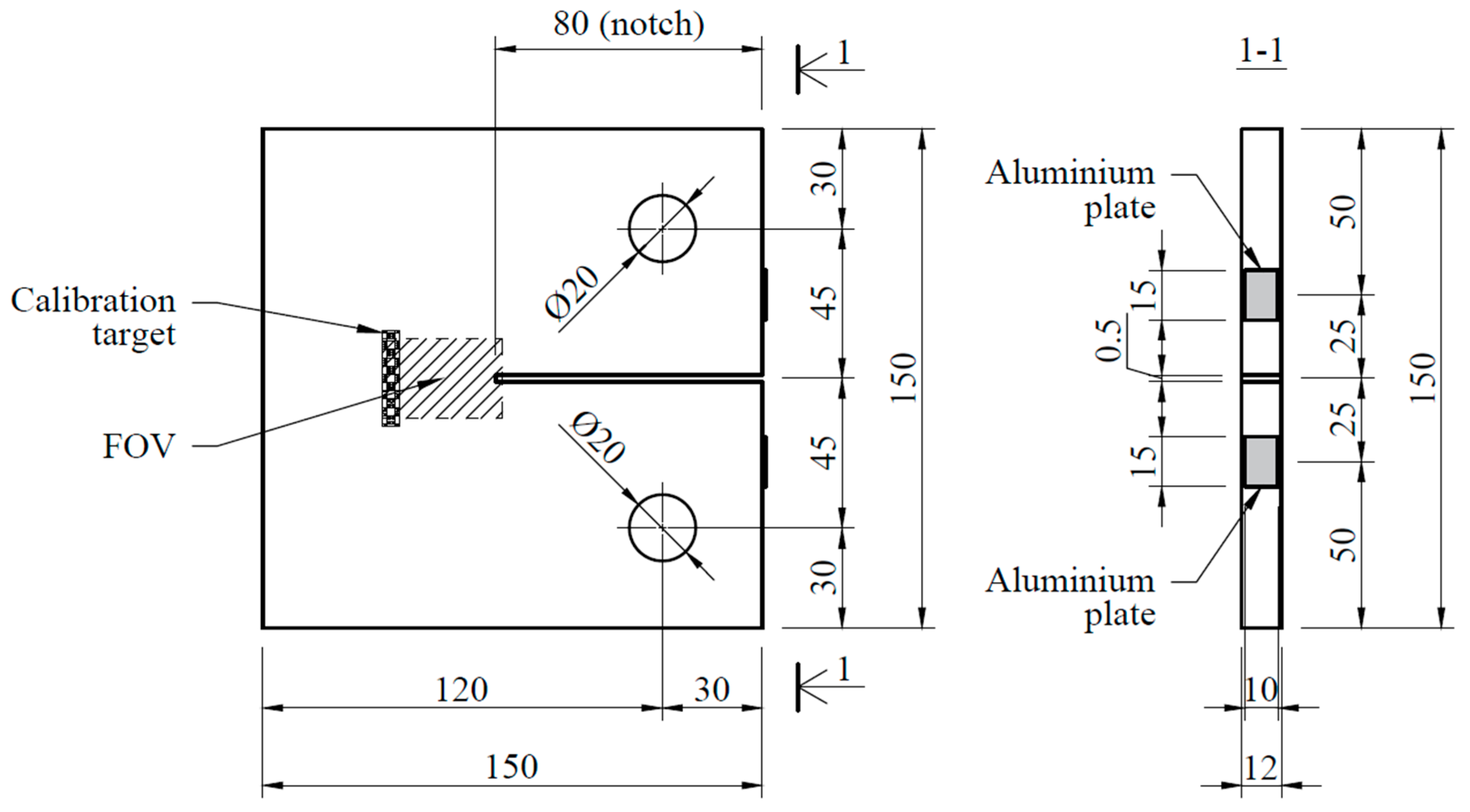
42]), the so-called Compact Tension (CT) specimen. Preparation of CT specimens was done after 7 days of curing. The cured composite cubes were saw-cut into 12 mm thick plates, using a stationary block cutter with a diamond saw blade. In cases of uneven cutting plane, the surface was manually smoothened with an angle grinder (with a diamond grinding disk). Clear access to the surface where the tensile creep strain progression becomes visible was important. To predict the maximum stress intensity zone and limit the FOV area (where the creep strains initiate), the 80 mm long and 0.5 mm wide notch was cut using a tabletop bandsaw Proxxon Micromot MBS 240/E (with a diamond blade). The tensile stress maximum intensity was achieved at the tip of the notch. The depth of the specimen was also reduced, promoting the plane stress state. The available path for the progress of the initiated strain parallel to the notch was 30 mm. The distance between the loading axis and the tip of the notch was 50 mm. Two drill holes with a diameter of 20 mm were made in further steps, where a stationary drilling machine (with a diamond drilling crown) was used. Summarising, the dimensions adopted for the specimens were 150 mm by 150 mm (perpendicular and parallel to the notch) and 12 mm (thickness). CT specimen geometry was prepared according to
Figure 1. The preparation of such a methodology provides test specimens representing the situation close to real CCC structures since the fibres are oriented randomly and dispersed relatively evenly throughout the volume.
When the specimens were finished, they were thoroughly cleaned under running tap water and dried in room condition (+20 °C, RH = 60%) for 24 h. After that, the region of FOV of each specimen was observed, and any protruding parts of the fibres were trimmed by hand using a thin razor blade. Trimming has a beneficial effect on further surface preparation. Such an action was also taken due to the previous trialling where unwanted shadows from sticking fibre ends were noticed (in the DIC images). In some cases, even such diminutive surface irregularities can complicate camera focusing (discussed in
Section 2.3).
2D-DIC is based on such a principle that a unique surface pattern follows the deformed object itself while a mechanical test is performed. Then, several digital images are taken that capture changes throughout the time. Preferably, DIC software uses a dense stochastic speckle pattern at the surface of the test specimen to create overlapping subsets of points, matching and analysing deviations from the initial state (e.g., the first image in the series, also called the reference image) [
34]. For applying a speckle pattern, an airbrush Royalmax TC-12K with black acrylic-based spray paint was used. In earlier trials, it was found that the speckle pattern tends to emanate and fade due to absorbing into the uncoated, porous surface of the material. Furthermore, in this research, white Aalborg cement was used for the mortar mix; thus, a bright white colour tone (close to RAL 9016) was obtained for the final hardened material. Because of such properties of the surface, the captured images happened to be overexposed (there was no valid solution found by adjusting the camera or the lighting settings). The DIC software could not evaluate the strains at the desired locations within the FOV. Considering previously mentioned obstacles, the surface of each test specimen was first coated with two layers of light grey (RAL 7047), nonglossy watercolour (applied with a brush). After 24 h of drying, black paint speckles were sprayed onto the coated surface region. Similar preparation technology has been used by L.Graziani et al. [
44].
In the DIC software, real displacement values are calculated to user-defined reference intervals. Therefore, in this research, a surface-attached calibration target was glued to the specimen’s surface and used within the FOV. The target with a 2.5 × 2.5 mm checkerboard pattern was laser-printed on a self-adhesive plastic sheet (similar to standard copy paper −0.1 mm in thickness). Ordinary office printing technology (laser-printing on non-coated paper) was shown to be less effective due to the limited sharpness of the printed borderlines between black and white regions.
Before experimental tests, two aluminium plates 15 × 10 × 0.8 mm were glued to the side of each specimen (using 2-part epoxy resin). After that, one digital dial gauge with ±0.001 mm resolution was centrally and symmetrically positioned at the edge of each specimen. Strain gauges were placed so that their attachment points were located on the glued aluminium plates; the strain gauge length was 50 mm. Strain gauges were attached to the specimens with elastic rubber bands (
Figure 2).
Then, each specimen was fixed into a lever arm creep rig and loaded. All creep specimens were loaded with a constant, static, tensile load and strain readings were regularly performed. In this case, for CT specimens, notch mouth opening displacement (NMOD) was monitored. Parallel to NMOD readings, the notch tip zone was captured daily with a digital camera (for further notch tip opening displacement—NTOD analysis). For detailed information about taking NTOD readings, please see
Section 2.3.
On the first day of the long-term test, the strain readings were done before loading and after all the calculated load had been applied. For the first 6 to 8 h, the readings were taken at hourly intervals. The next two-week readings were recorded at daily intervals. Then the following week, readings were taken at 2–3-day intervals. Similarly, to determine the correct creep behaviour, similarly shaped shrinkage specimens were placed in identical environmental conditions and their strain was monitored (no load applied to the shrinkage specimens). Conclusions were made based on subtracting the shrinkage strain values from the tensile creep values. The basic and drying creep components have not been determined separately.
2.3. Creep Test, DIC Application
The CT testing procedures developed for the present work consisted of applying a tensile load to a single-edge notched specimen. Before the creep test, the ultimate tensile load was determined for the CT specimens. A universal testing machine with an accuracy of ±0.5% for destructive ultimate load tests was used (rate of loading 0.3 mm/min). For creep tests, mechanical lever arm creep rigs were used. With these rigs, it is possible to apply constant loading to the specimens and to keep it uniform over a long period. Furthermore, it is not necessary to adjust the stress level during the experiments. The calibration curves are linear; no external energy resources are used. The lever arm ratio of the lever arm creep rig was 1:20. The loading level was adjusted to an accuracy of ±2% (determined by an analogue dynamometer with 0.002 kN resolution). The geometry of the test specimens was kept the same for all tests.
A single CT specimen was placed vertically in a creep rig, ensuring alignment with the loading axis. Each specimen was fixed (within the creep rig), using two grips (connected with bolts through the ⌀20 mm drill holes) that transmit the applied tensile loading (
Figure 2b). The fastening system was made so that the upper and lower attachment points are hinged (pinned) supports; hence, the specimen is free to rotate, and no additional stresses are caused due to eccentric loading. A more detailed description of the exact creep apparatus (inventory of Riga Technical University) can be found in [
45]. Specimens were kept under constant load levels corresponding to 60% of the ultimate tensile load. A tensile dynamometer ДПУ-0.02-2 (resolution 0.002 kN, measuring range 0–0.2 kN) was enclosed within the loading rig to monitor precise levels of applied force. The load was applied gradually in five steps and as fast as possible. The modulus of elasticity was determined from the elastic strains that occurred at the beginning of the creep test. According to Hooke’s law, the modulus of elasticity was determined by measuring the elastic strain on each loading step. After that, the specimens were kept under a constant load for 50 days. The long-term test was performed in a dry atmosphere of controlled relative humidity in standard conditions t = 20 ± 3 °C, RH = 50 ± 5%.
Complete creep testing and DIC imaging setup are shown in
Figure 2. DIC imaging setup: (
a) Camera facing the loaded test specimen, camera controlled via digiCamControl free software (FOV visible in the PC display); (
b) camera tripod with stabilising weight, positioning mechanism, DSLR with macro ring flash, CT specimen with an attached strain gauge.
Previously, a similar DIC imaging setup was successfully used by M.Francic Smrkic et al. [
37]. In this research work, the propagation of the tensile strain was traced on the surface of the specimens using a digital camera, Canon EOS550D DSLR (APS-C sensor) with the Canon EF-S 60 mm F/2.8 macro lens. The optimal distance between the camera sensor and the specimen was found to be 235 mm, thus FOV was 36 × 24 mm. For optimal light conditions, a Meike MK-14EXT Macro Ring flash was attached to the lens. Due to insufficient sturdiness, extra rubber bands within the connecting junction and self-adhesive tape around the attachment ring were placed to hold the flash in a constant position (otherwise resulting in changing exposure). No additional external/ambient light sources were put to use.
The camera was placed on a tripod Manfrotto MT055XPRO3 (aluminium). For extra vibration resistance, a 2.1 kg weight was hung in the tripod’s central node. For operational convenience, the camera fastening system (upon the tripod) was combined from several parts (listed upwards according to the placement on the tripod): Levelling head Puluz (with three adjustment screws), panorama head Rolley Pan Head R60, micropositioning rail Puluz, discal clamp FittestPhoto YP-65, quick release plate FittestPhoto PU-70 (for attaching to the camera). Such a setup allows to move and rotate the camera gradually relative to the test specimen.
Before loading, the camera was connected to a PC and trial images were captured via digiCamControl free software; the optimal camera settings were manually adjusted as follows: Aperture F/16, exposure time 1/25 s, ISO speed ISO-100, flash speed 1/64 s (no exposure compensation). Captured images were 5184 × 3456 px in size. Additionally, acquired images were checked with GOM Correlate software to evaluate pattern quality.
Since in 2D-DIC, it is crucial to prevent any camera movements from the initial position, all DIC images during the test were captured remotely using a wired shutter release device Jintu RS-60E3. DIC images were captured starting immediately after load application (in the loading rig) (according to the time intervals as mentioned in
Section 2.2). Concurrently, displacement data were manually registered using an electrical dial gauge IP54 (resolution 0.001 mm, measuring range 0–10 mm) attached to the notched side of the CT specimen.
The acquired digital images were imported and processed in GOM Correlate free software—scaled in respect to the calibration target and analysed. The first image of the series (captured immediately after loading) was selected as the reference stage. To compare data from the DIC analysis to the electrical dial gauge, virtual extensometers were created in the software, from which data were exported for further analysis (image processing was done in accordance with [
40]).
3. Results and Discussion
Figure 3 represents the stress/displacement distribution throughout the FOV area. There were three virtual extensometers (gauge length—10 mm) placed in different areas of the FOV—close to the notch tip, central of the FOV and at the left edge of the FOV (along with the calibration target) (
Figure 3) An additional virtual extensometer (gauge length—10 mm) was placed 1 mm into the notch area (beyond the FOV). The analysis was done using DIC software.
The virtual extensometers used in the stress analysis were set to monitor distance changes relative to the reference stage (first image captured during the test). The graph reveals that the zones further from the notch tip are more prone to displacement than those that are placed closer and previously believed to bear higher strains. This subject is to be studied in more detail in further research.
In this experiment, the area of the CT specimen’s notch tip was captured on a DSLR camera to compare the displacement data from the DIC with those registered by surface-attached dial gauges. Five virtual extensometers (gauge length—2 mm) were created in GOM software for the DIC analysis. The extensometers were placed within the notched zone of the specimen (0.5 mm into the notch towards the open end), positioned perpendicular to the notch (
Figure 4). Such a location of the extensometers was chosen to enable displacement analysis (by DIC software) that can be verified with mathematical calculations (manually). Data represented by GOM software were exported to MS Excel for further analysis.
In further analysis, all displacement data obtained from the DIC were compared with displacement data from surface-attached strain gauges.
Figure 5 shows the test specimen with the measuring device and the data obtained.
Displacement data from surface attached digital dial gauge (NMOD) show similarities to data from the DIC analysis (NTOD) (
Figure 6). Both curves are similar in their overall nature and tend to break simultaneously when showing reactions of the material (e.g., day 15 and day 24).
For further analysis of data compatibility, the mechanically measured displacements in the NMOD zone were used to mathematically calculate the corresponding NTOD values by similar triangles principle. The obtained results are shown in
Figure 7.
DIC analysis in GOM Correlate software shows a larger NTOD displacement compared to those calculated from the dial gauge data. The trend of both curves is similar.
Additionally, calculation principles by Saxena (1978) [
46] were used to calculate the displacements along the loading axis (
Figure 8).
The following Equations (1)–(4) were used to calculate the displacements along the loading axis (
) [
46].
Opening at the crack edge:
Configuration functions for displacement:
where
is the concentrated load and
is the elastic constant.
Equations (1)–(3) were applied so that
represents NMOD and
represents the displacement along loadline. Displacement values that were obtained from physical measurements, DIC analysis and mathematical calculations are shown in
Figure 9.
As the calculations of displacement along the load line are dependent on the physically obtained displacement data, all displacement curves show close similarities in shape, whereas the absolute displacement values differ significantly. Such differences are reasoned by the unique geometry of a CT specimen—the deformation dynamic (under the designated load) at the free end of the notch is more rapid than the zone closer to the notch tip.


 ,
, 


